HAL Id: hal-00505544
https://hal.archives-ouvertes.fr/hal-00505544
Submitted on 24 Jul 2010
HAL is a multi-disciplinary open access
archive for the deposit and dissemination of
sci-entific research documents, whether they are
pub-lished or not. The documents may come from
teaching and research institutions in France or
abroad, or from public or private research centers.
L’archive ouverte pluridisciplinaire HAL, est
destinée au dépôt et à la diffusion de documents
scientifiques de niveau recherche, publiés ou non,
émanant des établissements d’enseignement et de
recherche français ou étrangers, des laboratoires
publics ou privés.
Arc root interaction with the electrode: a comparative
study of 1D-2D axi symmetric simulations
M’Hammed Abbaoui, A. Lefort
To cite this version:
M’Hammed Abbaoui, A. Lefort. Arc root interaction with the electrode: a comparative study of
1D-2D axi symmetric simulations. European Physical Journal: Applied Physics, EDP Sciences, 2009,
48 (1), pp.1-9. �10.1051/epjap/2009134�. �hal-00505544�
(will be inserted by the editor)
Arc Root Interaction with the Electrode: a Comparative Study
of 1D-2D Axi Symmetric Simulations
M. ABBAOUI and A. LEFORT
LAEPT - Clermont University-CNRS, Blaise Pascal University, Physique 5, 24 avenue des Landais, F63177 AUBIERE Cedex Received: date / Revised version: date
Abstract. Two simulation methods of the energy transmitted by the arc roots to the electrode material are described and their results are compared together and with these found by other authors. About a copper electrode the time phase evolutions are given when a constant energy flux is applied to the contact surface. The obtained results are better for vacuum and small current. The cathode and anode result discussions lead to propositions to improve arc root models.
PACS. PACS-key 52.40.Hf – PACS-key Plasma-material interactions; boundary layers effects
1 Introduction
The existence of electric arc discharge needs transition zones between the thermal plasma and the metallic elec-trodes, the emission of electrons (cathode) and their cap-ture (anode) is not possible without energy exchange and its consequences: the electrode surface transformations. It is necessary to understand the material transformations and to use them in the best conditions; the goal is not the same in welding or in breaker contacts. At the cathode arc root, the emitting centres are disconnected in arc vacuum and adjacent in others cases, they are called fragments, the present study is relative to one fragment cathode. The
an-ode arc root exists only to collect column electrons that transmit their energy to the electrode, as in the fragments they have a circular shape. To study material evolution two simulation methods are used:
- the 1D simulation represents a first approach and gives the first results necessary to justify the validity of our work,
- the 2D axi symmetric simulation is firstly technically verified by comparison with 1D results.
The choice of a two presentation methods is to show the importance (or not) of the improvement given by the sec-ond method, the 1D simulation needs calculation times
lower than the 2D one, there is a factor three for the time calculation that depends of the time and space steps.
2 Simulation method
The arc root, with the hypothesis of a circular shape, sends to the metal electrode supporting it a supposed constant surface energy flux. To obtain the material phase and tem-perature evolutions in each point, we solve the enthalpy form heat equation:
∂H
∂T = div(k −
→5T ) + Source (1)
H, k and T represent respectively the material en-thalpy, the thermal conductivity and the temperature. The term ”Source” is taken equal to zero. The constant energy flux W is applied at the time t = 0 and main-tained till t = τ . Energy is provided to the domain Ωt
through the surface ΓWt, equation (1) is transformed into
an equation of Stefan: Z Ωt ∂H(r, t) ∂t φ(r)dr + Z Ωt ∇β(H(r, t))∇φ(r)dr = Z ΓWt W (r, t)φ(r)ds (2) with: β(H) = Z T T0 k(u)du (3)
T and T0 are respectively the temperature at the
mo-ment considered and at the time t = 0, φ is a regular func-tion with real values, necessary to discretize the problem,
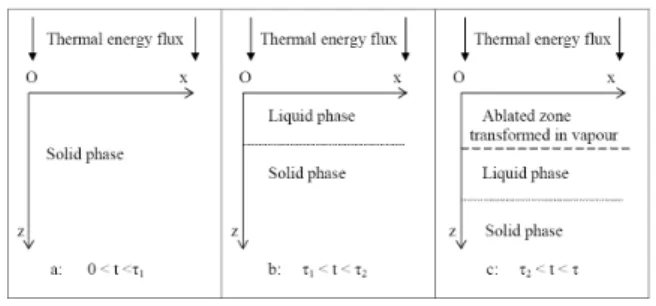
Fig. 1. 1D simulation: the thermal energy flux is applied to the infinite plan Ox, Oy, the energy dissipates only in z-axe direction. In the b and c case the thermal flux is applied on a liquid phase. At t = τ1 and at t = τ2 respectively the liquid
and vapour phase appear.
ds is an element of the surface ΓWt, −→r ∈ Ωtand s ∈ ΓWt.
A finite element method is used with moving bound-aries and ablation to simulate the time evolution of the solid liquid limit and of the liquid vapour limit. When a node enthalpy is higher than the vaporisation enthalpy this node is removed and the energy flux is transmitted to the next liquid (or solid) node.
2.1 1D simulation
The figure 1 summarizes a method detailed in the paper of Rossignol [1]. The surface energy flux W applied on the plan surface Ox, Oy is transmitted to the material only in the z-axe direction, the time duration is equal to tmax=
τ , and we are interested only by the material evolution during this time tmax.
The time interval [0, tmax] is divided on a regular basis
defined by m.tp, with m = 0...M . Interval space [0, zmax]
is divided into N intervals on each of which is expressed the approached function:
Hhm= N X j=0 Hjmφj (4) Assuming known Hm
h functions, equation (2) leads to
the values of Hm+1 h : Z [zm,zmax] Hhm+1− Hm h τ φ(z)dz + Z [zm,zmax] a(Hhm) dHm+1 h dz dφ(z) dz dz = Z [zm,zmax] W.φ(zm).φ(z)dz (5) a(Hm
h) represents the magnitude of the derivative of
the function β(Hm
h). The element z = 0 is removed from
the computational domain when the enthalpy Hhm+1, which corresponds to it becomes greater than the enthalpy Hvap
needed for the vaporization of this element. At a moment m.tp several elements have been removed by ablation, the initial area [0, zmax] is reduced to [zm, zmax]. At t = 0
the specific enthalpy is supposed to be equal to H0 at
each point of the considered volume, in the program we considered only the points of the Oz-axe, the points with coordinate (x, y, z) present the same specific enthalpy or temperature value when z is fixed, the space and time evo-lutions are only in the z coordinate. The studied domain is limited by the coordinates z0 = 0, and z = zmax, the
second limit determines the calculated length l = zmax
-z0, and it obeys to the condition H = H0 during the
en-ergy flux duration tmax. The length domain l is divided in
3000 steps with different values, the first 2000 steps
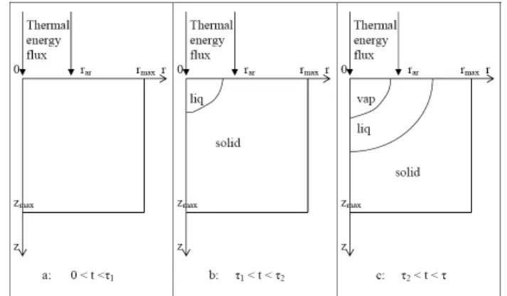
begin-Fig. 2. 2D axi symmetric simulation: the thermal energy flux is applied to a radius rarcircle surface on the plane surface of
an axe Oz and radius rmaxcylinder. The energy dissipates in
r-axe and z-axe directions. At t = τ1and at t = τ2 respectively
the liquid and vapour phase appear.
ning at z = 0 are shorter and equal to h1, than the 1000
steps finishing at z = zmaxand equal to h2. The step time
discretization tn is chosen constant and equal to Nτ with
N = 106 to avoid computation difficulties.
To compare the obtained results with experiment or with the 2D axi symmetric simulation results, we used the co-ordinate r in the plan Ox, Oy. In this case the considered volumes are cylinders with the axis of symmetry Oz.
2.2 2D axi symmetric simulation
To solve equation (1) the numerical method of finite ele-ment described in 2.1 is used, but in this case presented in figure 2 the material is a finite cylinder. The z-axe rep-resents the symmetric axe of the cylinder and the r-axe situates the points along a radius perpendicular to the axe z-axe.
The arc root is supposed motionless, this hypothesis is satisfied by the commonly admitted reasons:
- at the cathode the life time of the fragment is very short (less than 100ns),
- at the anode the spot moves slowly, or presents a short life time if it moves quickly (in the presence of a magnetic field).
Joule heating is neglected : a simple calculation shows that the produced energy in the electrode contracted zone of the current lines is very small in comparison with the transmitted thermal energy. About the enthalpy function versus temperature, the same hypothesis like in 1D simu-lation is made: the phase changes (solid-liquid and liquid-vapour) are made to be continuously on a small gap of temperature (10◦C for example).
The surface energy flux W(r) is applied at t = 0 on a cir-cular surface with centre O and radius rar during a time
tmax= τ , W(r) can be variable with the radius r and with
the time t; in the results presented in the next paragraphs W(r) is constant during the time τ . At the time t = 0 the specific enthalpy for each node of the cylinder is equal to H0, then, for t > 0 the energy is transmitted in the z-axe
and r-axe directions providing a change in the enthalpy values in each point of the considered volume. Starting from equation (2) and performing the same operations of discretization for an 1D representation, we get:
Z Ωr,z Hm+1 h − Hhm τ .φ.r.dr.dz + Z Ωr,z a(Hm h)∇dHhm.∇dφ.r.dr.dz = Z Ωr,z W.φΩr,z.φ.r.ds (6)
with φ = φ(r, z). The initial field consists of triangles K (Fig. 3), but because of the axisymmetry, a field K will be deleted when the following condition will be satisfied:
Z K Hm+1 h .r.dr.dz > Z K Hvap.r.dr.dz (7)
and the initial field is reduced to the area noted Ωr,z.
The solution of equation (6) is obtained by solving a linear system.
At the instant t = τ1 the specific enthalpy reaches a value
equal to the specific liquefaction enthalpy and the first liquid volume appears, in this case the figure 2-b shows that the surface energy flux is applied to the liquid and to the solid and one can obtain the time evolution of the depth, radius and volume of the liquid phase. At the in-stant t = τ2the same phenomena is obtained with the
va-porization enthalpy, the corresponding meshes and nodes are removed and the first vaporized volume appears, and one can obtain the time characteristic evolution of this volume.
The figure 3 shows the shape of the meshes used; in the results presented in paragraphs 3 and 4, the cylinder ra-dius rmaxand height zmaxare divided in 125 steps giving
16400 nodes. The time step is chosen equal to tmax/1000
to obtain correct results with a reasonable PC time com-putation.
In the 1D simulation case, the energy propagates only in the z-axe direction, the obtain different zones are cylin-ders (figure 4a), their volume evolution gives results about
Fig. 3. An example of the meshes used in the 2D axi symmetric simulation.
Fig. 4. Geometry of the contact with the two phases (solid and liquid), and the ablated zone by vaporization: a) 1D case: the zones are cylinders ; b) 2D axi symmetric case.
contact erosion by vaporisation and about the liquid vol-ume obtained. In the 2D axi symmetric simulation the same results appear (figure 4b), the shapes of the obtained volumes are different, this fact is due to the energy prop-agation in z-axe and in radial-axe directions.
3 Cathode arc root
At the cathode surface the classical [2] power flux balance gives:
Pi= PH+ Pr+ Pe (8)
Pi is the surface power flux delivered to the cathode surface by the ions coming from the plasma sheath, Pi is directly proportional to the cathode current density
Jc. The power flux Pe corresponds to the cooling effect produced by electron emission, generally it takes low ues [3] and one can neglect it comparatively to the val-ues taken by Pi . The surface power flux Pr dissipated by the cathode surface radiation takes also low compar-ative values; it is the result of cathode surface temper-ature which is equal to the metal vaporization tempera-ture. Under these considerations equation 8 simplifies, and the power flux PH transmitted to the cathode material is equal to the incoming power flux Pi . Using the values given by Rakhovskii [4] about the proportionality coeffi-cient necessary to obtain Piand making with J¨uttner [5-6] the hypothesis of a cathode fragment of 5µm radius and transporting a 10A current, the values obtained about Pi gives W = 5 × 10¹¹W m−2. The cathode presented results about copper are obtain with these values of W and r, the time duration tmax is taken equal to 100ns, it corresponds to the maximum cathode fragment life.
Fig. 5. The three phase energy partition versus time in the contact (1D case).
3.1 1D simulation results
The figure 5 gives the evolution with time of the energy partition. At the beginning the whole energy is used to heat the material by conduction till tcliq1D = 5.4ns , at
this time the liquid phase appears. The energy is now consumed by the two phases, the solid part decreases and the liquid part increases and reaches a maximum value at tcvap1D = 25ns , at this time the vapour phase appears.
The energy is now dissipated by vapour production, by solid liquid transformation and by thermal conduction in the liquid and solid phases. The part of energy used to the production of the vapour grows, it takes a value near 50% at the end of the spot life.
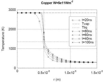
On the figure 6 the temperature repartition in the ma-terial is represented at different times. The vaporized and liquid parts appear clearly, the temperature repartition in the liquid is linear, it is the result of the imposed and constant temperaturesTvapand Tliqat each end. The
tem-Fig. 6. Contact cathode temperature repartition along z axe at different instants (1D case).
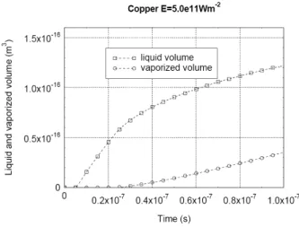
Fig. 7. Time evolution of the liquid and vaporized volume at the cathode contact (1D case).
perature distribution in the solid part is well known and classical. At t = 100ns the depth of the vaporised material is zcvap1D = 0.4µm and the thickness of the liquid phase
takes the value zcliq1D− zcvap1D= 1.6µm .
The simulation gives the time evolution of the vapor-ized and liquid zones along z axis, knowing the fragment radius rmax= 5µm, it is then possible to obtain the liquid
va-Fig. 8. The three phase energy partition versus time in the cathode contact (2D axi symmetric case).
porized volume is practically linear versus time, the slope multiplied by copper density and divided by the electric charge travelled through the fragment gives the vapour erosion rate Erc1D= 415µg/C.
3.2 2D axi symetric simulation results
At tcliq2D = 6.1ns (figure 8) the liquid phase appears and the part of energy absorbed by this liquid phase grows till a maximum value, about 40% at tcvap2D = 32ns , corre-sponding to the vaporization beginning. One can see on figure 8 that with the vapour apparition the solid energy part decreases very slowly to the value 54%, in this time interval the parts used to the vaporization and to the liq-uid phase vary in opposite direction. At the end of the fragment life the energy part in the vapour is 20%.
The figure 9 gives the temperature variations along z-axe at different times, the evolution is similar with 1D results (figure 6). After t = 40ns (figure 10) the radius of the vaporized zone presents a very slow evolution between
Fig. 9. Cathode temperature repartition along z-axe at differ-ent instants (2D axi symmetric case).
Fig. 10. Temperature repartition along r-axe, on cathode con-tact surface at different instants (2D axi symmetric case).
r40ns = 4.3µm and r100ns = 4.6µm , the liquid phase
growth is in major part directed in the z-axe direction. The length of the liquid phase in the r-axe direction on the electrode surface at t = 100ns is rcliq2D−rcvap2D= 0.6µm it represents the half of the liquid thickness in the z-axe direction.
On the figure 11 the shapes of the vaporized part and of the liquid phase are given in r,z plan, on the surface the
Fig. 11. A view along z-axe and r-axe of the cathode material vaporized and liquid phase at t = 100ns. The corresponding volumes are obtained by figure rotation along z-axe.
radius of the liquid and solid phase boundary is rcliq2D=
5.2µm . If we compare this value with the fragment radius one can see that the two values are not very different. The depth of the crater at t = 100ns is zcvap2D = 0.3µm and
the thickness of the liquid phase takes the value zcliq2D−
zcvap2D= 1.2µm.
The time evolutions of the vaporized volume and of the liquid phase are represented figure 12 the time evo-lution of the vaporized volume is quasi linear, with the slope value one obtain the fragment vapour erosion rate Erc2D= 210µm/C .
3.3 Discussion about cathode results
Roughly the two simulations give similar results (table1) in the liquid and vapour phase apparition instants and
Fig. 12. Time evolution of the liquid and vaporized volume at the cathode (2D axi symmetric case).
in the evolution of the different presented curves however the discussion about the observed differences needs physi-cal explanations. On figure 5 the vapour appears at a time tvap1D = 25ns and on figure 8 at a time tvap2D = 32ns
and the energy partitions are different, this difference is the result of the energy dissipation in three possible di-rections in the axi symmetric case. The dissipation of the energy is different in 1D and 2D simulations, this result is also visible on figure 6 compared to figure 9. The energy dissipation is more important in 1D case, this fact appears distinctly in the solid phase. The figure 10 shows the dif-ference between a cylindrical erosion (geometry defined on figure 4) and the evolution of the vaporised part and of the liquid phase; this result puts questions about the flux particle organisation [7] on the cathode surface. The curve corresponding to 20ns shows clearly that in this case the metal particle flux does not exist and that the radius of the liquid part is not equal to 5µm . The paper of J¨uttner [8] gives a copper erosion rate in the gap 10 − 300µm/C
Table 1. Comparison between 1D and 2D axi symmetric results at a 10A cathode fragment
t = 100ns
tcliq tcvap Hvap/Htot Hliq/Htot Hsol/Htot zcliq− zcvap zcvap Erosion
(ns) (ns) (%) (%) (%) (µm) (µm) (µg/C) 1D 5.4 25 50 29 21 1.6 0.4 415 2D axi 6.1 32 20 26 54 1.2 0.3 210
, the value Er1D is too large and the value Er2D
corre-sponds to this interval. The measures lead to values near 40µg/C [9] but the values are obtained by weighting con-tact electrode before and after arcing, there is a part of the vaporised material that comes back to the electrode surface or is the consequence of the anode particle flux. The cathode results show that the energy flux incoming on the cathode contact surface presents variations along the radius r and during the fragment live. The 1D simu-lation shows that 25ns are necessary to produce vapour, this time is probably too long, the fragment existing needs the presence of metallic ions to heat the metal electrode surface. Mesyats [10] shows that a 10A spot current is obtained in 0.4ns with a 0.7µm radius and a probably current density equal to 5 × 10¹³Am−2 , the 1D
simula-tion shows that in this case all the incoming energy flux is used by the metal vaporisation, there is no liquid phase and no solid heating.
4 Anode arc root
In the electric arc the anode spot collects the column elec-trons, in vacuum breakers it generally appears at high
cur-rent values (up to ×10kA ) and in other breakers working at atmospheric pressure values (or up to a multiple of 0.1M P a) it appears simultaneously with the first cathode fragment. In opposition to the cathode (several spots), the anode presents always one spot. JD Cobine and EE Burger [11] give a power density equation on the anode electrode surface:
Pa = Ja× (Va+ ϕ + VT) + Pn+ Pr (9)
Ja is the anode current density, Va the anode drop, ϕ
the material work function, Pn the result of the energy of
neutral atoms and Prthe radiant energy from the column.
Usually the two last parts of equation 9 are negligible in comparison with the first part, VT results of electron
col-umn flux it can be taken equal to 3.0V , ϕ is the material work function equal to 4.8V for copper, the values taken by Va are generally not well defined, they can be positive
or negative. The energy flux Pa is used at the anode to
in-crease material enthalpy, to provide emission of secondary electrons and to emit radiations like in the equation 8 used at the cathode. The same approximations can be made, so Pa is supposed in a first time transmitted to the anode
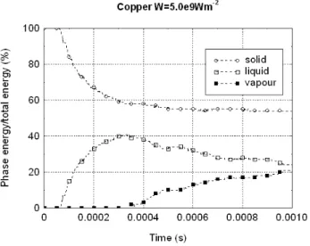
Fig. 13. The three phase energy partition versus time in the anode contact (1D case).
material. The example given here is about an anode spot carrying a 1000A current. According to the values existing in [12] and in [13] one find a radius anode spot ra = 0.5mm
and a transmitted surface energy flux W = 5×10⁹W m−2.
The arc duration ta= 1ms is a reasonable value, generally
the breakers interrupt currents in some milliseconds.
4.1 1D simulation results
Figure 13, 14 and 15 give anode results and present time evolution to similar curves in 3.1. The liquid and vapour time apparition (figure 13) taliq1D= 54µs and tavap1D=
250µs are larger than values relative to the cathode, this is the result of an energy flux divided by 100 in anode case. The vapour erosion is almost time linear (figure 15), calculated at ta = 1ms it gives the erosion rate Era1D=
414µg/C , these value is practically equal to these find in 3.1.
Fig. 14. Anode contact temperature repartition along z axe at different instants (1D case).
Fig. 15. Time evolution of the liquid and vaporized volume at the anode contact (1D case).
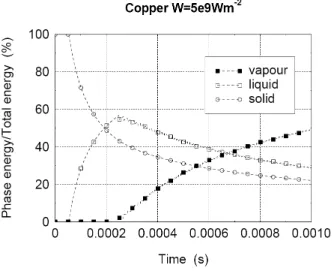
4.2 2D axi symmetric simulation results
At taliq2D = 61µs (figure 16) the liquid phase appears
and the energy partition changes, the curve relative to liquid energy part reaches a maximum value (about 40%) at tavap2D= 0.34ms, time corresponding to the beginning
of the vaporization. Then the solid phase energy part de-creases slightly from 58% to 54%, the liquid energy part
Fig. 16. The three phase energy partition versus time in the anode contact (2D axi symmetric case).
Fig. 17. Anode temperature repartition along z-axe at differ-ent instants (2D axi symmetric case).
decreases from 40% to 25% and the vapour energy part increases and is equal to 21% at ta= 1ms.
Figure 17 presents temperature distribution along z-axe at different time values, the liquid temperature may present linear evolution generally. At ta= 1ms the z-axe
liquid depth zavap2D−zaliq2D= 129µm is smaller than the
Fig. 18. Anode temperature repartition along r-axe, on con-tact surface at different instants (2D axi symmetric case).
1D simulation depth zavap1D− zaliq1D = 159µm (figure
14), the difference is 23% it is lower than cathode case. Figure 18 shows the liquid and vapour phase estab-lishment, at t = 0.2ms the maximum radius of the liquid phase is equal to 479µm .
4.3 Discussion about anode results
At ta= 1ms (figure 19), on the anode surface, the liquid
and vapour phase radius are respectively equal to 520µm and 465µm. The liquid phase radius is equal to the sur-face energy flux radius at t = 0.4ms. The corresponding volume evolution is given figure 20, the curve representing the vaporized volume is practically linear; this gives the erosion evaporation rate Era2D = 181µg/C .
Table 2 gives a comparison between the results obtain with the two simulation methods. The literature gives few values on the anode erosion rate, generally it is currently acknowledged that it is the same at cathode and anode;
Table 2. Comparison between 1D and 2D axi symmetric results at a 1000A anode arc root
t = 1ms
taliq tavap Hvap/Htot Hliq/Htot Hsol/Htot zaliq− zavap zavap Erosion
(µs) (µs) (%) (%) (%) (µm) (µm) (µg/C) 1D 54 250 49 29 22 159 45 414 2D axi 61 340 21 25 54 129 31 181
Fig. 19. A view along z and z-axe of the anode material va-porized and of the liquid phase at t = 1ms. The corresponding volumes are obtained by figure rotation along z-axe.
however the values about silver [14] are situated in the case of a half cycle 1000A current in the range 30 − 130µg/C and [15] find for the ratio Era/Erc values situated in the
range 0.4 − 0.7. With these parameters the anode ero-sion rate should be situated in the range 7 − 210µg/C , the values given by 1D simulation is too large but the 2D simulation is in the experimental range. Like in 3.3 the obtain results gives only the erosion resulting of the
vapor-Fig. 20. Anode time evolution of the liquid and vaporized volume (2D axi symmetric case)
isation phenomena, comparison with experimental result gives only limits. The anode results are probably better than the cathode results, the reason is an evolution more simple in the anode spot live. The anode only assure the continuity of the arc current by the electron collect, the radius current density is more simple with only a tran-sition zone on the anode edge, and its time evolution is probably monotone.
5 Conclusion
Simulation of the arc effect on the copper electrodes that sustained the arc discharge have been done using two sim-ulation possibilities the 1D and the 2D axi symmetric. The second simulation gives more precise results but the first was not without interest, it is more easy to use and it gives first results whose analysis confirms the validity of our hy-pothesis. The cathode fragment first nanoseconds presents a very high energy density values with only production of vapour and practically no liquid phase and no heat trans-fer into the solid. According to these assumptions, the 1D simulation gives a first approximation of vacuum arc ab-lation phenomena at small currents.
References
1. J. Rossignol., M. Abbaoui. and S. Clain, ”Numerical mod-elling of thermal ablation phenomena due to a cathodic spot”, J. Phys. D : Appl Phys. 33, (2000) pp. 2079-86 2. TH Lee and Allan Greenwood, ”Theory for the Cathode
Mechanism in Metal in Metal Vapour Arc”, J. Appl. Phys.33 , (1961) pp. 916-23
3. TH Lee, ”Energy Distribution and Cooling Effect of Elec-trons Emitted from an Arc Cathode”, J. Appl. Phys. 31 (1960) 5 pp. 924-7
4. VI Rakhovskii ”Experimental Study of the Dynamics of Cathode Spots Development”, IEEE Trans. Plas. Sci. vol PS-4, no 2 (1976) pp. 81-102
5. B J¨uttner, ”Nanosecond Displacement Times of Arc Cath-ode Spots in Vacuum”, IEEE Trans. Plas. Sci. 27 (1999) pp. 2544-51
6. B J¨uttner and I Kleberg, ”The Retrograde Motion of Arc Cathode Spots in Vacuum” J.Phys.D: Appl. Phys. 33 (2000) pp. 2025-36
7. I Beilis ”Theoretical Modelling of Cathode Spot Phenom-ena’ Handbook of Vacuum Arc Science and Technology ed RL Boxman, PJ Martin and DM Sanders (New Jersey: Noyes) (1995) pp. 208-56
8. B J¨uttner ”Cathode Spots of Electric Arcs” J. Phys. D : Appl Phys. 34 (2001) R103-R123
9. JE Daalder ”Components of Cathode Erosion in Vacuum Arcs” J. Phys. D : Appl Phys. 9 (1976) pp. 2379-95 10. GA Mesyats and SA Barengolts ”The Cathode Spot of
a High-Current Vacuum Arc as a Multiecton Phenomenon” Proc.XIXth Int. Symp. On Discharges and Electrical Insula-tion in Vacuum (Xian) vol 1 (2000) pp. 293-6
11. JD Cobine and EE Burger ”Analysis of Electrode Phe-nomena in the High-Current Arc” J. Appl. Phys. 26 (1955) 7 pp. 895-8
12. LI Sharakhovsky, A Marotta and VN Borisyuk ” A Theo-rical and Experimental Investigation of Copper Electrode in Electrode Arc Heaters: II. The Experimental Determination of Arc Spot Parmeters” J. Phys. D : Appl Phys. 30 (1997) pp. 2018-25
13. Ph Test´e, T Leblanc and R Andlauer ”A Method to Asses the Surface Power density Bought by an Electric Arc of Short Duration, and Short Electrode Gap to the Electrodes Ex-ample of Copper Electrodes” Eur. Phys. J. 18 (2002) pp. 181-8
14. R Hemmi, Y Yokomizu and T Matsumura ”Anode-fall and Cathode-fall Voltages of Air Arc in Atmosphere Between Sil-ver Electrodes” J. Phys. D: Appl. Phys. 36 (2003) pp. 1097-106
15. J Kutzner and Z Zalucki ”Electrode Erosion in the Vacuum Arc” Proc. Int. Conf. on Gas Discharge London (1970) pp. 87-94