The development of a multistage centrifugal pump for use in flow chemistry

The Development of a Multistage Centrifugal Pump for Use in

Flow Chemistry

by

Brian Yue

Submitted to the Department of Mechanical Engineering

in Partial Fulfillment of the Requirements for the Degree of

Bachelor of Science in Mechanical Engineering

at the

MASSACHUSETTS INSTITUTE OF TECHNOLOGY

June 2017

0 2017 Massachusetts Institute of Technology. All rights reserved.

Signature of Author:

Si

Certified by:

(Professor of

Signature redacted

el

x

Department of Me

/

gnature

redacted

chanical Engineering

May 26, 2017

(Klavs F. Jensen)

Chemical Engineering, and Professor of Materials Science and Engineering)

Signature redacted

JUL 252017

Thesis Supervisor

Rohit Karnik

Associate Professor of Mechanical Engineering

Undergraduate Officer

CC

w

I:

MITLibraries

77 Massachusetts Avenue Cambridge, MA 02139

http://Iibraries.mit.edu/ask

DISCLAIMER NOTICE

Due to the condition of the original material, there are unavoidable

flaws in this reproduction. We have made every effort possible to

provide you with the best copy available.

Thank you.

The images contained in this document are of the

best quality available.

The Development of a Multistage Centrifugal Pump for Use in

Flow Chemistry

by

Brian Yue

Submitted to the Department of Mechanical Engineering

on May 26, 2017 in Partial Fulfillment of the

Requirements for the Degree of

Bachelor of Science in Mechanical Engineering

Abstract

Flow chemistry is an emerging approach to chemical synthesis in which chemical processes are performed on reactants as they continuously flow through reactors. In order to drive such flows, low flow rate, high pressure pumps are used. The standard pump in use is the displacement pump. However, it tends to be expensive and produces a discontinuous flow. The goal of this investigation is to prototype a miniature multistage centrifugal pump and assess whether or not such pumps can perform in flow chemistry applications in the place of displacement pumps. This thesis explores the design features implemented in the development of this pump and how they contributed to its performance as pertaining to use in flow chemistry. Specifically, the pump was designed to be comprised of modularly stackable pump stages and to be thermochemically stable, operating without the use of dynamic seals. Ultimately, the device designed succeeded in being modularly stackable and in operating without dynamic seals. However, the target pressure rise per stage was not fully met. Moreover, testing of the pump revealed a high sensitivity in flow rate to changes in generated pressure head. Thus, it is not yet deemed a viable alternative to the current standard of displacement pumps.

Thesis Supervisor: Klavs F. Jensen

Title: Professor of Chemical Engineering, and Professor of Materials Science and Engineering

Table of Contents

Abstract

3

Table of Contents

4

List of Figures

6

List of Appendices

7

1. Introduction

9

1.1 Background on Fluidic Chemistry 9

1.2 What is Needed in a Pump 9

1.3 Current Standard Pump Design 9

1.4 Design Goals 10

2. Basics of Centrifugal Pump Theory

11

2.1 How Centrifugal Pumps Generate Pressure 11

2.2 General Character 12

2.3 Blade Curvature 13

2.3.1 Implications on Flow Stability 14

3. Design of the Pump 15

3.1 Performance Specifications 16

3.2 Design Features 16

3.2.1 Continuously Stackable 17

3.2.2 Obviating Dynamic Seals 18

3.2.2.1 Geometric Constraint without Bearings 19

3.2.2.2 Magnetic Coupling 20

3.3 Design Changes and Additional Features 21

3.3.1 Version 1 22

3.3.2 Version 2 24

3.4 Device Actuation 28

4. Testing of the Pump 32

4.1 Test Setup 33

4.2 Pre-Analysis Data Processing 35

5.

Results of Testing

38

5.1 Pump Pressure 38

5.2 Pump Flow Rate 41

6. Conclusion 43

7. References 44

8. Appendices 45

List of Figures

Figure 1: Centrifugal Pump Reduced Diagram 11

Figure 2: Centrifugal Pump with Curved Blades 13

Figure 3: Full Pump CAD Renderings 15

Figure 4: Series Coupling of Pump Stages 17

Figure 5: Magnetic Coupling 19

Figure 6: Series Coupling of Pump Stages 20

Figure 7: Version 1 Prototype 22

Figure 8: Version 2 Prototype - Exploded View 24

Figure 9: Stage Fastening - Exploded View 25

Figure 10: Version 2 Lower Half Cross Sectional View 27

Figure 11: Circuit Diagram 28

Figure 12: Assembled Circuit 29

Figure 13: Hall Effect Sensor Implementation 30

Figure 14: Pump Test Setup 33

Figure 15: Graphs of Pressure 1 and Pressure 2 with Angular Velocity 35

Figure 16: Graph of Hand Aligned Data for Four Part Sweep Test 36

Figure 17: Graph of Matlab Script Aligned Data for Four Part Sweep Test 37

Figure 18: Graphs of the Pressure Rise Ratio of the Two Pump Stages 38

Figure 19: Graph of Pressure and Flow Rate with Angular Velocity 40

Figure 20: Graph of Flow Rate with Time 41

Figure 21: Pressure Transducer Calibration 46

List of Appendices

APPENDIX A: C++ Code for Controlling the Pump 45

APPENDIX B: Graph of Pressure 2 Transducer Calibration Data 46

APPENDIX C: Matlab Script for Automatically Aligning Datasets 47

1

Introduction

1.1 Background on Flow Chemistry

Traditionally high value added chemical processes performed on low volumes of chemicals have been carried out in discrete batches. Flow chemistry is an emerging approach to chemical

synthesis where such processes are carried out while reactants flow through reactors as opposed such processes being carried out on static batches of reactant. This provides a basis for

continuous manufacturing, as well as increased repeatability, scaling, and ease of varying reaction parameters (eg. The temperatures, pressures, and times of reactions). Additionally, this

simplifies the automation of this process and allows for real time monitoring.

1.2 What is Needed in a Pump

In order to perform reactions in flow, there must be a means of generating hydrostatic pressure as well as generating regulatable fluid flow. The types of reactions being studied at the laboratory scale specifically are performed at high pressures (of order 1-10 bar) and low flow rates (of order 0.1-IOml/min). As a result, any pump which is to be used in such applications must be capable of generating a large pressure head and a low flow rate. Additionally, the reactions are performed at a wide range of temperatures and with substances which can be highly caustic. So pumps must also be resistant to a thermally, mechanically, and chemically aggressive environment.

1.3 Current Standard Pump Design

The current standard type of pump used in flow chemistry is the displacement pump.

Displacement pumps operate by discharging one or more cylinders of fluid, typically by means of an actuated piston. Pressure is easily regulated either downstream with a back pressure regulator, or by regulating the force on the piston. Additionally, under assumptions of

incompressibility, volumetric flow rate is also easily imposed by regulating the rate of change of displacement of the piston. However, in order to operate continuously, displacement pumps require two or more cylinders as well as one way valves. The use of multiple cylinders results in

a discontinuity in flow when discharging transitions from one cylinder to the next. Additionally, in order to endure the harsh environment, one way valves must be made of hard, inert materials such as highly polished sapphire. Moreover, in general, dynamic seals, such as those found between the piston and the cylinder, are more prone to leaking and to degradation due to the need for deformable materials as well as the exposure to physical wear. Expensive valves and seals, in addition to need for high precision machining results in displacement pumps being expensive.

1.4 Design Goals

The goal of this investigation is to design a miniature multistage centrifugal pump which can be used to demonstrate the viability of this type of pump technology in meeting the criteria required for use in flow chemistry. Specifically, the pump designed needs to be able to generate high pressures at low flow rates. Additionally, it needs to be impervious to the effects of thermal, chemical, and mechanical wear. Finally, in order to outperform displacement pumps, it must generate fluid flow without discontinuity and operates without the use of moving valves and dynamic seals.

2

Basics of Centrifugal Pump Theory

2.1 How Centrifugal Pumps Generate Pressure

Centrifugal pumps generate pressure by spinning a parcel of fluid at high angular velocities. As a result of the d'Alembert force acting on the fluid, a pressure gradient is created which increases

along the radius. A centrifugal pump has its inlet at the center of the rotation, where pressure is zero, and its outlet along the perimeter where the pressure is greatest.

C) b

PiG -L - P.o

R

Figure 1: In its simplest reduction, the interior of a centrifugal pump can be thought of as a spinning

disc of water. An impeller, not shown, drives the rotation of the fluid within the chamber. Assuming axial symmetry, at any given radius there is a tangential fluid velocity i resulting in a centripetal acceleration of the differential element of water. This generates a pressure difference between PO

and _P.

Under the assumption that the flow rate is negligible, all fluid velocity can be assumed to be tangential. As a result, the full expression of the acceleration a' given the derivatives of the radius r and angular velocity w reduces from: [1]

d

(1)

To:

a

_er

ac = rw2 ₍₂₎

From a force balance on a differential element at radius r, the following equation for pressure, P, can be found: d P - = pac = prw2 (3) dr Prr

j

dP

Given a trivial flow rate and a rigid impeller, o is constant with r. While this is not always a valid assumption, it holds where the flow rate is negligible. This yields that the theoretical pressure difference between the inlet and a point at radius r to be:

1

p

2.2 General Character

From equation 4 it can be seen that pressure increases linearly with the fluid's density, p, and quadratically with both the impeller's angular velocity and with its radius. The flow rate out of centrifugal pump, where still considered small, is governed by the backpressure and viscous drag of the downstream system. Geometrically speaking, the volumetric flow rate out of a pump is equal to the radial velocity at r = R multiplied by the outlet area. Thus, a pump for operation at higher flow rates will require a larger depth, b, than one for use at lower flow rates.

One of the major benefits the centrifugal pump has over the displacement pump is that it can be stacked in series without encountering phase interference. As a result, the pressure of a

centrifugal pump system can be increased without changing the flowrate by connecting the outlet of one pump to the inlet of another, thereby summing their pressure head. Thus, the range of

operating pressures for a system of centrifugal pumps can be modularly increased and decreased

by adding and removing pumps in series.

2.3 Blade Curvature

Removing the assumption of negligible flow rate, blade geometry begins to have an effect on pump pressure and, accordingly, flow stability.

V

Figure 2: A less simplified examination of the centrifugal pump reveals how fluid flows through the pump as well as how it rotates around it. U denotes the velocity of the impeller and V denotes the velocity of the fluid.

P

The equation for volumetric flow rate,

Q:

Q

Q

ve (r) =

COO

27r ((r))

21rrb

Ignoring losses, conservation of energy can be used to calculate the theoretical maximum pressure rise generated by an impeller. The Euler Turbine Equation: [3]

V = h(P -V - 'U -Pi1) = pQ (U2 * v02 - U1 * vi) (6)

W denotes rate of work being done on the fluid by the impeller blade. Given that the inlet

velocity, v, is purely radial the equation reduces to:

W = pQU2 * V02

Work rate, W, also equals the rate of change in energy of the fluid:

1

W=APQ+

IpQ(v

2

In the case where the fluid velocity is throttled down from V2 to 0 without contributing to the static pressure, W will decrease by 1p(v22 - V1

2

). These two work rate equations yield:

1

APQ= W -- pQ(v22 - V12)

2

Q

Pr

Pi

p

2or

(8)

Q,

171 = 0 v= wr P- =ppo~- 2)2 or

PrPL=(

₂

2.3.1 Implications on Flow Stability

Under such small flow rates, Eq. 8 yields the same result as Eq. 4. It is difficult to predict how much kinetic energy is lost in throttling down the fluid velocity. Likewise, regarding the force balance method of solving pressure rise, it is difficult to predict how much momentum due to tangential velocity is not throttled but converted into pressure rise. Regardless, Eq. 8 makes it evident that the blade angle, fl, has an effect on the pressure rise proportional to the flow rate. Thus, three different behaviors can be achieved by varying the blade angle. (1) Forward curved blades will result in an increase in pressure with an increase in flow rate. (2) Radial, or straight, blades will result in no dependency between pressure and flow rate. (3) Backward curved blades

will result in a decrease in pressure with an increase in flow rate. This behavior can be favorable as it results in greater stability of pressure and flow rate as either one is perturbed.

3

Design of the Pump

-

I IV~

(C)

(D) (B) +

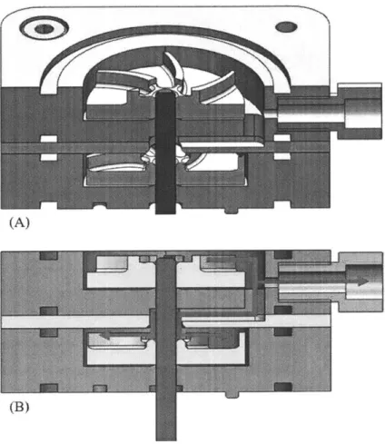
Figure 3: (A) and (B) are respectively a diagonal view and front cross sectional view of the full three stage pump system. (C) and (D) are respectively a diagonal and top views of a single stage of the pump. The beige protruding pieces are pipe fittings. The red component is the motor (A & B). The blue rod is the sapphire turn shaft (B & D). The light grey discs are the impellers (B, C, & D). Fluid enters the top, by the beige fitting, and exits the third stage down via the second fitting on the

3.1 Performance Specifications

The target specifications for this pump are that it has to generate a pressure difference of 1 bar per stage at a low flow rate which can be throttled between 0.1 and 10 milliliters per minute. Moreover, it has to be chemically compatible and mass producible for a low cost compared to displacement pumps. In order to meet the pressure requirement, an impeller diameter was chosen which, in conjunction with the motor chosen, is able to meet double the required pressure of 1 bar per stage. Specifically, the impeller was chosen to have a 12mm radius which, from equation 4, will reach 1 bar per stage at 11,300 rpm. It is designed with backward curved blades for increased flow stability. The motor chosen to drive it is a 12V DC RS-550 motor with a no load speed of 19,300rpm and a stall torque of 45Ncm. It has a theoretical maximum power output of 450W at 9,650rpm operating at 38A. However, the motor controller board chosen to drive it is a

13A Cytron, so the maximum power output is limited to 156W. Thus, at 11,300rpm, this

board-motor combination will be able to produce a maximum theoretical torque of 13.7Ncm.

3.2 Design Features

In order to meet the design requirements, features were designed in order to make the pump modularly stackable, obviate the use of dynamic seals, and allow for proper assembly and maintenance. Once the rough numbers were confirmed, the pump was designed in pieces via Solidworks®, a computer-aided design software, and outsourced to be CNC mill machined via Proto Labs®, a rapid prototyping company. The machined parts were designed to be

manufactured out of a thermochemically stable perfluorinated polymer such as PTFE (Teflon®) with the load bearing members being made of standard geometry A1203 crystal (artificial

sapphire/ruby). Of chemically stable materials, Sapphire was chosen for its high strength and hardness, as well as for its low coefficient of friction. This low coefficient of friction and high harness are essential to the longevity and performance of the designed sleeve and cup bushings. Additionally, fluorinated ethylene propylene o-rings were chosen to maintain static seals. Standard fasteners were chosen to attach different parts of the pump where isolated from the pump's contents. That said, for mechanical stability and reduced cost, parts were prototyped in inexpensive alternatives to their thermochemically stable counterparts.

3.2.1 Continuously Stackable

One of the primary benefits of the centrifugal pump is the potential to stack multiple stages

inlet-to-outlet in order to step up the pressure. This is the central design concept, and much of the design has been built around it. The basic concept is that the outlet of the first pump feeds into the inlet of the second pump. Where this can be accomplished with independent pumps connected by hoses, in order to incorporate these pumps into a single device, these were

designed to assemble axially aligned pumping stages driven by a single turn shaft. As a result, all the pump stages are designed with the turn shaft located at the center. The impellers are mounted onto the shaft at each stage via an interference press fit.

(A)

Figure 4: Two different angle perspectives are shown of a cross section of a pair of adjacent pump

stages. In blue is the central turn shaft, in off-white is the impeller, and in beige is the fitting of the outlet connection. A red arrow has been added to (B) to denote the possible paths the fluid can flow along, specifically (1) out the beige fitting and (2) into the inlet of the lower stage. In this thesis, the blue-grey piece with a depression for the impeller is referred to as the basin, and the pale grey piece in the center is referred to as the lid.

The pump is designed to be comprised of a series of axially aligned, stacked pieces sealed together with o-rings. While the o-rings are not displayed in the CAD rendering, the grooves for them are, specified for static sealing against an internal pressure (Figure 4) [4]. The flow path from one stage to the next is machined out of the bottom of the basin and the top of the lid. It runs from the outer perimeter of the earlier stage's basin to the center of the later stage's lid. While part of the basin is used as a sleeve bushing to physically constrain the axle, the flow path at the opening of the later stage is widened around the axle, such that fluid enters the later stage symmetrically about the axle. In order to assure alignment between the flow paths of an adjacent basin and lid, alignment nubs and sockets were added to both and can be seen protruding from the bottom of the basin in figure 4. Finally, a -28 bottom tapped outlet is placed on the side of each basin connecting to the outlet channel. This accommodates a standard fitting and allows for a flow path to be designated from any stage, which allows for easier testing of the pump. (Note that adjacent stages are mounted 900 offset from one another, so the fitting is only visible on the upper stage of figure 4) All unused outlets are plugged to prevent depressurization and leakage. Future iterations might include two different styles of basin, one without an outlet for use as a pressure step, and one with an outlet and no flow path to the next stage to act as the final outlet stage of any stacked pump system.

3.2.2 Obviating Dynamic Seals

One of the unique challenges in developing a pump for use in flow chemistry is the need for the pump to withstand extreme temperatures and chemicals. This becomes most difficult to resolve in dynamic seals such as those found where a shaft enters a pump from an outside environment. Dynamic seals intrinsically require compliant materials, such as o-rings to prevent leakage. Such thermochemically stable, compliant materials tend to be expensive and hard to machine.

Moreover, at the interface between a stationary hole and a rotating shaft, these materials are subjected to extreme mechanical wear. Prior testing with o-ring seals resulted in the o-rings having a very short functional life before failing. Similar issues made the use of peristaltic type pumps inviable. The solution explored here is to obviate the need for dynamic seals by means of a fully enclosed turn shaft which does not penetrate the surface of the pump system. Such a shaft is driven indirectly via a magnetic coupling. A later design might have the shaft itself act as the rotor of a brushless motor and be driven directly by external magnetic coils.

4

3.2.2.1 Geometric Constraint without Bearings

The shaft itself is axially aligned by means of a sleeve bushing at one end and a ball joint at the other. The coefficient of friction between PTFE and A1203 is assumed to be low (-0.05-0.2 though specific numbers are difficult to find), so the friction due to such a surface interaction is predicted to be unproblematic. However, sleeve bushings are not impervious to leakage, which is

why they cannot be used to pass the shaft from the exterior to the interior of the pump. That said, assuming the viscous drag along the back flow path is much greater than that of the forward flow path, the pump will still be able to generate a standing pressure head, and such leakage between

adjacent stages will simply contribute to pressure losses and inefficiencies without fully compromising the pump's behavior. In this regard the forward flow path from one stage to the next is 2mm x 2mm whereas the bushing around the shaft was reamed with a 3.1877mm ream to accommodate a 3.04mm shaft, resulting in a 9.8mm x 0.07mm back flow path.

Where one end of the shaft is constrained from translating in 2D via a sleeve bushing, the other end is constrained from translating in 3D by means of a ball joint. Unlike in typical

implementations of a ball joint, which require for the ball to be semi enclosed by the joint, this ball joint is held into the cup bushing by the magnetic coupling used to drive the shaft (Figure 5). As a result, there is minimal contact between the ball and the cup bushing. While it is possible for the ball to be lifted from the cup, the magnetic coupling force restores contact again, and the conical depression ensures centering it.

(A) (B)

Figure 5: (A) Depicts that the magnetic coupling between the motor shaft, below in grey, and the

fluids from within the pump to the exterior. There are four magnets per side, depicted in beige, though only two are visible in this cross sectional view. They are arranged in alternating north-up, south-up orientations. (B) Depicts a close up examination of the ball and cup joint between the sapphire balls, denoted in blue, and the small conical depressions in the interface.

The vertical alignment of the impellers is maintained by means of point contact interactions between the impellers and the basins. The base of each basin beneath the impeller rises up in a conical fashion up to the bottom of the impeller (Figure 3 -B). As a result, the contact force between the impeller and the basin occurs over a very small area at a small radius of 1.6mm, thereby reducing the losses due to friction induced resistive torque.

3.2.2.2 Magnetic Coupling

The magnetic coupling between the motor shaft outside the pump and the impeller shaft inside the pump is developed by two sets of four magnets arranged in alternating north-up, south-up orientations. By alternating the polarity in this fashion, there are four phases opposed to the two which would be there if they had been arranged north-up, north-up, south-up, south-up. This results in a magnetic coupling which decays more rapidly with vertical distance, but restores more strongly with variations in angle.

(A) (B)

Figure 6: (A) is the magnetic coupling head for the impeller shaft enclosed within the pump. (B) is the magnetic coupling head for the motor shaft outside the pump. The magnets chosen are

%"x/4" nickel coated N48 neodymium magnets. Red indicates the north end of the magnet, and blue indicates the south end of the magnet. In the center of each magnet holder is a sapphire ball used for alignment as seen in figure 4 - B.

The magnetic coupling head for the impeller shaft is designed to isolate the magnets from the chemicals being pumped. As a result, the magnet holder fully encases the magnets and seals them in with an o ring and cap. The shaft, indicated in blue, is interference press fit into the cap which mechanically couples with the magnets via nubs and sockets (Figure 4-A & Figure 5-A). In contrast, the magnetic coupling head for the motor shaft is not exposed to chemicals, so the magnets are left exposed. In order to reduce the coupling distance as much as possible, the magnets are interference press fit into the face of the magnet holder with no additional material between them and the solid interface. The motor shaft, indicated in dark grey, is interference press fit into the other end of the magnet holder (Figure 5-B).

3.3 Design Changes and Additional Features

Two physical prototypes were made after developing the initial concept. The first one was machined and tested. It was used to inform major design changes for the second one. The second

was likewise machined and tested. It was used to provide minor modifications for the final version. Some of the components of the second iteration were reused from the first one, so it differs slightly from the actual design.

JMMI-3.3.1 Version 1

Figure 7: (A) and (B) are respectively a diagonal view and a front cross sectional view of the version

1 prototype. The beige protruding members represent the pipe fittings. The flow path, sapphire axle (in grey) and magnetic coupling can all be seen in the cross sectional view (B).

The main internal geometry currently being used was developed in Version 1. That said, for actual prototyping only two stages were made as opposed to three. It was shown to pump water in proof of concepts test in which the shaft was directly driven and allowed to leak. However, Version 1 was prototyped in aluminum for its ease of machining and high strength compared to plastics. This proved problematic in two ways. First, there was considerable binding between the

steel axle and the aluminum sleeve bushings to the degree to which flecks of aluminum were found in the pump upon disassembly. Second, there was considerable parasitic drag due to eddy currents as the magnetic field was changed through the highly electrically conductive aluminum. While aluminum was never intended to be the final material used, due to its lack of chemical compatibility, these issues did prevent testing of the efficacy of the magnetic coupling until the pump was prototyped in plastic.

A lasting design modification was inspired by Version 1 concerning how the stages of the motor

are fastened together. Version 1 had the all of the layers held together by four long axially oriented screws with nuts. While this was successful at compressing the o-rings between each layer, it presented a problem in assembling the pump. Specifically, it resulted in binding between the impellers and the housing. The problem arose because the o-rings add to the spacing between stages prior to being compressed when the screws are tightened. Because the impellers are mounted on the turn shaft by means of interference press fits, when assembling consecutive layers, the spacing between impellers was greater than that of the final spacing of the stage housings. Thus, when the four screws were tightened after fully assembling the turn shaft, impellers, and stage housings; the o-rings compressed, causing the lid of each stage to press down upon the top of the impellers. The solution to this was to have each stage mounted onto the stage above it before the next stage was added.

-- - - .I

3.3.2 Version 2

Figure 8: This is an exploded view of the physical Version 2 prototype. All the parts are laid out in

approximate relative position to the other parts of the assembly. All machined pieces are nylon (in black) except for an aluminum lid (in silver) and a polycarbonate top viewing plate (in frosted clear).

Version 2 was designed from Version 1 with modifications to resolve the observed problems, as well as with a few additional components and features developed independent of the testing of Version 1. Regarding the former, the aluminum was mostly replaced with nylon in the exception of the stage lids which were reused from Version 1 (Figure 8). In order to have each stage

mounted and secured consecutively the four long screws were replaced by countersunk short screws which connected adjacent stages. In order to reduce the number of design changes, two screws held each layer, being placed at opposing corners of each stage and mounting into tapped holes in the stage below. For this reason, each stage is 900 offset from the layer above, such that the two countersunk through holes of the upper layer align with the two tapped holes of the layer below (Figure 9).

Figure 9: This is an exploded view of two adjacent stages. It can be seen that the upper stage is rotated 900 clockwise from the lower stage, allowing for its two screws to align with the two available tapped holes below. Countersinking the holes allowed for the screws to be flushed when tightened, thereby preventing them from interfering with the fit.

It was observed from the Version 2 prototype, that given the stiffness of the nylon and its

viscoelastic creep behavior, the force required to compress the o-rings between each layer is

sufficient to bend the nylon and cause separation at the corners not attached. This behavior is

exacerbated by the fact that adjacent corners are loaded in opposite directions. As a result, there has been a small degree of leakage out of the pump, which complicates testing through the risk of electrical short circuit and through the introduction of air bubbles into the pump when not running alone. The conceived solution to this is to increase the number of fastening points between adjacent layers from two to three or four. Alternatively, the full length screws might be reintroduced. In redesigning this, finite element analysis should be used to verify that there will not be any significant separation.

For prototyping purposes, Version 2 encountered issues with the chemical stability of the materials used. Specifically, the steel turn shaft began to rust and needed to be frequently polished and greased in order to prevent it from binding in the nylon bushings. Additionally, nylon is slightly water absorbent resulting in mild swelling and of the nylon becoming slightly more gummy under use. These type of behaviors should be considered in the material selection and designing of the final version. That said, as far as chemical compatibility goes, PTFE and

A1203, however, should be stable with the chemicals to be used.

Some additional design features were added to Version 2. One of which is a flow inlet-outlet pair in the magnetic coupling chamber. This flow path is included in order to allow for a nonintrusive cleaning of the entire pump by means of purging it with a suitable solvent such as acetone (Figure 10). Without it, small volumes of fluid are liable to leak into the magnetic coupling chamber over time and potentially precipitate and interfere with the mechanical operation or react with future chemicals used in the pump. Another design change was a motor mount. This piece holds the motor in fixed alignment with the rest of the pump, ensuring that the magnetic head does not tilt off axis and rub against the interior of the magnetic chamber (Figure 10). This piece is also designed to hold the hall effect sensor which is used to monitor and control the motor speed.

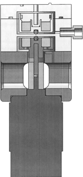
Figure 10: A front cross sectional view of the lower half of the pump. The fitting, in beige, connects

to the purging outlet of the pump. There is an inlet, not show, at the top of the magnetic coupling chamber. Additionally, between the magnetic coupling chamber (in light grey) and the motor (in red) are two pieces. The one in the center is a shaft coupling, used to connect the motor shaft to the motor's magnetic coupling head. On the outside is the motor mount. This holds the motor in alignment with the pump and is held to both the motor and the pump by screws.

3.4 Device Actuation

The pump is powered by a 12V DC RS-550 motor with a no load speed of 19,300rpm (2,020 rad/s) and a stall torque of 45Ncm. The motor is powered by a 12V 30A Regulated DC Power supply via a 13A 5-25V reversible Cytron DC motor controller which receives a pulse width modulated input. Controlling the motor controller is an Arduino Nano (ATmega 328

microprocessor chip).

H alE Sensor

Ginund

MW E

~

Figure 11: A circuit diagram of the pumps' electronic components. Small modules, such as RC

low

omitted.

voltage

(A) (B)

Figure 12: The solder to, perforated protoboard used to connect all the components needed to drive

the pump. The Arduino Nano, board power switch, rotary potentiometer, and emergency interrupt switch are shown in (A). The motor controller board is shown in (B). The motor, hall effect sensor, and power supply are not shown.

Fundamentally, the whole process revolves around the potentiometer being used by the operator to specify the desired voltage to drive the motor with. A unipolar hall effect sensor was added to report the motor speed and to give the opportunity for closed loop control. Hall effect sensors operate as magnetically triggered transistors, such that when acted upon by a magnetic field of correct orientation and sufficient strength, they complete the circuit. Otherwise, they open the circuit. This opening and closing of the circuit is used here to signal when the orientation of a magnet changes. The hall effect sensor is mounted in the top of the motor mount, near the rear end of the motor's magnetic coupling head (Figure 13). As a result, every time the head rotated one full revolution, the four magnets trigger a low-high-low-high signal. A basic RC low pass filter is placed in parallel with the sensor to prevent false triggers due to noise.

(A) (B

(C)

Figure 13: The hall effect sensor is placed on the top of the motor mount, right behind the motor magnetic coupling head. (A) shows a top view of the sensor placement. (B) is a side view and shows the simple RC circuit used to low pass the incoming signal. (C) shows an early full implementation in which the hall effect sensor was used to measure the motor velocity.

The hall effect sensor is used to measure motor speed by measuring the average time it takes for the magnetic field to switch directions. Generally speaking, there are two ways to determine the frequency of a periodic motion. The first is to measure how many cycles occur over a certain length of time, and the second is to measure how much time passes over a certain number of

cycles. In the case where the resolution of cycle measurements is higher than the resolution of time measurements, the first will yield a higher resolution reading. However, in the case where the reverse is true, the second will yield a higher resolution reading. As the time resolution of reading an ATmega328's clock is of order I [is, and the resolution of measuring the magnet's position is of order 100 s minimum (at maximum motor speed), the second method was chosen.

Thus, the code was written so that the Arduino begins counting time when the motor magnetic coupling induces a positively oriented magnetic field and continues counting time until the magnetic field has reversed polarities a predetermined number of times. This time is averaged over the number of times the polarity switched and then scaled by a factor of two (the number of north-south pairs in the motor magnetic coupling). This method of measuring frequency leads to a problem, however, where the motor becomes prone to stalling, as no other operations can be performed while the Arduino is measuring time. Thus, any stall prevention measures cannot be based on the system's ability to read when the frequency reaches zero, because as the frequency approaches zero, the time it takes for the motor to complete the required number of rotations diverges to infinity. This is resolved by adding a conditional statement, such that should the time between the motor switching poles exceed a certain threshold, the frequency measurement is be arrested and a stall is declared. In this way, while a fully automated, closed loop controller was not needed for this stage of development, the sensor was used for some forms of feedback control such as stall detection. (Full C++ script in APPENDIX A) Should a closed loop speed controller be need in the future, the frequency measurement from the hall effect sensor should be useable to inform modulation of power.

4

Testing of the Pump

In order to assess performance of the pump, several characteristics needed to be measured. Specifically, the pressure rise at each stage, as well as the flow rate through the pump needed to be measured at different impeller speeds. While standard pump characterizations involve plotting pressure as a function of flow rate for different impeller speeds, this type of comprehensive characterization was not within the scope of this investigation. Rather, the goal of testing was primarily to demonstrate a linear scaling of pressure with the number of stages and to see if the pump met the other design criteria.

4.1 Test Setup

All tests were performed with water at standard temperature and pressure.

flow Meter EI[ffII-C Messi Back Pressure

Pressu Stage I Pressure Stage Gure RexuLat r

(A)

Water Reservoir

Figure 14: This is the test setup. (A) shows the flow path of the fluid with regard to all the elements

which come into direct contact with the fluid. All components which do not directly contact the fluid, such as the electronics, are omitted. For ease of viewing, the pump stages are denoted as two separate entities Pressure Stage 1 & 2. (B) is a photograph of the actual test setup in lab. In addition

to the electronics, (B) contains the priming pump where (A) does not. The priming pump is needed to start the pump but does not have an effect after the pump begins moving fluid.

33

I

Before testing the full system, the test components were independently tested. The flow rate monitor (Sensirion SLI) was found to report maximum flow rates of 20-30mIminute with a manufacturer rating of up to lOmL/minute. It was observed, however, that for flow rates higher than 20-30mUmin, the sensor saturates and begins reading lower and lower values for the flow rate. The pressure sensors were calibrated using regulated inert gas pressure. The pressure 1 mechanical pressure gauge was found to be accurate to its degree of precision (1/2PSI), and the pressure 2 electronic pressure transducer was characterized between 0 and 18PSI in order to equate the analog voltage read to a pressure value. The data was well fit with a linear relationship

(APPENDIX B). The single component which was not tested was the dome-loaded back pressure

regulator, and this may have resulted in some of the unexplained observed behaviors.

In order for the pump to operate, it first has to be primed with water. The goal of doing so is to remove all air bubbles from the pump. As the pressure head of the pump is linearly dependent on the density of the fluid being accelerated (Eq. 4), the inclusion of too much air risks causing the pump to lose pressure and start free spinning. The pump is primed by forcing water through via the purging outlet at the bottom of the magnetic coupling chamber. Filling it from the bottom up helps to purge out the air bubbles. However, even after thorough purging, it was still observed through the transparent top, that air pockets would form at the center of the impeller during operation. Due to the pressure gradients formed about the impellers, the air pockets were located at the centers of the impellers. It is yet unclear at what point the air bubbles entered the pump whether through the poor seals between layers or by the accumulation of gas originally trapped in the water. It is unlikely that the bubbles were formed entirely due to cavitation, as they did not disappear upon stopping the pump. As a result, the pump had to be periodically stopped and purged between tests to prevent gas buildup. This will have to be investigated further and resolved with a better sealed pump and possibly a degasifier.

It was also observed during testing that at a certain velocity the magnetic coupling would break. This occurred consistently around 10,000rpm. When this happened, the motor velocity would jump, and the impeller velocity would drop. No formal calculations had been made regarding the maximum velocity the magnetic coupling would support before viscous drag and contact friction

would force decoupling. Due to decoupling, the impeller does not reach the theoretical minimum velocity of 11,300rpm required to generate 1 bar per stage.

4.2 Pre-Analysis Data Processing

In order to test the pump, two types of data were collected. The first was a series of discrete measurements of pressure 1, pressure 2, and the flow rate for a given motor speed. This was conducted for two different back pressures. As the pressure 1 gauge did not have an electronic readout, data had to be taken in discrete measurements. This data was taken in order to assess pressure head generated by each stage.

Pressure and Flow Rate Data from Back Pressure

1

S

Pressure and Flow Rate Data from Back Pressure

2

Figure 15: The measurements of pressure 1, pressure 2, and the flow rate are plotted for different motor velocities with the motor speed as the x axis. The decrease in measured flow rate at higher motor speeds (as seen in the data with back pressure 1) might be due to saturation of the flow sensor.

10 8 6 4 2 0 a. V In In a, a.

S

In addition to this data, there were tests recording pressure 2, the flow rate, the impeller velocity, and the potentiometer input across a continuous sweep of impeller velocities. For this second set of tests, the test setup unfortunately had data being collected on three independent devices with independent clock times and sample rates, though only one of the clock time measurements was recorded (from the flow rate sensor). As a result, aligning the data had to be performed using characteristic behaviors of the data. Specifically, the breaking of the magnetic coupling was used to align the different data sets. In each data set where the shafts decoupled, the pressure and flow rate measurements experience an abrupt decrease to zero. Similarly, the motor speed reading experienced an abrupt increase. Under the assumption that this transition occurs at the instant the shaft decouples, for all measurements, this feature was used to align the data sets. Tests were run such that each data set included several sweeps from stationary until magnetic decoupling in order to allow for the data to be aligned.

Hand Aligned Data from Four Part

AM a *a 4j sw o f , I M -

~az:~-MW

Sweep Test

-Figure 16: Pressure 2, flow rate, potentiometer, and frequency data taken from a set of data with four sweeps in it and plotted against a time axis. The data sets were hand scaled with time to align with each other, and were scaled in value for improved visualization. For this reason, the axes were left unlabeled.

Pressure 2 Flow Rate Potentiorme RPS

A Matlab script was written to detect each time the data exhibited the characteristic change and

generate a linear least squares fit between those times and the ones exhibited in the flow rate data (the flow rate data was chosen as the standard as it, alone, was collected with computer clock time stamps). The fit parameters were used to linearly time scale the other data sets such that they aligned with the flow rate data set. Finally, as the data was collected at different sample rates, in order to make sure that each sensor had a data point for each time stamp, each data set

was recreated by linearly interpolating new data points from between the ones collected. This was performed so that the different data sets to be able to be compared to each other, specifically so that the pressure and the flow rate could be plotted against the motor speed.

Script Aligned Data from Four Part Sweep Test

% 0 . 4 Pressure 2 Flow Rate Potentiometer RPM N --0 10 * . . 20 30 40 Time [s] 50 60 70

so

Figure 17: Pressure 2, flow rate, potentiometer, and frequency data taken from a set of data with four sweeps in it and plotted against a time axis. This is a plot of the same dataset as in Figure 16, only this one was aligned completely by the Matlab script (APPENDIX C). Three resulting differences are that: (1) The x axis corresponds to the actual time in the experiment (all data is time scaled to match the flow rate time data). (2) The data points for Pressure 2, Potentiometer, and RPM were linearly interpolated from the previous data to correspond to the time intervals from the flow rate data. (3) The mean value scaling resulted in different scaling factors for each data set than in figure 16.

5

Results of Testing

There are two primary criteria which must be met by this pump. The first is that it has to be able to generate a stackable pressure rise on the order of 1 bar per stage. The second is that it has to be operable at precisely set low flow rates.

5.1 Pump Pressure

Examining the discrete data collected for the pressure of stage 1 as well as stage 2 (as shown in figure 15) it can be seen that both stages generate a similar pressure drop for different motor speeds. Plotting the ratio of the pressure rise over the second stage and the pressure rise over the first stage yields the following two plots, one for each back pressure used:

Ratio of Pressure Rise with

Impeller Speed - Back Pressure

1

Ratio of Pressure Rise with

Impeller Speed - Back Pressure

2

Figure 18: The ratio of the pressure rises at each state was calculated by dividing the difference in pressures 1 and 2 by pressure 1. This was plotted for different impeller speeds. The data is split into two categories, dark blue being the pressure ratio where there was zero fluid flow, and light blue being the pressure ratio where the fluid was flowing.

'-I a. 3.5 3.0 2.5 2.0 1.5 1.0 0.5 0.0

Given that the limited resolution of the mechanical pressure gauge (0.5PSI), it is difficult to draw any precise conclusions, especially where the pressures near zero. That being said, from the measurements with back pressure 2, the ratio of the pressure rise of stage 2 to stage 1 appears to be 1:1 until the fluid begins to flow at higher pressures. There the pressure rise of the second stage becomes increasingly greater than that of the first stage. While this could be the effect of the increasing impeller speed, the fact that the onset of this transition occurs earlier inn the back pressure 1 data, where flow also begins earlier, makes it seem less likely to be the case. Thus, it could either be the effect of the increased flow rate or the result of the mechanical pressure sensor saturating. Examination of equation 8, reveals that the pressure rise across a stage has a

porcot(flr)

Q

21rrrb

the same speed, and pumping the same fluid, where no mass is gained or lost the change in volumetric flow rate,

Q,

With regards to the maximum pressure achieved by the pump, the rpm sweep data should be considered. Maximum pressure of the system occurred immediately before the breaking of the magnetic coupling. Across different tests, the magnetic coupling broke around 10,000 rpm with fair consistency.

Pressure and Flow Rate with Impeller

Velocity

-2.

Angular Velocity [rad/s]]

Figure 19: The same pressure 2 and flow rate data as in figure 17 has been plotted against the

impeller velocity. All data points from times where the angular velocity was zero were removed. Additionally, all data points from times after the decoupling of the magnets were removed as well. The pressure data is separated into pressure 2a (the pressure 2 measurements taken before any fluid flow) and pressure 2b (the pressure 2 measurements taken after fluid began to flow). Quadratic curves have been least squares fit to both sets of data.

From testing, the highest pressure repeatedly observed was around 0.8*105Pa (12PSI)

immediately before the magnetic coupling broke at around 1050rad/s (10,000rpm). This pressure averages a mere 0.4* 105Pa per stage which falls well below the required 1.0* 105Pa per stage. However, the magnetic coupling broke before the theoretical minimum angular velocity required to generate 1 bar of pressure, so the performance loss might be found there. Additionally this pressure was measured with a considerable flow rate,

Q,

Examining the no flow pressure curve, an estimate of the pump efficiency can be made for use in predicting the required impeller speed to reach the target 1 bar of pressure per stage. Near the

flow transition point, the pressure was 0.5* 105Pa with an angular velocity of 700rad/s. Additionally, from examining the average pressure at low velocities it is apparent that the pressure gauge was not calibrated to zero. Examination of pressure data for when the impeller

velocity was zero reveals that the actual zero pressure point was around -0.1 * 105Pa (-2PSI).

Normalizing to this, the pressure rise is 0.6*105Pa at 700rad/s. Eq. 4 predicts a theoretical pressure of 0.7*105Pa (0.35* 105Pa per stage) at 700rad/s for the no flow pressure condition, revealing the pressure generated to be 90% of what was predicted. Note that this not the pump's energy efficiency, as the pressure calculation assumes an initial 50% loss in energy efficiency due to the throttling down of the fluid's tangential velocity (Eq. 8). Assuming the 90% pressure

generated holds true for higher pressures as well, the corrected impeller velocity needed is roughly 1,250rad/s (11,900rpm). This is not too far beyond the 10,000rpm currently reached before decoupling.

5.2 Pump Flow Rate

Flow Rate with Time for Impeller Speed

40

Sweep Trials

Figure 20: The flow rate data measured at each time interval during the course of sweeping the

motor velocity from zero to decoupling three consecutive times.

The other performance criterion of the pump is its ability to be operated at low, precisely set flow rates. Examining figure 19, there is an abrupt change in flow rate from approximately zero to more than 20mUminute (over twice the maximum rated flow rate for the sensor). Examination of the flow rate about this point reveals almost zero transition region. There are no data points between where the flow rate is zero to when it reads 20mL/min, and data points are collected 20

times a second (Figure 20). As a result, while the data collected is inaccurate for describing the precise flow rate out of the pump, it reveals that the flow rate in the test setup was highly

sensitive to slight changes in impeller speed. It is possible that this was the result of the dome-loaded back pressure regulator being faulty, or of the system, as tested, lacking sufficient sources viscous drag. This will have to be explored in a later investigation. Otherwise, the discontinuity in flow rate did not demonstrate that this pump can properly throttled to achieve a precise flow rate.

5

Conclusion

This investigation was conducted in order to assess whether or not a stacked impeller pump might be effectively used to drive flow chemistry processes. It was concluded that stacked impeller pumps can be miniaturized while maintaining the ability to stack pressures.

Furthermore, the developed prototype was able to achieve pressures near what was desired such that with some modification it should satisfy the pressure requirement. In addition to this, solutions were developed to obviate the use of dynamic seals, allow for the implementation of closed loop feedback control, and make the pump stages modularly stackable. However, testing of the pump failed to demonstrate the ability to operate the pump at finely specified low flow rates. Moreover, rapid transitions from zero flow to high flow indicate that stacked impeller pumps may be intrinsically ill suited for operations requiring precise flow rates, such as those in flow chemistry, which use the flow rate to enforce reaction times. Further investigation of this matter is required in order to definitively draw such conclusion. Ideally further testing will be performed with the same type of flow path which the pump will be used for in flow chemistry processes.

Other work to be continued in developing the pump involves changing the way pump layers are fastened together to prevent leakage due to part deflection. The pump will need to be prototyped and tested in chemically compatible materials such as PTFE and A1203 in order to be used for

chemistry. Also, a stronger magnetic coupling should be developed in order achieve the pressure rise per stage. Finally, a closed loop feedback controller should be written once the pump is fully characterized.

Recommendations on further study of the pumps behavior include mapping its pressure, flow rate, angular velocity curves; measuring its power efficiency; exploring ways to degasify the incoming fluid to prevent gas buildup; and investigating ways of precisely controlling its flow rate.

7

References

[1] D. Kleppner and R. Kolenkow, "Vectors and Kinematics," in An Introduction To Mechanics,

Boston, McGraw-Hill, Inc., 1973, p. 36.

[2] Learn Engineering, "Centrifugal Pump Working," 2013.

[3] Nuclear Power, "Pump Theory - Eulers Turbomachine Equations," Nuclear Power for Everybody, [Online]. Available: http://www.nuclear-power.net/nuclear-engineering/fluid-dynamics/centrifugal-pumps/eulers-turbomachine-equations/. [Accessed 26 May 2017]. [4] Parker, "Static O-Ring Sealing," in Parker O-Ring Handbook, Cleveland, Parker Hannifin

Corporation, 2007, pp. 4-8 -4-17.

8

Appendices

8.1 Motor Operating C++ Code

/Global Constants

//Pin Assignments

const int hallPin = A2;

const int potPin = AO;

const int dirOut = 9;

const int pwmOut = 10;

const int interrupt = 2;

//Measurement characteristics:

const int numPer = 2; //How many periods to average over

const float stallCount = 100; //How long is allowable without changing magnet phase (in miliseconds)

const int delVal = 50; //How often you post the frequency value

/Global Variables

/Cycle counting variables int count = 0;

unsigned long tO = microso; /used for frequency detection unsigned long ti = milliso; /used for print timing

unsigned long t2 = milliso; /used for stall detection float freq = 0;

float motorPow = 0; float temp = freq;

void setupo { Serial.begin(9600); pinMode(hallPin, INPUT); pinMode(potPin, INPUT); pinMode(dirOut, OUTPUT); pinMode(pwmOut, OUTPUT); digitalWrite(dirOut, HIGH);

//attachlnterrupt(0, kill, LOW); //having issued with false triggering

void loopo {

motorPow = analogRead(potPin)*.5; //limits rpm analogWrite(pwmOut, motorPow);

if(motorPow > 10)1

//Delay until you are at the start of a positive pulse: t2 = milliso;

while(digitalRead(hallPin) == LOW && milliso < (t2 + stallCount)){ delay(l);

tO = microso;

//Begin counting LOW to HIGH switches -you should have just switched LOW to HIGH while(count < numPer){

t2 = milliso;

while(digitalRead(hallPin) == HIGH && millis() < (t2 + stallCount)){ I /wait until hallPin drops to LOW t2 = milliso;

while(digitalRead(hallPin) == LOW && millis() < (t2 + stallCount)){ ) /wait until hallPin jumps to HIGH count++;

temp = 1000000.0*numPer/(microso-tO)/2; //2 is the number of pulses per revolution (given 4 magnet configuration)

if(abs(temp -freq) < 15){ //remove random spikes

freq = temp; count = 0; I else{freq = 0;} if(milliso-delVal >= tl){ tl = milliso; Serial..print(motorPow); Serial.print(" ");

Serial.println(freq); /revolutions per second

}

//Interrupts void kill() {

analogWrite(pwmOut, 0); //Stop the motor Serial.println("KILLED");

while(true); /Nonterminating loop }

8.2 Pressure Transducer Calibration Data

Pressure Transucer Calibration

160 150y= 2.7617x + 102.05

I140

so

Figure 21: The pressure 2 pressure transducer was calibrated using regulated inert gas pressure. On the y axis is the reading produced by an Arduino's analogRead() of the voltage. The x axis has the pressure input by the regulated gas. The data was fit with a linear relationship y = 2.76x + 102.1

8.3 Matlab Data Alignment Script

%% -mport data

5

clear

%Change Directory

cd('C:\DD\DD Files\Academics\MIT\2016 2017\Academis\Thesis\Data')

%Flow data

uiimport('Paired Data Flow 5.csv') tred in vars: Sample,

RelativeTimes, FIiowaLmin

%Pressure 2 data

P2 = load('Paired Data P2 5 unfiltered.txt'); stored in vars:

%Pot and RPM data

uiimport('Paired Data Pot and RPM 5.txt') %stored in vars: VarNamel,

VarName2

start _point = [1, 1, 1, 1, 1]; 1using RPM Data (if the first cycle looKs

ad) %% Import data 4 clear %Change Directory cd('C:\DD\DD F'ies\Academics\MIT\2016-2017\Academics\Thesis\Data') %Flow data

uiimport('Paired Data Flow 4.csv') "stored in vars: Sample,

RelativeTime s, Flowmlmin

%Pressure 2 data

P2 = load( 'Paired Data P2 4 unfiltered.txt'); %stored in vars:

%IPot and RPM data

uiimport('Paired Data Pot and RPM 4.txt') %stored in vars: VarNamel,

VarName 2

startpoint = (1, 217, 200, 160, 160]; %using RPM Data (if the first

-vcle looksbad) Import data 3 clear %ch~ange Directory cd('C:\DD\DD Files\Academics\MIT\2016-2017\Academics\Thesis\Data') 6Flow data

uiimport('Paired Data Flow 3. csv') "stored in vars: Sample,

RelativeTimes,

P2 = load('Paired Data P2 3.txt'); %stored in vars:

%Pot and RPM data

uiimport('Paired Data Pot and RPM 3.txt') %stored in vars: VarNamel,

VarName2

startpoint = [1, 234, 334, 210, 210] ; %using RPM Data (if the first

cycle looks bad.)