D
ESIGNINGF
AST ANDP
ROGRAMMABLER
OUTERS byA
NIRUDHS
IVARAMANK
AUSHALRAMMaster of Science, Massachusetts Institute of Technology (2012) Bachelor of Technology, Indian Institute of Technology, Madras (2010) Submitted to the Department of Electrical Engineering and Computer Science
in partial fulfillment of the requirements for the degree of
D
OCTOR OFP
HILOSOPHY at theM
ASSACHUSETTSI
NSTITUTE OFT
ECHNOLOGY September 2017Copyright 2017 Anirudh Sivaraman Kaushalram.
The author hereby grants to MIT permission to reproduce and to distribute publicly paper and electronic copies of this thesis document in whole or in part in any medium now known or hereafter created. This work is licensed under the
Creative Commons Attribution 4.0 International License. To view a copy of this license, please visit http://creativecommons.org/licenses/by/4.0/.
Author . . . . Department of Electrical Engineering and Computer Science
August 31, 2017
Certified by . . . . Hari Balakrishnan Fujitsu Professor of Computer Science and Engineering Thesis Supervisor Certified by . . . . Mohammad Alizadeh TIBCO Career Development Assistant Professor Thesis Supervisor
Accepted by . . . . Leslie A. Kolodziejski Professor of Electrical Engineering Chair, Department Committee on Graduate Students
D
ESIGNINGF
AST ANDP
ROGRAMMABLER
OUTERSby
A
NIRUDHS
IVARAMANK
AUSHALRAMSubmitted to the Department of Electrical Engineering and Computer Science on August 31, 2017, in partial fulfillment of the requirements for the degree of
Doctor of Philosophy
Abstract
Historically, the evolution of network routers was driven primarily by performance. Recently, owing to the need for better control over network operations and the constant demand for new features, programmability of routers has become as important as performance. However, today’s fastest routers, which have 10–100 ports each running at a line rate of 10–100 Gbit/s, use fixed-function hardware, which cannot be modified after deployment. This dissertation describes three router hardware primitives and their corresponding software programming models that allow network operators to program specific classes of router functionality on such fast routers.
First, we develop a system for programming stateful packet-processing algorithms such as algorithms for in-network congestion control, buffer management, and data-plane traffic engineering. The challenge here is the fact that these algorithms maintain and update state on the router. We develop a small but expressive instruction set for state manipulation on fast routers. We then expose this to the programmer through a high-level programming model and compiler.
Second, we develop a system to program packet scheduling: the task of picking which packet to transmit next on a link. Our main contribution here is the finding that many packet scheduling algorithms can be programmed using one simple idea: a priority queue of packets in hardware coupled with a software program to assign each packet’s priority in this queue.
Third, we develop a system for programmable and scalable measurement of network statistics. Our goal is to allow programmers to flexibly define what they want to measure for each flow and scale to a large number of flows. We formalize a class of statistics that permit a scalable implementation and show that it includes many useful statistics (e.g., moving averages and counters).
These systems show that it is possible to program several packet-processing functions at speeds approaching today’s fastest routers. Based on these systems, we distill two lessons for designing fast and programmable routers in the future. First, specialized designs that program only specific classes of router functionality improve packet processing throughput by 10–100x relative to a general-purpose solution. Second, joint design of hardware and software provides us with more leverage relative to designing only one of them while keeping the other fixed.
Thesis Supervisor: Hari Balakrishnan
Title: Fujitsu Professor of Computer Science and Engineering Thesis Supervisor: Mohammad Alizadeh
Contents
Previously Published Material 9
Acknowledgments 11
1 Introduction 13
1.1 Background . . . 13
1.2 Primary contributions . . . 16
1.2.1 Evaluation metrics . . . 16
1.3 Stateful data-plane algorithms . . . 18
1.3.1 Atoms: Hardware for high-speed state manipulation . . . 18
1.3.2 Packet transactions: A programming model for stateful algorithms . . . 18
1.3.3 Compiling from packet transactions to atoms . . . 19
1.3.4 Evaluation . . . 21
1.4 Programmable packet scheduling . . . 21
1.4.1 Programming model for packet scheduling . . . 22
1.4.2 Expressiveness of our programming model . . . 24
1.4.3 Hardware for programmable scheduling . . . 24
1.5 Programmable and scalable network measurement . . . 25
1.5.1 Programming model . . . 26
1.5.2 Hardware for programmable network measurement . . . 26
1.5.3 Evaluation . . . 28
1.6 Lessons learned . . . 29
1.6.1 The power of specialization . . . 29
1.6.2 Jointly designing hardware and software . . . 29
1.7 Source code availability . . . 30
2 Background and Related Work 31 2.1 A history of programmable networks . . . 31
2.1.1 Minicomputer-based routers (1969 to the mid 1990s) . . . 31
2.1.2 Active Networks (mid 1990s) . . . 32
2.1.3 Software routers (1999 to present) . . . 32
2.1.4 Software-defined networking (2004 to now) . . . 33
2.1.6 Edge/end-host based software-defined networking (2013 to now) . . . 34
2.2 Concurrent research on network programmability . . . 35
2.2.1 Programmable router chips . . . 35
2.2.2 Programmable traffic management . . . 36
2.2.3 Centralized data planes . . . 36
2.2.4 Stateful packet processing . . . 37
2.2.5 Universal Packet Scheduling (UPS) . . . 37
2.2.6 Measurements using sketches. . . 38
2.2.7 Languages for network measurement . . . 38
2.2.8 Recent router support for measurement . . . 38
2.3 Summary . . . 39
3 The Hardware Architecture of a High-Speed Router 41 3.1 Overview of a router’s functionality . . . 41
3.2 Performance requirements for a high-speed router . . . 42
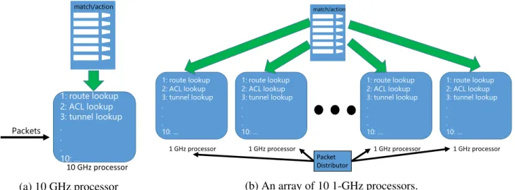
3.3 Strawman 1: a single 10 GHz processor . . . 42
3.4 Strawman 2: an array of processors with shared memory . . . 43
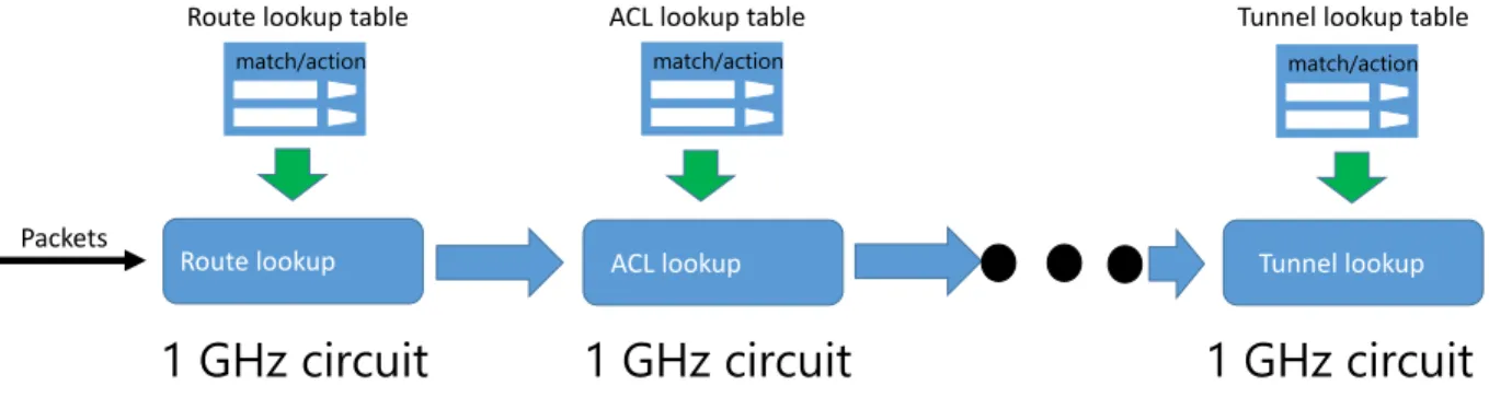
3.5 A pipeline architecture for high-speed routers . . . 44
3.5.1 The internals of a single pipeline stage . . . 44
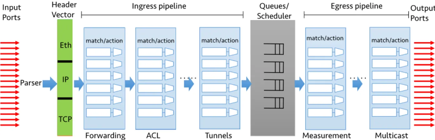
3.5.2 Flexible match-action processing . . . 45
3.6 Using multiple pipelines to scale to higher speeds . . . 46
3.7 Clarifying router terminology . . . 47
3.8 Summary . . . 47
4 Domino: Programming Stateful Data-Plane Algorithms 49 4.1 A machine model for programmable state manipulation on high-speed routers . . . 50
4.1.1 The Banzai machine model . . . 52
4.1.2 Atoms: Banzai’s processing units . . . 52
4.1.3 Constraints for line-rate operation . . . 54
4.1.4 Limitations of Banzai . . . 54
4.2 Packet transactions . . . 54
4.2.1 Domino by example . . . 55
4.2.2 The Domino language . . . 56
4.2.3 Triggering the execution of packet transactions . . . 56
4.2.4 Handling multiple transactions . . . 57
4.3 The Domino compiler . . . 58
4.3.1 Preprocessing . . . 58
4.3.2 Pipelining . . . 60
4.3.3 Code generation . . . 61
4.3.4 Related compiler techniques . . . 62
4.4 Evaluation . . . 63
4.4.1 Expressiveness . . . 64
4.4.3 Compiling Domino algorithms to Banzai machines . . . 66
4.4.4 Generality or future proofness of atoms . . . 68
4.4.5 Lessons for programmable routers . . . 72
4.5 Summary . . . 73
5 PIFOs: Programmable Packet Scheduling 75 5.1 Deconstructing scheduling . . . 76
5.1.1 pFabric . . . 77
5.1.2 Weighted Fair Queueing . . . 77
5.1.3 Traffic shaping . . . 77
5.1.4 Summary . . . 78
5.2 A programming model for packet scheduling . . . 78
5.2.1 Scheduling transactions . . . 79
5.2.2 Scheduling trees . . . 79
5.2.3 Shaping transactions . . . 81
5.3 The expressiveness of PIFOs . . . 83
5.3.1 Least Slack-Time First . . . 83
5.3.2 Stop-and-Go Queueing . . . 84
5.3.3 Minimum rate guarantees . . . 84
5.3.4 Other examples . . . 85
5.3.5 Limitations of the PIFO programming model . . . 86
5.4 Design . . . 87
5.4.1 Scheduling and shaping transactions . . . 88
5.4.2 The PIFO mesh . . . 88
5.4.3 Compiling from a scheduling tree to a PIFO mesh . . . 90
5.4.4 Challenges with shaping transactions . . . 90
5.5 Hardware Implementation . . . 91
5.5.1 Performance requirements for a PIFO block . . . 91
5.5.2 A single PIFO block . . . 92
5.5.3 Interconnecting PIFO blocks . . . 95
5.5.4 Area overhead . . . 95
5.5.5 Additional implementation concerns . . . 97
5.6 Summary . . . 98
6 Marple: Programmable and Scalable Network Measurement 99 6.1 The Marple Query language . . . 102
6.1.1 Packet performance stream . . . 102
6.1.2 Restricting packet performance metadata of interest . . . 103
6.1.3 Computing stateless functions over packets . . . 103
6.1.4 Aggregating statefully over multiple packets . . . 103
6.1.5 Chaining together multiple queries . . . 104
6.1.6 Joining results across queries . . . 105
6.2 Scalable Aggregation at a Router’s Line Rate . . . 106
6.2.1 The associative condition . . . 108
6.2.2 The linear-in-state condition . . . 108
6.2.3 Scalable aggregation functions . . . 109
6.2.4 Handling non-scalable aggregations . . . 110
6.2.5 A unified condition for mergeability . . . 110
6.2.5.1 Notation . . . 110
6.2.5.2 The closure graph . . . 111
6.2.5.3 Proofs of theorems . . . 112
6.2.6 Related work on distributed aggregations . . . 116
6.2.7 Hardware feasibility . . . 117
6.3 Query compiler . . . 118
6.3.1 Network-wide to router-local queries . . . 119
6.3.2 Query AST to pipeline configuration . . . 120
6.3.3 Handling linear-in-state aggregations . . . 121
6.4 Evaluation . . . 124
6.4.1 Hardware compute resources . . . 124
6.4.2 Memory and bandwidth overheads . . . 125
6.4.3 Case study #1: Debugging microbursts . . . 128
6.4.4 Case study #2: Flowlet size distributions . . . 130
6.5 Summary . . . 130
7 Limitations 131 7.1 Limitations common to all three systems . . . 131
7.1.1 Lack of silicon implementations . . . 131
7.1.2 Lack of completeness theorems . . . 132
7.1.3 Lack of a user study . . . 132
7.1.4 Supporting routers with multiple pipelines . . . 132
7.2 Domino limitations . . . 133 7.3 PIFO limitations . . . 134 7.4 Marple limitations . . . 134 8 Conclusion 135 8.1 Broader impact . . . 135 8.2 Future work . . . 136
8.3 Towards a world of programmable networks . . . 138
A The Merge Procedure for Linear-in-state Functions 139 A.1 Single packet history . . . 139
Previously Published Material
Chapter 4 revises a previous publication [187]: Anirudh Sivaraman, Alvin Cheung, Mihai Budiu, Changhoon Kim, Mohammad Alizadeh, Hari Balakrishnan, George Varghese, Nick McKeown, and Steve Licking. Packet Transactions: High-Level Programming for Line-Rate Switches. In SIGCOMM, Florianopolis, Brazil, August 2016.
Chapter 5 combines material from two previous publications [188, 189]:
1. Anirudh Sivaraman, Suvinay Subramanian, Anurag Agrawal, Sharad Chole, Shang-Tse Chuang, Tom Edsall, Mohammad Alizadeh, Sachin Katti, Nick McKeown, and Hari Bal-akrishnan. Towards Programmable Packet Scheduling. In HotNets, Philadelphia, U.S.A, November 2015.
2. Anirudh Sivaraman, Suvinay Subramanian, Mohammad Alizadeh, Sharad Chole, Shang-Tse Chuang, Anurag Agrawal, Hari Balakrishnan, Tom Edsall, Sachin Katti, and Nick McKeown. Programmable Packet Scheduling at Line Rate. In SIGCOMM, Florianopolis, Brazil, August 2016.
Chapter 6 revises a previous publication [166]: Srinivas Narayana, Anirudh Sivaraman, Vikram Nathan, Prateesh Goyal, Venkat Arun, Mohammad Alizadeh, Vimalkumar Jeyakumar, and Changhoon Kim. Language-Directed Hardware Design for Network Performance Monitoring . In SIGCOMM, Los Angeles, U.S.A, August 2017.
Acknowledgments
As a Ph.D. student, I was fortunate to work with two outstanding advisors, Hari Balakrishnan and Mohammad Alizadeh. Each contributed a unique perspective to my research. Hari was the master of the highest-order bit. He taught me to focus on the most important thing at every turn, whether it was an elusive sentence required to finish a paragraph, the key takeaway from a slide, or a single sentence summarizing a paper’s novelty. Hari took me on as his student when my options were limited; this dissertation is my way of repaying that debt. Mohammad taught me to persist until a concept was clear to the point of being obvious. He made me appreciate the peace of mind that comes with mathematical rigor and showed me how to work with hardware engineers. Most importantly, he taught me how to listen and continuously incorporate feedback into my research.
Keith Winstein was a friend and mentor through grad school. He taught me to love clean code, corrected my writing, showed me how to give an engaging talk, and convinced me that it was always possible to program a computer to do your bidding. In April 2013, he wrote a blog post wondering why software-defined networking did not include the data plane. This dissertation is a belated answer to his question.
My thesis committee members, George Varghese and Nick McKeown, helped shape my research taste. George taught me to go beyond the surface in interdisciplinary research. He pushed me to discover precise connections to and differences from adjacent disciplines. Nick suggested that I spend some time interning at Barefoot Networks—an internship that significantly improved my dissertation. He showed me through his own example that it was possible to combine intellectual rigor and practical impact.
As part of my dissertation work, I spent a year interning at Barefoot Networks. It is not often that a fledgling startup gives an intern free rein to pursue open-ended research. My manager, Changhoon Kim, gave me the freedom to go after ideas that I thought were interesting, while ensuring that I was still productive. Mihai Budiu taught me how to engineer a compiler. Anurag Agrawal patiently explained a router’s scheduler to me. In addition, I benefited from conversations with many other engineers and interns at Barefoot, including Antonin, KRam, Ravindra, CK, Pat, Mike, and Naga. This dissertation is the result of joint work with many collaborators: Alvin Cheung, Mihai Budiu, Changhoon Kim, Mohammad Alizadeh, Hari Balakrishnan, George Varghese, Nick McKe-own, Steve Licking, Suvinay Subramanian, Sharad Chole, Shang-Tse Chuang, Anurag Agrawal, Tom Edsall, Sachin Katti, Srinivas Narayana, Vikram Nathan, Prateesh Goyal, Venkat Arun, and Vimalkumar Jeyakumar. The broader P4 community provided an ideal setting for my work, both to get feedback and for translating some of these ideas into practice.
Jonathan, Peter, Hongzi, Pratiksha, Somak, Ameesh, Alvin, Eugene, Swarun, Jason, and Tushar, provided a great reason to come to work, whether to bounce off ideas, get feedback on a talk or paper draft, complain about grad school, get ice cream at Tosci’s, or play an afternoon game of ping-pong. In particular, Ravi has been a great sounding board over the years, tempering my naive optimism with some practical reality checks.
Suvinay and I spent many years in grad school together. I am grateful for our friendship and for his ability to patiently explain hardware to me at all hours of the day and night. As undergrads, Srinivas and I spent many sleepless nights debugging problem sets together. Srinivas started his post doc at MIT just as I was looking around for ideas, allowing us to work together again on a slightly harder problem set: Chapter 6. My friends outside grad school, Raghav, Aakash, Akhil, Raghunandan, Siddharth, and Praneeth, provided me with much-needed breaks from work with the occasional catch ups.
Sheila Marian was a phenomenal admin assistant, assisting with paper work when I was away from MIT, booking travel for me, and ordering cakes for thesis defenses. Janet Fischer at the EECS graduate office patiently extended every Ph.D. deadline. My academic advisor, Piotr Indyk, looked out for me since my first year at MIT, especially when I was switching advisors. Sylvia Hiestand at the MIT ISO got all of my paper work in order during my year away from MIT.
My parents, Rama and Sivaraman, put up with my churlish ways during my time in grad school. I am grateful to them for their patience and for not asking me when I would graduate. My sister, Vibhaa, patiently proofread this dissertation and filed it on my behalf. My grandmother’s utter lack of interest in my research is a much needed breath of fresh air. My in-laws were a steady source of support from afar during my job search. My wife, Tejaswi, went through both the highs and lows of my Ph.D. along with me. I am grateful for her ability to listen carefully, for believing in me for no good reason, and for her honest advice during difficult times.
My late grandfather, Dr. V. Ramamurti, was the reason I embarked on a Ph.D. Throughout high school, he spent an inordinate amount of time patiently teaching me mathematics and physics and indulging my pesky questions. As a faculty member, who also consulted for industry, he taught me not to stray too far from reality when conducting research. I dedicate this dissertation to him.
Chapter 1
Introduction
1.1
Background
Computer networks contain two types of elements: end hosts that generate packets and routers1that forward these packets between the end hosts. Historically, the Internet was architected so that most of the complexity resided in the end hosts, while the routers themselves were simple. According to Clark [95], this architecture was a result of the primary design goal of the Internet: the ability to easily interconnect a wide variety of existing networks (e.g., long-haul networks, local-area networks, satellite networks, and radio networks) through a set of routers between these networks. Quoting Clark, “The Internet architecture achieves this flexibility by making a minimum set of assumptions about the function which the net will provide.”
The minimum functionality assumed of and provided by the network’s routers was best-effort and unreliable packet forwarding. Notably absent from a router’s feature set were reliable packet delivery, packet prioritization, monitoring features to attribute a router’s resource usage to specific end hosts, and security features to detect network breaches. As a result, the early routers were singularly dedicated to packet forwarding. A focus on packet forwarding alone made it simpler to design high-speed routers. It also helped broaden the Internet’s reach by interconnecting existing networks with minimum friction. But, it sidelined other goals [95] such as network performance, security, and monitoring.
Today, four decades after ideas underlying the Internet were first published [90], it is clear that routers need to do much more than packet forwarding for at least two reasons. First, once the basic goal of interconnecting different networks is achieved, other goals like performance, security, and monitoring rise in prominence. Second, many large-scale private networks (e.g., datacenters, private wide-area networks, and enterprise networks) do not need to concern themselves with interconnecting diverse networks as the Internet had to. Such private networks can expect more from the network. As a result, a typical router today implements many features beyond packet forwarding, pertaining to security (e.g., access control), monitoring (e.g., counting the number of packets belonging to each flow), and performance (e.g., priority queues).
While a router’s feature set has grown steadily with time, there’s little consensus between
1980s 1990s 2000s 2010s WFQ VirtualClock CSFQ STFQ Bloom Filters DRR RED AVQ XCP RCP CoDel DeTail DCTCP HULL SRPT PIE
IntServ DiffServ ECN
Flowlets
PDQ
HPFQ FCP
Heavy Hitters
Figure 1-1: Timeline of prominent router algorithms since the 1980s. Only the ones shaded in blue are available on the fastest routers today.
network operators and router vendors on a router’s feature set. Inevitably, there are network operators whose needs fall outside their router’s feature set. But, because today’s fastest routers are built out of specialized forwarding hardware, they are largely fixed-function2devices, i.e., their functionality cannot be changed once the router has been built. In such cases, the operator has no alternative but to wait 2–3 years for the next generation of the router hardware. This is best illustrated by the lag time between the standardization and availability of new overlay protocols [34].
As a result, the rate of innovation in new router algorithms is outstripping our ability to get these algorithms into today’s fastest routers, i.e., routers with between 10 and 100 ports, each running at between 10 and 100 Gbit/s. Figure 1-1 shows a timeline of prominent router algorithms that have been developed since the 1980s. Of these, only a handful are available in the fastest routers today because there is no way to program a new router algorithm on these routers.
Against this backdrop, if an operator wants to introduce new network functionality, what are her choices? One is to give up on changing routers altogether and make all the required changes at the end hosts. Relying solely on the end hosts, however, results in cumbersome or suboptimal solutions. As a first example, imagine measuring the queueing latency at a particular hop in the network. One could do this by collecting end-to-end ping measurements between a variety of vantage points and then fusing these measurements together to estimate per-hop queueing latency—a process commonly called network tomography. Not only is this indirect, it is also inaccurate relatively to directly instrumenting the router at that hop to measure its own queueing latency. As a second example, consider the problem of congestion control, which divides up a network’s capacity fairly among competing users. There are many in-network solutions to congestion control [138, 194], which outperform the end-host-only approaches to congestion control used today [122, 197]. However, there is no way to deploy these in-network solutions using a fixed-function router today.
Another alternative is to use a software router: a catch-all term for a router built on top of some programmable substrate, such as a general-purpose CPU [143, 103], a network processor,3a
graphics processing unit (GPU) [123], or a field-programmable gate array (FPGA) [215]. Figure 1-2 tracks the evolution of aggregate capacity of software routers and compares them to the fastest routers known at any point in time. The figure shows two trends. First, until the mid 1990s, software routers were in fact the fastest routers; the early routers [126] were minicomputers loaded with forwarding software. Second, since the mid 1990s, growing demands for higher link speeds, fueled
2The term fixed-function was first used to describe graphics processing units (GPUs) with limited or no
programma-bility [16]. We use it in an analogous sense here.
Catalyst Broadcom5670 Scorpion TridentTridentII Tomahawk IMP MIT CGW Fuzzball Proteon SNAP (Active Networks) Click (CPU) IXP 2400 (NPU) RouteBricks (multi-core) PacketShader (GPU) NetFPGA-SUME (FPGA) 0.0004 0.004 0.04 0.4 4 40 400 4000 1969 1982 1983 1985 1999 2000 2002 2004 2007 2009 2010 2012 2014 Gbit/s (log scale) Year Fastest router Software router
Figure 1-2: Aggregate capacity of software routers since the first router on the ARPANET in 1969 [126]. Until the mid 1990s, software routers were sufficient. Since then, however, the fastest routers have largely been fixed-function devices, built out of dedicated non-programmable hardware, which gives these routers a 10–100x performance improvement relative to the best software routers.
by the Internet’s growth, have meant that the fastest routers are now built out of dedicated hardware. Hardware specialization gives today’s fastest routers a 10–100 × performance improvement relative to the fastest software routers. This performance improvement is the result of fully exploiting the abundant parallelism available in packet processing. First, data parallelism, the ability to simultaneously process either different parts of the same packet or packets belonging to different ports. Second, pipeline parallelism, the ability to simultaneously perform different operations on different packets. But, hardware specialization carries a cost: because routers are built out of specialized hardware, they are fixed-function devices that can not be programmed in the field.
Recent work in software-defined networking [108] (SDN) and programmable router chips [86, 60, 25] has endowed fast routers with limited flexibility. SDN allows operators to program the network’s control plane, which is the part of the network that computes a network’s routing tables. SDN does this by moving route computations out of the routers and on to a logically centralized programmable server running on a CPU.
Programmable router chips allow operators to program parts of the data plane: the part of the network that forwards packets based on the routing tables. For instance, these chips allow an operator to program the router’s parser to recognize new packet headers, such as a new overlay format [34]. They also allow the operator to program packet header transformations (e.g., decrementing the IP TTL field) so long as these transformations do not modify router state.
However, both SDN and programmable router chips are still insufficient to express the grayed-out algorithms shown in Figure 1-1 because (1) these algorithms programmatically manipulate router state and (2) they require flexibility in packet scheduling. State modification on routers and the router’s scheduler are largely ignored by both SDN and programmable router chips.
1.2
Primary contributions
This dissertation considers the problem of designing routers that approach the speeds of today’s fastest fixed-function routers, while also being programmable. My thesis is that it is possible to design router hardware that is both fast and programmable, if we restrict ourselves to program-ming specific classes of router functionality. It is this specificity that allows us to resolve the programmability-performance tension; indeed, our designs provide a much more restricted form of programmability than a Turing-complete processor.
The challenge here is to pick classes of router functionality that are simultaneously (1) practically useful to network operators, (2) broad enough to cover a range of current and future use cases within that class, and yet (3) narrowly focused enough to permit a high-speed hardware implementation. We will describe high-speed programmable hardware primitives and their corresponding programming models in software for three classes of router functionality: stateful data-plane algorithms, packet scheduling, and scalable network measurement. Table 1.1 summarizes our contributions. §1.3, §1.4, and §1.5 expand on each of the three contributions.
1.2.1
Evaluation metrics
The goal of this dissertation is to design fast and programmable routers. Accordingly, we measure each of our three systems on two attributes, performance and programmability, as described below.
The traditional approach to evaluating performance of a software system is to measure the system’s throughput on some workloads. This approach does not apply to evaluating hardware designs, which are built for a specific clock rate or throughput. Hardware designs provide this clock rate or throughput even under worst-case conditions, regardless of the workload presented to them.
To provide worst-case guarantees, hardware designs exploit spatial parallelism—by chaining together computations in a pipeline (pipeline parallelism) and simultaneously performing multiple operations within a pipeline stage (data parallelism). Put differently, hardware designs spend circuit area in return for deterministic high performance. The question then is whether these designs consume a large amount of area to provide such performance guarantees and whether they can provide acceptable performance, as measured by the design’s clock rate.
Hence, to evaluate performance, we estimate if the hardware components of our systems can run at a high clock rate while not taking up too much gate and wire area. To do so, we code any new hardware components as programs in the Verilog hardware description language. We then pass this Verilog program to a logic synthesis tool [12, 6] that produces a gate-level implementation from Verilog programs. The synthesis tool also reports whether the resulting implementation meets timing at a given clock frequency and the area taken up by the gates in the implementation.4 When we say a hardware design is feasible, we mean that it meets timing at a high clock frequency (1 GHz in this dissertation) and its gate area is modest relative to the area of a router chip (200 mm2in
this dissertation based on the minimum area estimates provided by Gibb et al. [115]).
4A full hardware implementation also requires a place-and-route [41] step after logic synthesis to physically place
these gates and route wires between them. This increases the area of designs, especially if the design is dominated by wires, as is the case with crossbars. Because our designs are dominated by gates, not wires, we do not perform this place-and-route step when estimating area.
Stateful data-plane algorithms (Chapter 4)
Examples: In-network congestion control (e.g., XCP [138] and RCP [194]), active queue management (e.g., RED [111], BLUE [109], and CoDel [168])
Technical challenge: How do we allow programmable router state modification at the router’s line rate, when a new packet can be received as often as every nanosecond?
Programming model: Packet transactions (§4.2) Hardware primitive: Atoms (§4.1)
Key finding: A small set of atoms (Table 4.4) is simultaneously (1) expressive enough to serve as the instruction set for many stateful algorithms (Table 4.5) and (2) feasible in high-speed hardware (§4.4). Further, we find that these atoms can support several new use cases that were unanticipated at the time the atoms were designed (Table 4.6).
Scheduling algorithms (Chapter 5)
Examples: Weighted Fair Queueing [99] and priority scheduling [182]
Technical challenge: Can we find an abstraction that unifies many disparate scheduling algorithms? Programming model: Scheduling trees (§5.2)
Hardware primitive: A priority queue data structure called a Push In First Out Queue (PIFO) (§5.4)
Key finding: A priority queue of packets with a program to set each packet’s priority can express many scheduling algorithms (§5.3) and is feasible in high-speed hardware (§5.5).
Scalable per-flow statistics (Chapter 6)
Examples: Per-flow measurements of moving averages, counters, and loss rates
Technical challenge: Can we allow programmers to flexibly define the per-flow statistics they want to measure and also scale these measurements to a large number of flows?
Programming model: Performance queries (§6.1)
Hardware primitive: Programmable hardware key-value store. Keys correspond to flows and values to statistics. (§6.2)
Key finding: A class of statistics measurements, which we call the linear-in-state class (§6.2.2), can be scaled to a large number of flows without losing accuracy. This class covers many practically useful statistics such as counters, moving average filters, and conditional counters (§6.4).
To evaluate if our systems are programmable, we evaluate the expressiveness of the program-ming models in each of our systems. If we are able to express a diversity of algorithms using the programming models, we say that the programming model is expressive. Our approach to expressiveness is empirical: beyond specific examples, we do not have theoretical characterizations of the set of programs that can or cannot be programmed using our programming models (§7.1.2). In addition, to assess the correctness of our designs, we built a C++ simulator of a programmable router that models the behavior of the essential computational elements of a programmable router at the level of individual clock cycles (§4.1).
1.3
Stateful data-plane algorithms
In Chapter 4, we consider the problem of programming stateful data-plane algorithms at high packet processing rates. These are algorithms that operate on a sequence of packets in a streaming manner, doing a bounded amount of work per packet and manipulating a bounded amount of router state in the process. They include algorithms for managing the router’s buffer (e.g., RED [111] and BLUE [109]), load balancing (e.g., CONGA [65] and flowlet switching [186]), and in-network congestion control (e.g., XCP [138] and RCP [194]).
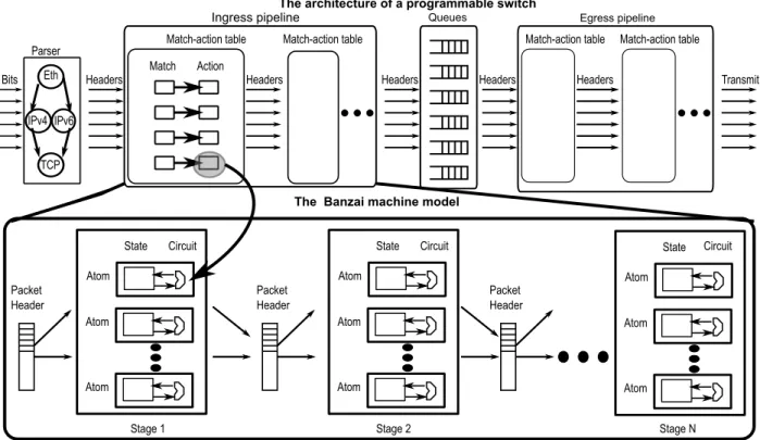
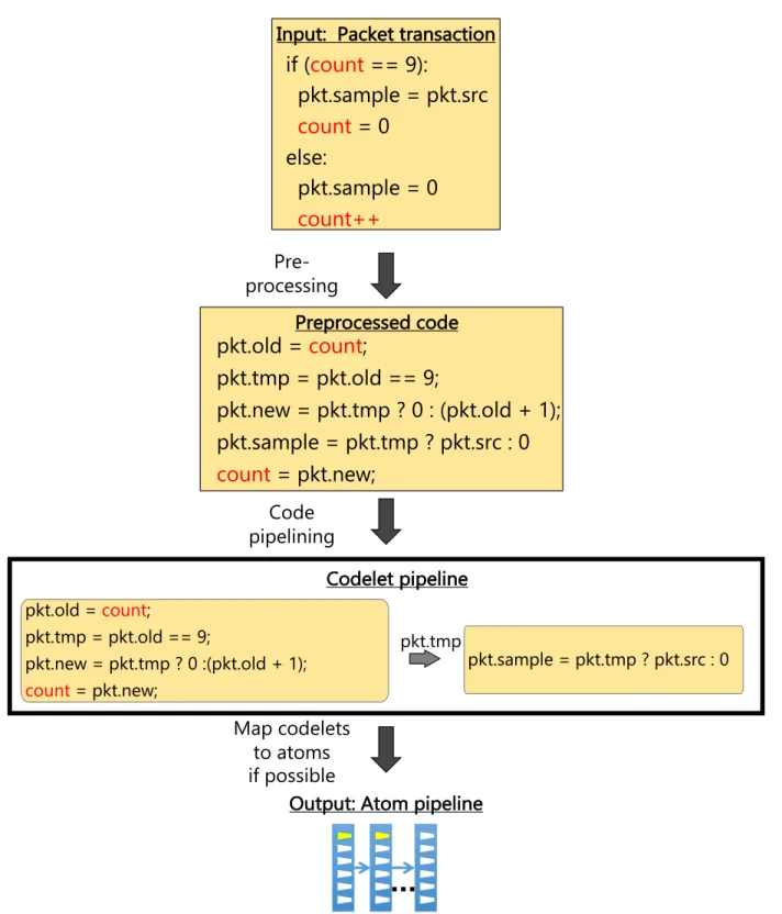
High-speed data-plane programming on routers poses two challenges: (1) what hardware instructions are required to support programmable state modification at high speeds, and (2) what is the right programming model? To address these challenges, we develop a system for data-plane programming, Domino, which contains three main components: an instruction set (atoms), a programming model (packet transactions), and a compiler from packet transactions to atoms.
1.3.1
Atoms: Hardware for high-speed state manipulation
Atomscapture a router’s instruction set. They specify atomic units of packet processing provided by the router hardware, e.g., an atomic counter or an atomic test-and-set. Figure 1-3 shows an example atom. Atoms are atomic in the sense that if some state is updated by an atom as part of processing a packet, the next packet arriving at that atom will see the updated value of that state. The processing within atoms is constrained to meet the atomicity requirement. We enforce this constraint when designing atoms in hardware by ensuring that the input-to-output latency of the atom’s digital circuit is under a clock cycle. This guarantees that any state updated by the atom has been updated to its correct value in time for the next packet arriving at the atom a clock cycle later.5
1.3.2
Packet transactions: A programming model for stateful algorithms
Packet transactionsprovide a programming model for data-plane algorithms. A packet transaction is an atomic and isolated block of code capturing an algorithm’s logic written in a domain-specific language (DSL) called Domino. Figure 1-4 shows an example packet transaction. Packet trans-actions provide programmers with the illusion that the transaction’s body executes serially from
actio
n unit
X const Add Add 2-to-1 Mux X choice pkt.f 1 cycle input-output latencyFigure 1-3: An atom that either adds either a constant or a packet field to a piece of state x and writes it back to x.
if (
count
== 9):
pkt.sample = pkt.src
count
= 0
else:
pkt.sample = 0
count++
Figure 1-4: A packet transaction that samples the source IP address of every 10th packet. State variables (count) are in red.
start to finish on each packet, in the order in which packets arrive at the router. Conceptually, when programming with packet transactions, there is no overlap in packet processing across packets—akin to an infinitely fast single-threaded processor carrying out packet processing on each packet. Packet transactions are expressive and capture many important data-plane algorithms. Further, their serial semantics shield programmers from the router’s data and pipeline parallelism.
1.3.3
Compiling from packet transactions to atoms
The Domino compiler compiles packet transactions written in the Domino DSL to a pipeline of atoms provided by the router. It rejects the code if the router’s atoms cannot support the packet transaction. The compiler bridges the gap between the serial single-threaded execution model seen by the programmer and the data-parallel and pipeline-parallel execution model of the router.
The compiler has three passes (Figure 1-5). First (§4.3.1), it preprocesses the code to make it easier to infer dependencies between packet-processing operations. Second (§4.3.2), the compiler transforms the preprocessed, but still serial, packet transaction into a parallel pipeline of codelets. When pipelining, the compiler maintains the following invariant: if each codelet executes atomically and passes off its results (e.g., pkt.tmp in Figure 1-5) to the next codelet, the behavior will be indistinguishable from the packet transaction itself executing atomically on each packet. Third (§4.3.3), the compiler maps each codelet one-to-one to an atom provided by the underlying router, rejecting the code if the codelet cannot be supported by an atom.
The compiler provides an all-or-nothing guarantee: if the compiler compiles a program, the program will run at the line rate of the router.6 All other programs that cannot run at the router’s
6We use the term line rate in this dissertation to mean both the maximum bit/packet rate of a particular router
port/line (e.g., 10 Gbit/s) and the maximum aggregate bit/packet rate of a router: the product of the per-port line rate and the number of ports (e.g., 64×10 Gbit/s = 640 Gbit/s). It should be clear from the context which interpretation of line rate we are referring to.
Code pipelining
Map codelets to atoms if possible
Output: Atom pipeline Pre-processing
pkt.old =
count
;
pkt.tmp = pkt.old == 9;
pkt.new = pkt.tmp ? 0 : (pkt.old + 1);
pkt.sample = pkt.tmp ? pkt.src : 0
count
= pkt.new;
Preprocessed codeif (
count
== 9):
pkt.sample = pkt.src
count
= 0
else:
pkt.sample = 0
count++
Input: Packet transaction
Codelet pipeline pkt.old = count; pkt.tmp = pkt.old == 9; pkt.new = pkt.tmp ? 0 :(pkt.old + 1); count= pkt.new; pkt.sample = pkt.tmp ? pkt.src : 0 pkt.tmp
Figure 1-5: The three passes of Domino’s compiler shown on the packet transaction from Figure 1-4.
line rate will be rejected. A program may be rejected either because the router’s atoms are not expressive enough for the program’s operations or there aren’t enough atoms for all operations
Atom Algorithm as a packet transaction Domino Compiler Algorithm doesn’t compile? Modify number of atoms or type of atom Algorithm compiles? Move on to another algorithm
Figure 1-6: Iterative atom design process
in the program. A conventional compiler for a general-purpose CPU compiles all programs, but a program’s run-time performance depends on its complexity. In Domino, only programs that are simple enough to run at the router’s line rate will be compiled, obviating the need for any performance profiling.
1.3.4
Evaluation
Developing atoms for a router is a chicken-and-egg problem. A router’s atoms determine what algorithms the router can support, while the algorithms determine what atoms are required in the first place. Designing the right atoms is especially important for a programmable router because, in contrast to a general-purpose CPU, there is no way to “emulate” functionality in software when hardware support is not available: recall that if an atom does not exist to support a program’s operations, the program will be rejected.
To develop atoms, we use the Domino compiler to experiment with different atoms and iteratively modify the atoms until they support enough algorithms (Figure 1-6). Using this process, we developed seven atoms of increasing complexity (Table 4.4) that allow us to progressively program more and more algorithms from Figure 1-1. For instance, measurement using Bloom filters only requires simple read and write operations on state. On the other hand, heavy-hitter detection [209] uses a count-min sketch [96] that relies on an atomic counter. Finally, algorithms like flowlet switching [186] require conditional writes to a state variable.
After freezing the design of these atoms, we found that our atoms could express several new use cases that were unanticipated when the atoms were designed (Table 4.6). This provides us with some evidence that these atoms are indeed programmable and can generalize to new algorithms beyond the initial algorithms that influenced their design in the first place.
1.4
Programmable packet scheduling
Packet scheduling is an important determinant of network performance. The choice of scheduling algorithm is tied to a network’s performance goals. For instance, an algorithm that divides link
capacity fairly is ideal in a multi-tenant setting [99], while the shortest remaining processing time algorithm is ideal for a single tenant who desires low flow completion time [68]. Today’s routers provide a fixed set of scheduling algorithms (e.g., priority queues, Deficit Round Robin [185], and rate limiting [58]). While configuration settings on these scheduling algorithms can be tweaked, there is no way for an operator to program a new scheduling algorithm that is tailored to their needs. Routers lack programmable scheduling because there is no single abstraction to express many scheduling algorithms [99, 182, 179, 68, 149] that appear so different at first brush. This lack of a single unifying abstraction is not merely an academic concern. It has practical consequences: in the absence of a single abstraction that can then be hardened in hardware, we are left with using a general-purpose substrate such as a CPU to program scheduling. As we mentioned earlier, this can hurt performance substantially.
Push In First Out Queues (PIFOs) (Chapter 5) provide such an abstraction.7 They exploit our
observation that in many practical schedulers the relative order of packets that are already buffered does not change in response to new packet arrivals (§5.1). Hence, when a packet arrives, it can be pushed into the right location based on a packet priority (push in), but packets are always dequeued from the head (first out). A PIFO is simply a priority queue of packets with a small program to assign each packet its priority.8 Yet, by flexibly programming a packet’s priority assignment, a
network operator can use PIFOs to program a variety of previously proposed scheduling algorithms.
1.4.1
Programming model for packet scheduling
Our programming model for scheduling couples a PIFO with a program to determine a packet’s rankin the PIFO. This rank can denote the packet’s scheduling order (for work-conserving algo-rithms such as Weighted Fair Queueing [99]) or absolute wall-clock departure time (for non-work-conserving algorithms such as traffic shaping [58]). This program is written as a packet transaction, introduced earlier. Depending on whether the program determines the scheduling order or time, the program is called either a scheduling transaction or a shaping transaction respectively.
A single PIFO coupled with a scheduling or shaping transaction can express many classical scheduling algorithms, e.g., Weighted Fair Queueing (Figure 1-7a) and Token Bucket Shaping (Figure 1-7b). But, a single PIFO is still restricted to scheduling algorithms with the property that the relative order of packets that are already buffered does not change in response to new packet arrivals. A canonical class of scheduling algorithms that violate this relative order property is the class of hierarchical scheduling algorithms. A well-known example of this class is Hierarchical Packet Fair Queueing (HPFQ) [76]. HPFQ first divides up the link’s capacity fairly among classes, and then when each class is scheduled, divides up the class’s transmission opportunities fairly among its constituent flows. It can be thought of a recursive version of fair queueing.
To support hierarchical scheduling, we extend our programming model from a single PIFO to a tree of PIFOs. We also allow an entry in a PIFO to be either a packet or a reference to another PIFO.
7PIFOs were used as a theoretical construct to establish the equivalence of combined input-output queued routers
and output-queued routers [94]. We show here that they can be used practically for programmable packet scheduling.
8We use the term PIFO instead of priority queue because, within the context of networking, priority queues typically
refer to an implementation of work-conserving priority scheduling. PIFOs can be used for both work-conserving and non-work-conserving algorithms (§5.3).
1 f = flow(p) # compute flow from packet p 2 if f in last_finish:
3 p.start = max(virtual_time, last_finish[f]) 4 else: # p is first packet in f
5 p.start = virtual_time
6 last_finish[f] = p.start + p.length/f.weight 7 p.rank = p.start
(a) Scheduling transaction for the Start-Time Fair Queueing implementation [118] of Weighted Fair Queueing.
1 tokens = tokens + r * (now - last_time) 2 if (tokens > B):
3 tokens = B
4 if (p.length <= tokens): 5 p.send_time = now 6 else:
7 p.send_time = now + (p.length - tokens) / r 8 tokens = tokens - p.length
9 last_time = now 10 p.rank = p.send_time
(b) Shaping transaction for Token Bucket Shaping. Figure 1-7: Examples of scheduling and shaping transactions. p.xrefers to a packet fieldxin packet p. yrefers to a state variable that is persisted on the router across packets, e.g.,last_finishand virtual_timein this snippet.p.rankdenotes the packet’s computed rank.
Left
Right
root
True,
WFQ_Root
p.class == Left,
WFQ_Left
p.class == Right,
WFQ_Right
Figure 1-8: Scheduling tree for HPFQ. The scheduling transactions WFQ_Root, WFQ_Left, and WFQ_Right are similar to Figure 1-7a and differ only in how the flow is computed from the packet. This tree has no shaping transaction.
More formally, a node in a scheduling tree (Figure 1-8) has three attributes: (1) a predicate that determines which packets are handled by that node, (2) a scheduling transaction that determines a packet’s rank in a scheduling PIFO attached to that node, and (3) an optional shaping transaction that determines a packet’s rank in an optional shaping PIFO attached to that node. The shaping transaction is optional because it is only relevant to non-work-conserving schedulers. It can be disregarded entirely for work-conserving schedulers.
We now explain the semantics of a scheduling tree during dequeues and enqueues. During a dequeue, we walk the scheduling tree starting from the root. We dequeue the scheduling PIFO at the root, resulting in either a reference to another scheduling PIFO or a packet. If the result is a packet, we are done, and we transmit the packet. If not, we continue recursively, dequeueing from the scheduling PIFO that is pointed to until we find a packet.
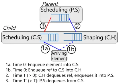
When a packet is enqueued, we walk the tree from the leaf whose predicate captures the packet to the root. Along this leaf-to-root path, we execute scheduling and (optionally) shaping transactions attached to the path’s nodes. Figure 1-9 illustrates the timing of various operations related to a node’s scheduling and a shaping PIFO. A node’s scheduling transaction inserts either a packet or a
Parent
Child
1a
2
3
1a. Time 0: Enqueue element into C.S. 1b. Time 0: Enqueue ref to C.S into C.H.
2. Time T (> 0): C.H dequeues ref, enqueues it into P.S. 3. Time T’ (> T): P.S dequeues from C.S.
Shaping (C.H)
Scheduling (C.S)
Scheduling (P.S)
1b
Arriving ElementFigure 1-9: Child’s shaping transaction (1b) defers enqueue into Parent’s scheduling PIFO (2) until time T. Blue arrows show enqueue paths. Red arrows show dequeue paths.
PIFO reference into the node’s scheduling PIFO. A node’s shaping transaction inserts a reference 𝑅 to the node’s scheduling PIFO in the node’s shaping PIFO. Once the shaping transaction has executed, execution of transactions for this packet is temporarily suspended. When the reference 𝑅 is dequeued from the shaping PIFO, it is enqueued into the node’s parent’s scheduling PIFO using the parent’s scheduling transaction and the rest of the leaf-to-root path is resumed. The shaping PIFO thus provides an optional mechanism for a node to defer enqueues into its parent’s scheduling PIFO, which is useful when combining hierarchical scheduling with traffic shaping (Figure 5-4 in Chapter 5 shows an example.).
1.4.2
Expressiveness of our programming model
The PIFO-based programming model unifies several scheduling algorithms and allows us to program a wide variety of scheduling algorithms using the single PIFO primitive, e.g., Weighted Fair Queueing [99], Token Bucket Shaping [58], Hierarchical Packet Fair Queueing [76], Least-Slack Time-First [149], the Rate-Controlled Service Disciplines [213], and fine-grained priority scheduling (e.g., Shortest Job First).
1.4.3
Hardware for programmable scheduling
We designed high-speed hardware to support a PIFO-based programming model. When designing hardware for PIFOs, we set out to meet performance targets that are typical for a single-chip shared-memory router today. These are routers that are built out of a single chip,9and whose packet
buffer and scheduling logic is shared across all ports. Sharing the packet buffer and scheduling logic reduces the memory and digital logic cost associated with packet scheduling.
For concreteness, we picked a target clock frequency of 1 GHz to reflect the requirement of performing one enqueue and one dequeue every nanosecond, typical of high-speed routers today [86]. We targeted a packet buffer of size 12 MByte based on the buffer size of the Broadcom Trident II [40], a commercial single-chip shared-memory router. With a cell size of 200 bytes,10a 12 MByte buffer can support up to 60000 packets in the worst case.
Hence we need a PIFO that can support up to 60K packets. A naive way to implement a 60K-entry PIFO is to use a flat sorted array of 60K elements and insert an incoming element into this array in a manner reminiscent of insertion sort. Concretely, an incoming element’s rank would be compared in parallel to the ranks of all 60K elements. This would produce a bitmask denoting which elements were greater than or lesser than the incoming element. Because the array is always sorted, the bitmask would have a single 0-to-1 transition. The position of this 0-to-1 transition could be detected using a priority encoder. Finally, the new element could be inserted into this position. However, the difficulty with this approach of using a flat sorted array is that it is hard to lay out 60K parallel comparators, one for each element in the PIFO.
Instead, we exploit the observation that in most practical scheduling algorithms, scheduling is performed across flows and not individual packets. This is because, in most schedulers, packet ranks increase monotonically across consecutive packets within a flow. This ensures that packets within a flow are transmitted in the order in which they arrive, thereby preventing packet reordering within a flow.
Because ranks increase monotonically within a flow, we only need to look at the first packet of each flow to determine which packet to dequeue next. This reduces the number of elements that need to be sorted from 60K packets in the naive implementation to around 1K flows in the smarter implementation. We picked this 1K number with reference to the Broadcom Trident II that supports ~10 queues on each of its ~100 ports.
We find that transistor technology has evolved to the point where it is relatively cheap to build a sorted array of 1K flows, where a flow can be enqueued into or dequeued from the array every nanosecond. In a recent industry-standard 16 nm technology node, a hardware design for a programmable 5-level hierarchical scheduler costs less than 4% additional chip area relative to a 200 mm2baseline router chip [116].
1.5
Programmable and scalable network measurement
Chapter 6 considers the problem of programmable and scalable network measurement. Concretely, can we allow network operators to flexibly specify the per-flow statistics they want to measure (e.g., a moving average over queueing latencies or a count of packets or bytes) at the flow granularity they desire (e.g., at the 5-tuple level or at the level of each distinct destination IP address)? Current router solutions for measurement [8, 11] fix either the statistics that can be measured or the granularity at which the statistics can be measured. The challenge here is to provide a set of measurement primitives that can cover a range of statistics while also scaling to a large number of flows, because the granularity of a flow can be as fine-grained as the 5-tuple.
result = filter(pktstream, qid == Q && tout - tin > 1ms)
// Filter out packets whose queueing delay at queue Q exceeds one ms. result = map(pktstream, [tin/epoch_size], [epoch])
// Round off packet time stamps to the nearest epoch of size epoch_size. def count([c], []):
c = c + 1
result = groupby(pktstream, [5tuple], count)
// Partition packets by 5-tuple and count the number of packets in each 5-tuple. Figure 1-10: Three example Marple queries. pktstreamrefers to the original packet performance stream with one tuple for each packet seen in the network.
1.5.1
Programming model
To allow network operators to express a wide range of performance measurement questions, we provide them with the abstraction of a single performance packet stream for the entire network. Conceptually, the performance packet stream is a stream of tuples, one for each packet, containing information identifying the packet (source and destination address and ports) and its performance information (the timestamp at which the packet was enqueued/dequeued at each network queue).
Network operators can write queries that operate on this performance packet stream using a query language called Marple. Marple has functional constructs like map,filter, andgroupby similar to functional APIs in programming languages like Python, Java, Scala, and Haskell. Figure 1-10 shows some example queries in Marple. These constructs take a stream of tuples as input and return an output stream of tuples. Because all constructs produce and consume streams, Marple queries can be easily composed.
The output stream either transforms each tuple in the input stream (map), drops certain tuples from the input stream based on a predicate (filter), or partitions the input stream into substreams and then aggregates the tuples within each substream based on a user-defined aggregation function (groupby). Marple’s use of user-defined aggregation functions differentiates its groupby construct from the groupby construct supported by classical query languages like SQL. SQL only supports specific order-independent aggregation functions like counts and averages. Unlike Marple, SQL does not allow general, user-defined, and potentially order-dependent aggregation functions.
1.5.2
Hardware for programmable network measurement
A naive implementation of performance queries would stream relevant performance information for every packet to a centralized collection server, which would execute the performance query on the incoming packet stream. However, this would require enormous computational capacity on the server and a separate measurement network just to stream per-packet information to the server. For instance, modern stream processing systems support a throughput of ~100K–1M operations per second per core [4, 21, 125, 2, 48], but processing every single packet from a single 1 Tbit/s
router requires around ~100M operations per second even for relatively large 10000 bit packets. Instead, we use programmable routers as first-class citizens to perform early filtering, aggregation, and packet transformations. The net effect is a substantial reduction in the amount of data sent out to and processed by the collection server.
Many of Marple’s constructs (e.g.,mapandfilter) are stateless in the sense that they do not need to maintain any router state. For instance, amapquery could take an input packet stream, round off the enqueue timestamp of each packet in the stream to the nearest millisecond, and return the result as a new stream. This query is stateless because it can operate independently on each packet without maintaining any state on the router that persists between packets. Supporting stateless queries is relatively straightforward. Emerging programmable router chips [86, 60, 25, 3] already provide an instruction set that performs stateless transformations on packet headers. We leverage this instruction set as is to execute stateless queries because a packet-processing pipeline naturally fits the streaming model of our queries.
On the other hand, the groupbyquery is stateful. To see why, consider agroupy query that (1) partitions the packet stream into substreams based on the 5-tuple and (2) counts the number of packets within each substream. This query is stateful because it needs to maintain a dictionary mapping each 5-tuple to its count as part of the persistent router state. To implement thegroubpy query, this dictionary is updated by incrementing some 5-tuple’s counter on each packet. To support Marple’sgroupby, we design a programmable key-value store in hardware. The keys represent the flows and the values represent the state being aggregated according to the aggregation function as packets are processed. In the example above, the key would be a 5-tuple and the value would be a count of packets belonging to that 5-tuple.
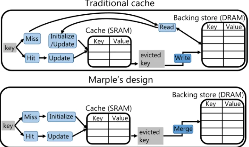
This key-value store has two requirements that are at odds with each other: it needs to be fast to process packets at the router’s line rate (a packet every nanosecond), and it needs to be large to store a large number of flows. Static random-access memory (SRAM) can be accessed once every nanosecond, but has low memory density and can only fit a small number of flows. On the other hand, dynamic random-access memory (DRAM) has much better density allowing it to support many more flows, but can be accessed only once every ten nanoseconds or so.
We use caching to address both requirements: a fast SRAM cache stores the currently active flows, while a backing store in DRAM handles evictions from the cache. However, cache misses in traditional processor designs lead to unpredictable memory access latencies while the data is being fetched from the main memory. A processor handles this by occasionally stalling its pipeline to handle a cache miss. But stalling a router pipeline prevents us from providing the deterministic latency guarantees that routers are known and benchmarked for.
Instead, as Figure 1-11 shows, we treat a cache miss as the arrival of a packet from a new flow and initialize the cache entry as though we have just started aggregating packets from a new flow. When this cache entry is eventually evicted, we merge it against the old value for that entry in the backing store. The merge operation requires reading and writing from DRAM, which does incur unpredictable access latencies. But, it happens off the critical path during evictions alone. Importantly, it does not affect the critical path of packet processing in the router’s chip.
What exactly does this merge operation look like? As a simple example, if the value in the key-value store was a counter; the merge operation would then simply add up the old and new
Key Value Key Value key Merge evicted key Key Value Key Value
Backing store (DRAM)
Write evicted key
Cache (SRAM)
Cache (SRAM)
Backing store (DRAM)
Hit Miss Update Initialize key Hit Miss Update Initialize /Update Read Traditional cache Marple’s design
Figure 1-11: Marple’s key-value store vs. a traditional cache
counts. But is it always possible to merge an aggregation function accurately i.e., the value after the merge should be the same as the value that would be obtained in an ideal system with an infinitely large cache that needs no merging?
We can prove (§6.2.5.3) that there are aggregation functions for which it is not possible to merge efficiently without losing accuracy. However, we formally characterize a class of aggregation functions for which such merging is possible without losing accuracy. We call this class the class the linear-in-state class because aggregation functions in this class take the following form:
𝑆 = 𝐴(𝑝) * 𝑆 + 𝐵(𝑝) (1.1)
Here 𝑆 is the state/value that is being updated by the aggregation function, while 𝐴 and 𝐵 are functions of a bounded number of packets into the past including the current one. The linear-in-state class captures a variety of aggregation functions including counters, predicated counters, moving average filters, and arbitrary functions on sliding windows.
1.5.3
Evaluation
We evaluate Marple’s expressive power by using it to express several diverse performance queries, e.g.,tracking the loss rate on a per-flow basis, measuring the extent of reordering in a TCP flow, measuring a moving average of queueing latencies on a per-flow basis, and detecting the presence of TCP incast [201].
Our Marple compiler compiles queries to two different targets: an atom pipeline to determine the hardware feasibility of Marple queries and a P4-based software router [37] for end-to-end case studies of Marple in Mininet [148]. We find that Marple queries occupy a small fraction of the router’s computational and memory resources. Computationally, queries require a small number of atoms. Memory-wise, the programmable key-value store requires an SRAM cache that occupies a modest amount of additional chip area. Our Mininet experiments show that Marple can be used to iteratively troubleshoot problems such as occasional latency spikes that occur because of bursty
background traffic.
We determine the eviction rate from the SRAM cache using a trace-driven simulation on publicly available packet traces from CAIDA [54, 53] and a university datacenter [78]. For a 64 Mbit on-chip cache, which occupies about 10% of the area of a 64×10-Gbit/s router chip, we estimate that the cache eviction rate from a single top-of-rack router can be handled by a single 8-core server running Redis [43]. Relative to a strawman that sends every packet to the collection server (i.e., a 100% eviction rate), the on-chip cache results in a reduction in eviction rate of 34–81x (Figure 6-8).
1.6
Lessons learned
We conclude this chapter by distilling some general lessons for designing fast and programmable routers in the future that go beyond the specific contributions of each of the three systems.
1.6.1
The power of specialization
The most important lesson here is the power of specialization: the idea of targeting hardware and software to specific classes of router functionality. The three systems in the dissertation demonstrate how narrowing our focus to specific router functionality allows us to resolve the performance-programmability tradeoff that has affected software routers so far. Put differently, it allows us to get the best of both worlds, but for restricted classes of router functionality.
More formally, the three systems are specialized in the sense that they are not Turing-complete: they cannot simulate a Turing machine, an idealization of the general-purpose CPU. We refer the reader to §4.1.4 and Table 4.1, §5.3.5, and §6.3 for specific examples of what each of the three systems cannot express.
Yet, each covers a large number of use cases within specific functionality classes (stateful data-plane algorithms, scheduling, and measurement queries) without giving up performance relative to a fixed-function router. Viewed differently, by specializing, each system provides an order of magnitude improvement in performance relative to a general-purpose software router. Intellectually, these results suggest that there is a rich space of system designs that is as yet unexplored—if we choose to look beyond Turing-complete systems.
1.6.2
Jointly designing hardware and software
We are entering an era where Moore’s law has slowed down or effectively stopped [105, 198]. In this new era, transistors are no longer guaranteed to get smaller or faster every year. Besides, it may not be cost effective to move to smaller or faster transistors because of rising non-recurrent engineering costs associated with newer transistor technologies [141]. In the heyday of Moore’s law, processor hardware automatically got faster year on year. Software automatically enjoyed the free lunch of improved performance because of improvements in the underlying hardware. With the imminent end of Moore’s law, it is no longer apparent how these performance improvements will be sustained.
Jointly designing hardware and software in service of a higher level goal suggests a way to continue improving performance. Year on year, the greatest performance improvements could now come from human creativity in specializing hardware to specific goals and then appropriately exposing this specialized hardware to software. This is already visible in domains such as machine learning. For instance, the tensor processing unit [134] is a chip tailored to deep learning, and TensorFlow [62] is its corresponding programming model.
The systems presented in this dissertation are examples of joint hardware and software design in the context of networking, where we develop both the underlying hardware (atoms, PIFOs, and hardware key-value stores) and the corresponding software (packet transactions, scheduling trees, and performance queries) for specific goals (stateful data-plane algorithms, scheduling, and statistics measurement).
1.7
Source code availability
Source code for the systems presented in this dissertation is available online at http://web.mit.edu/ domino, http://web.mit.edu/pifo, and http://web.mit.edu/marple. Each URL contains links to the relevant source code for each project:
1. For Domino, the source code consists of a C++ simulator for high-speed router hardware (https://github.com/packet-transactions/banzai), C++ code for the Domino compiler (https:// github.com/packet-transactions/domino-compiler), Domino code (https://github.com/packet-transactions/domino-examples) for the algorithms described in Tables 4.3 and 4.6, and Verilog code for the atoms (https://github.com/packet-transactions/atomsyn).
2. For PIFO, the source code consists of a C++ reference implementation of the PIFO hardware (https://github.com/programmable-scheduling/pifo-machine), and a Verilog implementation of the PIFO hardware (https://github.com/programmable-scheduling/pifo-hardware). 3. For Marple, the source code consists of a Java compiler for Marple queries (https://github.com/
performance-queries/marple), instructions to setup a testbed for Mininet experiments using Marple (https://github.com/performance-queries/testbed), and the example Marple queries used in our evaluation (https://github.com/performance-queries/marple-domino-experiments).
Chapter 2
Background and Related Work
As background for the rest of this dissertation, we first review several prior approaches to network programmability (§2.1). We then review work that is closely related to and concurrent with the work presented in this dissertation (§2.2). This chapter focuses on literature that is generally related to the broad themes of this dissertation. Chapters 4, 5, and 6 discuss literature that is more specifically related to each of our three systems.
2.1
A history of programmable networks
2.1.1
Minicomputer-based routers (1969 to the mid 1990s)
The first router on a packet-switched network was likely the Interface Message Processor (IMP) on the ARPANET in 1969 [126]. The IMP described in the original IMP paper [126] was implemented on the Honeywell DDP-516 minicomputer. In today’s terminology, such a router would be called a software router because it was implemented as software on top of a general-purpose computer.
This approach of implementing routers on top of minicomputers was sufficient for the modest forwarding rates required at the time. For instance, the IMP paper reports that the IMP’s maximum throughput was around 700 kbit/s, sufficient to service several 50 kbit/s lines in both directions. Such minicomputer-based routers were also eminently programmable: changing the functionality of the router simply required upgrading the forwarding software on the minicomputer.
This approach of building production routers using minicomputers continued into the mid 1990s. A notable example of a software router during the 1970s was David Mills’ Fuzzball router [159]. The most well known examples from the 1980s were Noel Chiappa’s C Gateway [22], which was the basis for the MIT startup Proteon [14], and William Yeager’s “Ships in the Night” multiple-protocol router [56], which was the basis for the Stanford startup Cisco Systems.
By the mid 1990s, software could no longer keep up with the demand for higher link speeds caused by the rapid adoption of the Internet and the World Wide Web. Juniper Networks’ M40 router [55] was an early example of a hardware router in 1998. The M40 contained a dedicated chip to implement the router’s data plane along with a control processor to implement the router’s control plane. As we described in Chapter 1, since the mid 1990s, the fastest routers have predominantly
been built out of dedicated hardware because hardware specialization is the only way to sustain the yearly increases in link speeds (Figure 1-2).
2.1.2
Active Networks (mid 1990s)
The mid 1990s saw the development of active networks [205, 64], an approach that advocated that the network be programmable or “active” to allow the deployment of new services in the network infrastructure. There were at least two approaches to active networks. First, the programmable router approach [64], which allowed a network operator to program a router in a restricted manner. Second, the capsule approach [205, 204, 203], where end hosts would embed programs into packets as capsules, which would then be executed by the router.
Active networks came to be associated mostly with the capsule approach [108]. But the capsule approach raised some security concerns. Because programs were embedded into packets by end users, it was possible that a malicious or erroneous end user program could corrupt the entire router. One way to resolve security concerns was to execute the capsule program within an isolated application-level virtual machine like the Java virtual machine [205, 204, 203]. However, isolation using a virtual machine came at the cost of degraded forwarding performance.
Even with techniques to provide efficient isolation, such as SNAP [162], there was a significant performance hit when carrying out packet forwarding on a general-purpose processor. For instance, SNAP reported a forwarding rate of 100 Mbit/s in 2001, about two orders of magnitude slower than the Juniper M40 40 Gbit/s hardware router developed in 1998 [55].
The capsule approach—probably the most ambitious of all active networking visions—has not panned out in its most general form due to security concerns. However, recent systems [23] have exposed a far more restricted subset of a router’s features to end hosts (e.g., the ability for an end host to read router state, but not write to it), reminiscent of the capsule approach. On the other hand, the programmable router approach has seen adoption in various forms: software-defined networking and programmable router chips both provide network operators with different kinds of restricted router programmability.
2.1.3
Software routers (1999 to present)
One approach to programmability since the late 1990s has been to use a general-purpose substrate for writing packet processing programs, in contrast to fixed-function router hardware that can not be programmed. The general-purpose substrate has varied over the years. For instance, Click [143] used a single-core CPU in 2000. In the early 2000s, Intel introduced a line of processors tailored towards networking called network processors, such as the IXP1200 [27] in 2000 and the IXP2800 [26] in 2002. The RouteBricks project used a multi-core processor [103] in 2009, the PacketShader project used a GPU [123] in 2010, and the NetFPGA-SUME project used an FPGA in 2014 [215].
Software routers have found adoption as a means of programming routers at the expense of performance. They have been especially beneficial in scenarios where the link speeds are lower, but the computational requirements are higher. For instance, this approach has been used to implement MAC layer algorithms in WiFi [83, 82, 140] and signal processing algorithms in the wireless physical layer [196, 81].
![Figure 1-2: Aggregate capacity of software routers since the first router on the ARPANET in 1969 [126]](https://thumb-eu.123doks.com/thumbv2/123doknet/14723162.570992/15.918.109.809.106.380/figure-aggregate-capacity-software-routers-router-arpanet.webp)

![Figure 3-1: Facebook’s Wedge 100 router from the Open Compute Project [20]. The COM-Express CPU module serves as the control plane, while the Tomahawk ASIC is a router chip that serves as the data plane](https://thumb-eu.123doks.com/thumbv2/123doknet/14723162.570992/42.918.170.784.111.433/figure-facebook-wedge-compute-project-express-control-tomahawk.webp)