Rotation of the Earth, solar activity and cosmic ray intensity

(1)

HAL Id: hal-01439417

https://hal.archives-ouvertes.fr/hal-01439417

Submitted on 24 May 2017

HAL is a multi-disciplinary open access

archive for the deposit and dissemination of

sci-entific research documents, whether they are

pub-lished or not. The documents may come from

teaching and research institutions in France or

abroad, or from public or private research centers.

L’archive ouverte pluridisciplinaire HAL, est

destinée au dépôt et à la diffusion de documents

scientifiques de niveau recherche, publiés ou non,

émanant des établissements d’enseignement et de

recherche français ou étrangers, des laboratoires

publics ou privés.

intensity

T. Barlyaeva, E. Bard, R. Abarca-Del-Rio

To cite this version:

T. Barlyaeva, E. Bard, R. Abarca-Del-Rio. Rotation of the Earth, solar activity and cosmic ray

inten-sity. Annales Geophysicae, European Geosciences Union, 2014, 32 (7), pp.761-771.

�10.5194/angeo-32-761-2014�. �hal-01439417�

(2)

Ann. Geophys., 32, 761–771, 2014 www.ann-geophys.net/32/761/2014/ doi:10.5194/angeo-32-761-2014

Rotation of the Earth, solar activity and cosmic ray intensity

T. Barlyaeva1,*, E. Bard1, and R. Abarca-del-Rio2

1_{CEREGE, Aix-Marseille Université, CNRS, IRD, Collège de France, 13545 Aix-en-Provence, France}

2_{Departamento de Geofisica (DGEO), Universidad de Concepción (UDEC), Casilla 160-C, Concepción 4030000, Chile} *_{present address: LAM – Laboratoire d’Astrophysique de Marseille, Aix-Marseille Université, CNRS-INSU,}

13388 Marseille, France

Correspondence to: T. Barlyaeva (tatiana.barlyaeva@lam.fr)

Received: 26 February 2014 – Revised: 25 May 2014 – Accepted: 26 May 2014 – Published: 2 July 2014

Abstract. We analyse phase lags between the 11-year

vari-ations of three records: the semi-annual oscillation of the length of day (LOD), the solar activity (SA) and the cosmic ray intensity (CRI). The analysis was done for solar cycles 20–23. Observed relationships between LOD, CRI and SA are discussed separately for even and odd solar cycles. Phase lags were calculated using different methods (comparison of maximal points of cycles, maximal correlation coefficient, line of synchronization of cross-recurrence plots). We have found different phase lags between SA and CRI for even and odd solar cycles, confirming previous studies. The evolution of phase lags between SA and LOD as well as between CRI and LOD shows a positive trend with additional variations of phase lag values. For solar cycle 20, phase lags between SA and CRI, between SA and LOD, and between CRI and LOD were found to be negative. Overall, our study suggests that, if anything, the length of day could be influenced by solar irradiance rather than by cosmic rays.

Keywords. Ionosphere (solar radiation and cosmic ray

ef-fects) – meteorology and atmospheric dynamics (climatol-ogy)

1 Introduction

The velocity of the Earth’s rotation and thus the length of day (LOD) vary at different timescales from days to millennia (Rosen, 1993; Eubanks, 1993). It is known since Starr (1948) that conservation of global angular momentum of the solid Earth–ocean–atmosphere system implies that a decrease in angular momentum of the fluid envelope is accompanied by an increase in the rotation rate of the Earth and therefore a

corresponding decrease in LOD. Thus, it is possible to as-sociate changes in LOD from the global solid Earth–ocean– atmosphere system through conservation of angular momen-tum. As such, investigation of LOD is a direct measure of the pulse of interactions within the different components of the Earth. This is one of the reasons why the excitation of LOD variability has received such attention over the last decades, particularly since the advent of the space era over which the accuracy of Earth measurements has increased dramatically (Eubanks, 1993; Gross, 2007).

It is also known that a large part of the lower frequen-cies, notably interannual timescales, is related to El Niño– Southern Oscillation (ENSO) phenomena (Hide and Dickey, 1991; Abarca del Rio et al., 2000) and also with mantle–core coupling (Holme and de Viron, 2013), while at lower fre-quencies, even though the atmosphere–ocean coupled sys-tem may play a role, the greater part of the contribution is related to mantle–core coupling (Gross, 2007) effectively masking the geodetic signature of longer-term changes in the atmosphere–ocean system.

By contrast, atmospheric circulation, therein atmospheric angular momentum (AAM), is responsible for most (up to 95 %) of the seasonal LOD variability (Rosen and Salstein, 1985; Höpfner, 1998; Aoyama and Naito, 2000), with contri-butions from oceanic currents and ocean–atmosphere pres-sure changes, and hydrologic cycle at lower level (Höpfner, 2001; Yan et al., 2006; Jin et al., 2011). And let us note that seasonal changes in length of day (LOD) represent the largest signal on less than decadal periods and are, therefore, of fundamental importance. The amplitudes of LOD seasonal variations are of the order of milliseconds per day, but their amplitude varies from year to year (Bourget et al., 1992; Gross et al., 1996; Le Mouël et al., 2010). The variability of

(3)

the seasonal cycles (notably the modulation in amplitude of the annual and semi-annual oscillations) in LOD is strongly related to AAM from zonal winds (Li-Hua and Yan-Ben, 2006) and has been related to ENSO variability at interan-nual timescales (Gross et al., 1996, 2002). Instead at decadal timescales, the sources of excitation of the modulations of the seasonal timescales remain poorly known.

With the advent of the atomic clock in the 1960s, the French astronomer André Danjon was the first to show a cor-relation between solar activity (SA) and LOD (see Danjon, 1958, 1962; and Gambis, 1990, for a review). This apparent correlation has subsequently been confirmed by several other authors (Challinor, 1971; Currie, 1981; Abarca del Rio et al., 2003; Chapanov and Gambis, 2008, 2009a, b; Le Mouël et al., 2010). However, a causal link between SA and LOD remains enigmatic, with the cited authors invoking several causes of variation of the Earth’s moment of inertia. These mechanisms range from the global dynamics of the atmo-sphere, to large mass changes in the hydrosphere (ocean, ice caps), to internal changes in the solid Earth. What is more, the precise determination of the cause of variation is further complicated because purely internal oscillations in the cli-mate system exhibit variability within the same frequency band as the 11-year solar cycle, which makes direct solar forcing rather uncertain (Abarca del Rio et al., 2003).

One way to either confirm or to refute direct solar forcing on LOD would be to identify its underlying, albeit hypothet-ical, mechanism and then to simulate it with numerical mod-els. However, the difficulty lies in the fact that the 11-year solar forcing on climate is rather small, whatever the con-sidered mechanism (changes of total solar irradiance, of UV irradiance, or cosmic ray (CR) modulation (see Gray et al., 2010, for a review)).

Another way to study the possible solar influence on LOD is to perform statistical studies of time series. Chapanov and Gambis (2008, 2009a, b) decomposed the LOD data set empirically into a set of mathematical components. Us-ing fast Fourier transform (FFT) these authors succeeded in finding a set of components corresponding to processes such as zonal tides (5.64 days to 177.84 days), seasonal oscillations (1 year), gravity oscillations (6.75 years), solar activity (10.47 years), empirical oscillations (11.94 years), lunar node (18.61295 years) and solar magnetic activity (22.06 years). What stands out is that the relationship be-tween an empirically modelled response of LOD to solar ac-tivity and variations of solar acac-tivity (Wolf number) changes with solar cycles (Chapanov and Gambis, 2008). Chao et al. (2014), using wavelet analysis, have found quasi-6-year, 18.6-year (tidal) and ∼ 13-year oscillations in LOD but did not analyse the latter one.

A possible way to identify possible reasons of LOD sea-sonal variation is to compare the spectral peaks observed in SA and cosmic ray intensity (CRI) with the ones of LOD. But since the Sun can influence the interplanetary space and the Earth, even by different mechanisms, the dominating

frequencies observed in solar, interplanetary and Earth pa-rameters can be very similar. For example, some periods in SA discussed by Hathaway (2010), and observed by Mavromichalaki et al. (2003) and Kudela et al. (2010) in CRI, are similar to the ones observed in LOD.

Thus, in addition to the identification of spectral peaks, it is crucial to investigate phase lags between time series of LOD, SA and CRI. For SA and CRI, values of phase lags and of cycle length are clearly different for even and odd so-lar cycles. More precisely, being equal to about 10 months or slightly less on average over about four–five last solar cycles, the phase lag is relatively large (about 15–20 months) for odd solar cycles and relatively small (less than 10 months) or even negative for even solar cycles (Nymmik and Suslov, 1995; Usoskin et al., 2001; Gupta et al., 2006; Mishra and Gupta, 2006; Mavromichalaki et al., 1997, 2007; Paouris et al., 2012; Thomas et al., 2013). We thus propose that an in-vestigation of phase lags between SA, CRI and LOD could help explain the apparent correlation (causal or fortuitous) between SA and LOD.

If systematic differences in phase lags were observed be-tween SA and LOD and were accompanied by constant phase lags between CRI and LOD, this would suggest that LOD variations may be causally linked to cosmic rays. Otherwise, if phase lags between SA and LOD are similar for even and odd solar cycles, this may be more compatible with a mechanism linked to irradiance changes. Furthermore, the study of the sign and stability of the phase lag would also be extremely helpful in evaluating the possible role of solar forcing in the apparent 11-year cycle observed in the LOD record. Indeed, a systematic negative phase lag (i.e. LOD changes predating SA variations) would rule out any causal relationship between the two parameters.

In this study we investigate phase relationships between 11-year variations of SA, CRI and LOD. We confirm the difference in phase lags between SA and CRI for even and odd solar cycles. The shapes of investigated curves show that LOD is more likely influenced by SA rather than mech-anisms linked to cosmic rays. Three different methods of phase lag analysis for SA and LOD as well as for CRI and LOD indicate a positive trend in phase lag values observed in both cases. We also observe additional variations of phase lags that are unrelated to the trend.

2 Experimental data

In this study we analyse SA, CRI and LOD using monthly data covering (fully or almost fully) solar cycles 20 to 23.

2.1 Rotation of the Earth – length of day (LOD)

We are mainly interested in 11-year variations of semi-annual oscillation of LOD because of a sharp spectral peak which is evidenced in LOD oscillations (Bourget et al.,

(4)

T. Barlyaeva et al.: Rotation of the Earth, solar activity and cosmic ray intensity 763

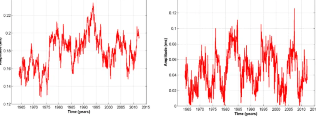
Figure 1. Amplitude of the 0.5-year FFT component of the LOD for different FFT sliding windows (2τ ): 1 year (A), 2 years (B), 4 years (C)

and 8 years (D).

1992; Le Mouël et al., 2010). Original data are taken from the database of the International Earth Rotation and Ref-erence System Service (IERS), of the Earth Rotation Cen-ter at Paris Observatory (http://hpiers.obspm.fr/eoppc/eop/ eopc04/eopc04_IAU2000.62-now). The analysed data set was obtained using calculations described by Le Mouël et al. (2010). After preprocessing, the resulting data set cov-ers the time interval from January 1964 to March 2012. The main goal of preprocessing was to extract from the original data set, containing oscillations at various frequencies, the semi-annual LOD variation. In particular, to eliminate the strong irregular longer-term variation, the further steps were done. Simple linear trend can be removed by simply subtract-ing a least-squared-fit (or first-degree polynomial fit) straight line. However, LOD variation results from geophysical phe-nomena and most geophysical quantities have red spectra, which imply more low-frequency variability than we would find simply in a linear trend. In addition as the linear trend does not fully explain the red spectrum, we may still be con-cerned about edge effects on the spectrum. One way to min-imize the impact of the red spectrum and therefore the edge effect on the FFT is to compute the time derivative of the data. Finally the time derivative has the property of not in-terfering with the time series; that is, we neither assume a particular model for those low frequencies nor apply a par-ticular low-pass filter.

A derivative of the original data set of the daily values of LOD was calculated for each day k. As a result we obtained

the data set lod0(k). Next, for each day k we calculated Fourier coefficients C(k) corresponding to the 0.5-year (T ) spectral line. For this calculation we used a 4-year (2τ ) slid-ing window width which was centred on each day k.

C(k) = A(k) + iB(k)

=1t /(2τ + 1)6_ρ=k−τρ=k+τlod0(k)(cos(ωρ) + i sin(ωρ)),

where ω = 360◦/T (in degrees per day), T = 0.5 year (182.62 days), τ = 2 years (730 days), and 1t = 1 day is the sampling interval.

An amplitude α(k) of the 0.5-year variation of the lod0can be estimated as a module of the FFT amplitude multiplied by the factor of T /2π :

α(k) = (182.62/2π ) · A(k),

where A(k) = (A2(k) + B2(k))1/2.

Two questions can be raised at this point: one technical, the other physical. The first is related to a possible dependence resulting from the choice of the FFT sliding window. Fig-ure 1 presents four curves of 0.5-year LOD oscillation that have been calculated using different FFT sliding windows: 1 year (graph A), 2 years (graph B), 4 years (graph C) and 8 years (graph D). Graph C shows a very clear 11-year vari-ability. Graphs A and B show observable 11-year variability, but visible noise must be filtered out. Graph D also shows 11-year variability, but its relative amplitude is lessened. Hence,

(5)

Figure 2. Oscillations of the LOD data set with different periods: 1 year (A) and 2 years (B). FFT-window width remains unchanged at

4 years.

for our investigation we chose the 4-year FFT sliding win-dow width as optimal (Graph C).

The second question is related to the LOD oscillation that exhibits the 11-year cycle. Figure 1c depicts the 0.5-year oscillation of LOD showing 11-year variability. Figure 2 presents two other LOD oscillations: the first over 1 year (Graph A) and the second over 2 years (Graph B). In both cases we used an FFT sliding window width of 4 years. Even if variations of 1-year LOD oscillation do show some peri-odicity around 11 years, this trend is less clear than that de-scribed above for the 0.5-year oscillation of LOD in Fig. 1c. The graph presented in Fig. 2b demonstrates no clear cyclic-ity around 11 years.

Consequently, for this study we have thus focused on the 0.5-year oscillation of LOD, as presented in Fig. 1c. This data set covers solar cycles 20 to 23. Hereafter, it is referred to simply as LOD. Our study of variations of LOD requires additional data sets of SA and of CRI covering a time interval as long as the LOD data set.

2.2 Solar activity – sunspot number (SSN)

As a simple and robust parameter characterizing SA varia-tions, we used the monthly index of sunspot numbers (SSNs, from the Solar Influence Data Center (SIDC) database). The data set is extensive, starting in 1749 and continuing until the present. This data set may be too rough as a proxy of SA. Another index such as the total solar irradiance (TSI, in W m−2) is certainly preferable, but it covers a shorter time in-terval from 1975 to 2003 (Composite Total Solar Irradiance database 1978–present, compiled by C. Fröhlich and J. Lean; Fröhlich, 2003). The 1978 to 2003 portion of the data set is based on observed data, and the 1975 to 1978 portion is based on modelled data. Both (SSN and TSI) extended data sets can be found in the NGDC-NOAA database (SSN – http://www. ngdc.noaa.gov/stp/solar/ssndata.html, TSI – ftp://ftp.ngdc. noaa.gov/STP/SOLAR_DATA/SOLAR_IRRADIANCE/).

In this study we use the longer SSN index for SA. How-ever, in order to show how the solar activity related to be-haviour of the TSI, we present both data sets in Fig. 3 (top graph) (the original data sets and the smoothed version by ad-jacent averaging with a window of 30 months). It can be seen that both data sets exhibit very similar behaviour over the nearly 11-year period (Schwabe). As expected, the smoothed curves clearly show that Schwabe cycle maxima for the TSI and SSN correspond precisely. Relative amplitudes of the cy-cles can differ: for example, in SSN (smoothed data set) am-plitudes of solar cycles 21 and 22 are higher (about 150) than the one of solar cycle 23 (about 100), but in TSI (smoothed data set) this difference is less (about 1366.3 W m−2for the cycles 21, 22 and about 1366.4 for the cycle 23). Neverthe-less, the dates of extremes (minimal and maximal points) of the solar cycles presented by SSN and TSI are similar.

2.3 Cosmic ray intensity (CRI)

As an indicator of CRI, we use two data sets describing the number of counts recorded by two different neutron mon-itors. The first record, from the CLIMAX neutron moni-tor, spans the interval from January 1951 to October 2006 (http://www.ngdc.noaa.gov/stp/spaceweather.html). The sec-ond, from the McMurdo neutron monitor, spans the inter-val from January 1965 to September 2013 (http://neutronm. bartol.udel.edu/). Using these two data sets we can consider the time interval, which fully or partially covers solar cycles 19 to 23. However, the LOD data only cover solar cycles 20– 23, preventing us from analysing solar cycle 19.

2.4 Preprocessing of original data sets

The data sets analysed for this study were preprocessed as follows. (1) The data sets were smoothed by adjacent aver-aging with a window of 30 months. This window dimension was chosen as being optimal for an approximation of the original data sets. The choice of a smaller window dimen-sion allows the analysis of oscillations of higher frequencies, which can be of interest in the investigation of links between

(6)

Figure 3. Original data and data smoothed by adjacent averaging

(30 months) of SSN, TSI (W m−2), CRIInv(CLIMAX (red lines) and McMurdo (magenta lines)) and LODInv. The curves for the common time interval are presented. Solar cycles (from 20 to 23) are indicated at the bottom of the figure.

different processes. However, for our study focused on 11-year variations, a sliding window size of 30 months gives us a good approximation. Original and smoothed curves are presented in Fig. 3. (2) The resulting curves were then de-trended by correcting for a linear trend. The final time series (Fig. 4) were then obtained by normalization of the smoothed and detrended records.

3 Methodology

One of our objectives is to calculate phase lag values for pairs of different parameters. Since we consider phase lag evolution between 11-year cycles, we should first demon-strate the presence of variations with such a period in each of the analysed data sets. We used wavelet analysis to ob-tain a spectrum in which a time evolution can be seen. This method is very effective not only for the analysis of lin-ear, stable signals but also for the analysis of nonlinlin-ear, un-stable signals. Basic principles, peculiarities and some ex-amples of using the wavelet analysis are presented in Tor-rence and Compo (1998). The mathematical definition of the wavelet transform (W ) of time sequence xn(n =0. . .N ) with step 1t is the following: Wn(s) = P

n0₌_{0:N −1}

xn0ψ ∗[(n0−

n)1t /s], where ψ is a localized wavelet, s is a scale pa-rameter and n is a time index, and asterisk denotes com-plex conjugation. Here we use the Morlet wavelet 9(η) =

π−1/4exp(iω0η)exp(−η2/2), where ω0=6 and η is a

di-mensionless time parameter.

The result can be visualized by a figure presenting wavelet spectrum of the analysed signal. The colourmap used in the figure corresponds to the amplitudes of the wavelet spectrum.

Figure 4. Normalized curves of smoothed (Fig. 3) and linearly

de-trended data of SSN, CRIInv(CLIMAX (red lines) and McMurdo (magenta lines)) and LODInv. The curves for the common time in-terval are presented. Solar cycles (from 20 to 23) are indicated at the bottom of the figure.

Statistical significance is calculated as a 5 % significance level against the red noise background. Statistically signifi-cant zones of the spectrum are contoured by a black line. An influence of boundary effects is taken into account: one has to trust only results inside the so-called “cone of influence”. On the wavelet spectrum the zones outside the cone are shad-owed.

Since we analyse cycles which originated through pro-cesses of different nature and which may have been influ-enced by different factors, it is possible that the length of the cycles may differ. Because of this, any choices made con-cerning the method of phase lag analysis are important. To comply with this we have used different techniques in order to make phase lag calculations as accurate as possible. First, the pair of cycles corresponding to the same solar cycle was chosen; next, the phase lags between the two cycles were cal-culated using

– the difference between dates of maximal amplitudes of

the two cycles

– the phase lag which corresponds to the maximum

cor-relation coefficient between the two cycles

– the phase lag calculated from cross-recurrence plots.

3.1 Brief description of methods used for phase lag analysis

There are different methods that can serve to estimate phase lag between two data sets for each solar cycle. The first

(7)

one consists of methods allowing the discrete calculation of phase lag and is used, for example, to determine phase lag at the dates of maximal amplitudes of the two cycles. A sec-ond technique allows the computation of average phase lag for a chosen time interval (e.g. a particular solar cycle) and can be used, for example, to estimate phase lag correspond-ing to a maximal value of the correlation coefficient. The last method allows estimating phase lag between two analysed data sets for each point (date). Cross-recurrence plot analysis can serve as an example of this method. This last method is very effective in the analysis of data sets between which the coherence is not stable.

The analysis of a recurrence plot of a data set is based on the idea of recurrence as a fundamental property of each dynamical system and on the idea of the possibility to in-vestigate the behaviour of a system based on an understand-ing of its phase-space behaviour in Takens’ theorem (Takens, 1981). Phase-space behaviour of x(t ) can be reconstructed using Xi=(xi, xi+τ, . . ., xi+(m−1)τ), where m is the

embed-ding dimension and τ is the time delay.

Topological structures of the original data set xi are guar-anteed to be saved if m ≥ 2d + 1, where d is a dimension of the attractor (Takens, 1981). A cross-recurrence plot analy-sis is based on the same idea but allows analysing dependen-cies between two data sets. Let us consider two dynamical systems presented by vectors xi and yi in a d-dimensional phase space. The systems are shown by two data sets xi and

yi, where i = {1, . . ., N } and j = {1, . . ., M}. N is a number of states of xi, and M is a number of states of yi. Mathemat-ically, a matrix of cross-recurrence (CRx,y_i,j)of these two data sets can be defined as follows:

CRx,y_i,j (ε) = 2(εi− ||xi−yj||), where i = {1, . . ., N } , j = {1, . . ., M} .

|| · ||is a norm, εi is a threshold distance (a radius of a cho-sen neighbourhood of xi)and 2(·) is the Heaviside func-tion which is equal to 1 or to 0. If vector yj is outside the neighbourhood of vector xiwith a radius of εi, then 2(εi− ||

xi−yj||) is equal to 0. Otherwise, 2(εi− ||xi−yj||) is equal to 1.

The matrix of cross-recurrence can be visualized as a cross-recurrence plot. This is an (i, j ) coordinate system. An “image” consists of black and white points: if 2 for a chosen pair (i, j ) is equal to 1, then a corresponding point is black; if it is equal to 0, then a corresponding point is white. The evo-lution of phase lag can be estimated using line of synchro-nization (LOS). It can be constructed on a cross-recurrence plot from the bottom left corner to the upper right corner (in the direction of an arrow of time) in agreement with the highest density of cross-recurrence points. The choice of parameters used for the construction of a cross-recurrence matrix is important. In this paper we present results ob-tained using the “fixed distance maximal norm” (L∞), em-bedding dimension m = 1, time delay τ = 1 and ε = 0.1σ ,

where σ is the standard deviation. A detailed description of cross-recurrence-plot analysis can be found in Marwan et al. (2007). In this study we used the package for MAT-LAB that can be found at http://www.agnld.uni-potsdam.de/ ~marwan/toolbox/.

3.2 Determination of solar cycle limits

The determination of cycle limits (start and end dates) poses a problem because it can be obtained using different meth-ods. The first method considers a cycle as an interval between the two nearest minima of solar activity. A second possible method is based on the analysis of a trajectory of an investi-gated data set in phase space (2-D diagram method; Usoskin et al., 2001; Takens’ theorem; Takens, 1981). As mentioned above, the starting and ending points of a cycle are deter-mined by the closeness of circles in phase space. Cycle limits obtained in this manner can differ from the limits of cycles found as nearest minima.

In this work we determine the limits of solar cycles as a time interval between two nearest minima of solar activity. We have chosen not to consider the method based on 2-D diagrams because of the difficulties involved in applying this method to the LOD data set discussed above.

4 Results

In this section we present the results of our investigation based on the visual analysis and relationships of curve shapes and on the analysis of phase lags between SSN, CRI (for the CLIMAX and McMurdo neutron monitors) and LOD for so-lar cycles 20–23. We start this section with the list of chosen limits of solar cycles.

4.1 Limits of solar cycles

We use the following periods as solar cycle minima in agree-ment with the determination of a solar cycle as an interval between two closest minima of SA: cycle 20 from 1964 to 1975, cycle 21 from 1975 to 1986, cycle 22 from 1986 to 1996, and cycle 23 from 1996 to 2008.

We have found minima of solar activity for the curves pre-sented in Fig. 4 with a precision of about a month. Although solar cycle 23 is not complete in the LOD data set (Figs. 3 and 4), we analyse it in a similar way, because the use of par-ticular methods (for example comparison of maximal points of cycles) can lead to precise estimations of phase lag, and because the use of other methods (maximal coefficient of cross-correlation and recurrence plot analysis) allows prelim-inary estimations.

4.2 Shape of curves: visual and wavelet analysis

Figure 3 presents monthly variations of SA (SSN and TSI), inverted CRI and inverted LOD. Smoothed curves are

(8)

Figure 5. Wavelet spectra of the data presented in Fig. 3 for the time interval closed to analysed: SSN (A), LOD (B), CRIInv(CLIMAX – C, McMurdo – D). Y axes present periods in years. Wavelet amplitudes are shown by different colours, accordingly to colourmaps.

represented in the same figure with solid lines. The curves presented cover the time interval from 20 to 23 solar cy-cles (fully or partially). Figure 4 illustrates the same data sets as Fig. 3 (except for TSI), but the data sets have been pre-processed as discussed above (Sect. 2): they have been smoothed, detrended and normalized. Here we analyse the smoothed and normalized curves presented in Fig. 4 for so-lar cycles 20 to 23. Further on in this article, we name these data sets “SSN”, “CRI” and “LOD”.

A visual analysis of the curves presented in Fig. 4 shows that all data sets investigated reveal an approximate 11-year variability. To confirm an existence of 11-year variability in all analysed data sets, we applied wavelet analysis to each of the data sets presented in Fig. 4. The corresponding wavelet spectra are presented in Fig. 5. Even if the available time interval is relatively short, one can clearly see statistically significant and stable signals with about 11-year period for all analysed data sets: SSN (A), LOD (B) and CRI (CLIMAX – C, McMurdo – D).

However, as it can be seen from Figs. 3 and 4, each curve demonstrates peculiarities, the comparison of which enables us to propose preliminary suggestions concerning the rela-tionships between the parameters. One such specific inter-val occurs from 1970 to 1980 (Fig. 4). A smooth decrease of SSN can be observed between 1970 and 1975. However, the CRI curve shape for the same time interval demonstrates more complex and irregular behaviour than does the SSN curve. The shape of the LOD curve also shows some com-plexity.

Another peculiarity can be observed between 1985 and 1990. From Fig. 4 it can be seen that, for the LOD data set, the minimum between solar cycles 21 and 22 is higher than its neighbouring minima (between cycles 20 and 21, and be-tween cycles 22 and 23). In the case of SSN, these three minima reach the same level. Both CRI minima between so-lar cycles 21 and 22 exhibit values slightly higher than their neighbouring minima but not as much as in the case of LOD.

4.3 Phase lag analysis: maxima, maximal correlation coefficient, cross-recurrence plots

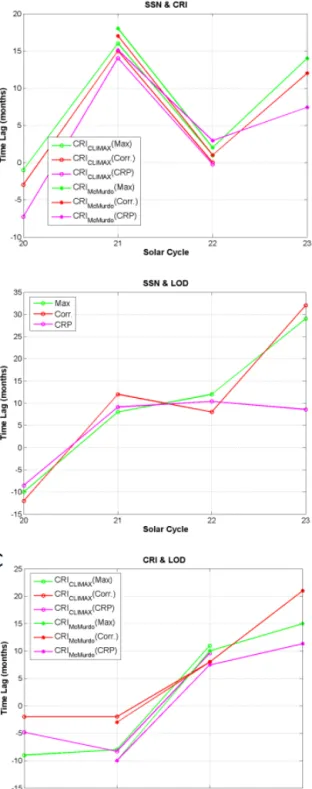
In Fig. 6 we present phase lags calculated for SSN, CRI (CLIMAX and McMurdo neutron monitors) and LOD data sets for solar cycles 20–23. An estimation of phase lag was achieved using three different methods: comparison of max-ima, analysis of maximal correlation coefficient and with the cross-recurrence plot method. Graph A shows phase lag evo-lution between SSN and CRI, Graph B depicts SSN and LOD and Graph C illustrates CRI and LOD.

It should be noted that the results obtained using the three different methods are very similar (Fig. 6), even in the case of solar cycle 23 with its incomplete LOD record. In Fig. 6, the top graph (A) demonstrates very clear differences in phase lags for even and odd solar cycles between SSN and CRI for both neutron monitors. The middle graph (B) and bottom graph (C) show a positive trend in phase lags between SSN and LOD as well as between the CRI of both neutron moni-tors and LOD. It can be seen that the phase lags presented on

(9)

Figure 6. Time lags (in months) between normalized data sets

pre-sented in Fig. 4 calculated using different methods for (A) SSN and CRIInv, (B) SSN and LODInvand (C) CRIInvand LODInv. Solar cycles are from 20 to 23. The limits of the cycles are considered as minima of curves. For each pair, positive lag means that the first parameter is ahead of the second one, and negative is the opposite.

graphs B and C of Fig. 6 demonstrate not only a positive in-crease, but that they also illustrate some additional variations of phase lags for even and odd solar cycles. What is partic-ularly interesting is the observation that, for solar cycle 20, the phase lags between pairs of the investigated parameters (SSN and LOD, CRI and LOD) are negative. The apparent negative phase lags between SA and CRI could be explained if the recovery of CR intensity is faster than a declining rate of SA level (Usoskin et al., 2001). But the origin of the neg-ative phase lag between SSN and LOD, as well as between CRI and LOD, is still a matter of discussion.

5 Discussion

In addition to being of relevance to phase lag evolution be-tween parameters such as SSN, CRI and LOD, the results presented in this paper also provide arguments supporting or refuting proposed mechanisms of the influence of solar activ-ity on the Earth’s rotation. The shape of the curves of SSN, CRI and LOD presented in Fig. 4 as well as the phase lags between these parameters can be discussed in this context.

As shown in Fig. 4 the beginning of cycle 22 in LOD oc-curs earlier than in CRI but a bit later than in SSN. For the few years preceding 1975, both the LOD curve and the CRI curves exhibit complicated shapes. In addition, the beginning of cycle 20 in LOD occurs earlier by about 2–10 months than it does in CRI, but slightly later by about 7–12 months than it does in SSN (as was observed above for the 1985–1990 time interval). Moreover, the shape of the LOD curve around 1977 shows greater similarity to the shape of the SSN curve than to the shape of CRI curves. These differences may not be com-patible with the hypothesis that the Sun influences LOD via the modulation of cosmic rays.

It is also remarkable that the minimum value of the LOD curve is higher around 1987 than it is for the 1977 and 1997 minima. A similar effect (with slightly less difference be-tween the three minima) can be observed for the CRI curves but not for the SSN curve. The respective shapes of the SSN, CRI and LOD curves around and after the 1997 minimum cannot be considered as conclusive facts supporting or refut-ing the hypothesis that SA influences LOD via CRI.

An analysis of phase lags between SSN, CRI and LOD can also be useful to identify or rule out possible mecha-nisms. The results presented in Fig. 6a show that the phase lag between SSN and CRI is large for odd solar cycles and negligible or even negative for even solar cycles. This result confirms results by previous authors (Nymmik and Suslov, 1995; Usoskin et al., 2001; Gupta et al., 2006; Mishra et al., 2006; and Mavromichalaki et al., 2007). Although a negative phase lag for solar cycle 20 (see Fig. 6a) is counter-intuitive, it is nevertheless linked to physics. As discussed by Usoskin et al. (2001), the duration of the recovery phase of CRI mod-ulated by SA in solar cycle 20 was unusual and the phase lag between SSN and CRI is negative for this cycle. It implies

(10)

that the recovery of cosmic ray intensity during cycle 20 was faster than sunspot activity (Usoskin et al., 2001). Accord-ing to these authors, it could have happened because of the unusual reversal of the global solar magnetic field leading to an unusual heliospheric structure. Soon after the maximum of solar cycle 20, the heliosphere became rather quiet. More-over, it was relatively “thin” for energetic particles (above some 13 GeV) but still thick for low-energy cosmic rays. These reasons could lead to a long flat maximum of cosmic ray intensity and to an energy-dependent modulation during solar cycle 20 (see details in Usoskin et al., 2001, and refer-ences therein).

However, the results presented in graphs B and C of Fig. 6 concerning the phase lags between SSN and LOD and be-tween CRI and LOD are less clear and not simple to interpret. It can be said that phase lags demonstrate a positive trend in both cases. Nevertheless, cycle 20 phase lags are significantly negative in both cases.

The arguments based on visual shape analysis allow us to put forward a preliminary suggestion that the behaviour of the LOD curve is more similar to that of the SSN curve than it is to that of CRI curves. This can be considered as an ar-gument in support of the hypothesis that the Earth’s rotation may be influenced by solar activity, but presumably not via the fluctuations of cosmic rays. A goal of this article is to analyse the solar activity as a possible driver of the semi-annual LOD variability. As mentioned in Sect. 2.1 of this paper, the seasonal cycle is one of the largest components of the LOD variability and, within the semi-annual oscilla-tion, presents a prominent decadal modulation (Bourget et al., 1992; Le Mouël et al., 2010). But for the moment its ori-gin, as well as the respective roles of various internal and external causes, remains under discussion.

For example, Abarca del Rio et al. (2003), investigat-ing the lower frequencies in LOD and AAM (i.e. filterinvestigat-ing out seasonal variability, so not discussing the modulation of the seasonal cycle), suggested that AAM variability at the decadal timescales close to the solar cycle can originate from surface processes with the troposphere contribution to the total power being of about 80 %. However, the same au-thors mention that the global AAM data set at this 11-year timescale shows a significant phase lag with solar activity – about 2 months on average – over the last 50 years. Moreover, some studies (see Abarca del Rio et al., 2003, and references therein) show at least a partial agreement between solar activ-ity and independent measurements (sea surface temperature, global temperature (GT), AAM, LOD) over the last 50 years while being out of phase at the beginning of the 20th century. Moreover, multiple signals having distinct origins within the atmosphere with about the same frequency band as the 11-year solar cycle can impact global AAM and interfere with the solar signal (Abarca del Rio et al., 2003), complicating a precise detection of solar forcing.

For this reason, the role of the solar forcing in zonal wind redistribution cannot be ruled out. Its instability may be

related to additional internal or external factors or to the infe-rior quality of the observational data in the past (see Abarca del Rio et al., 2003, and references therein). In addition to the explanation involving zonal wind redistribution, there are other factors, which may lead to changes in Earth angular momentum (inner Earth processes as evidenced recently by Holme and Viron, 2013). But the discussion of these factors is beyond the scope of this article.

6 Conclusions

Using different methods (comparison of maxima of 11-year cycles, analysis of correlation coefficients and cross-recurrence plots) we confirm systematic differences of phase lag values between solar activity (SA) and cosmic ray inten-sity (CRI) for even and odd solar cycles. We also show that phase lags for even solar cycles are small or even negative (from −7 to +3 months), whereas phase lags for odd solar cycles are relatively large (from +6 to +18 months).

We determine that, for solar cycle 20, phase lags between pairs of the investigated parameters (SA and LOD, CRI and LOD) are significantly negative. Using the same methods of analysis, we investigated phase lags between SA and LOD as well as between CRI and LOD for cycles 20 to 23. We found clear positive long-term trends in phase lags. More-over, some additional variations of phase lag values were also observed. The trend shows the instability of the phase rela-tionship, casting doubts on the existence of a simple solar origin of the 11-year cycle in the LOD record.

We interpret the results from the point of view of pos-sible mechanisms governing the influence of solar activity on the Earth’s rotation. The short length of the records does not allow deriving a definitive conclusion about a particular mechanism. However, results are not particularly supportive of an influence of cosmic rays on LOD variations. Indeed, the phase lag observed between SA and LOD does not show any clear difference between odd and even solar cycles as would be predicted if cosmic rays were the main forcing.

Acknowledgements. The authors are grateful to Ilya Usoskin for a fruitful discussion.

Topical Editor E. Roussos thanks two anonymous referees for their help in evaluating this paper.

References

Abarca del Rio, R., Gambis, D., Salstein, D., Nelson, P., and Dai, A.: Solar activity and earth rotation variability, J. Geodyn., 36, 423–443, 2003.

Abarca del Rio, R., Gambis, D., and Salstein, D. A.: Interannual sig-nals in length of day and atmospheric angular momentum, Ann. Geophys., 18, 347–364, doi:10.1007/s00585-000-0347-9, 2000.

(11)

Aoyama, Y. and Naito, I.: Wind contributions to the Earth’s angular momentum budgets in seasonal variation, J. Geophys. Res., 105, 12417–12431, 2000.

Bourget, P., Gambis, D., and Salstein, D.: Possible relationships be-tween Solar activity, atmospheric variations and Earth Rotation, in: Journées 1992 “Systèmes de référence spatio-temporels”, edited by: Capitaine, N., 172–176, 1992.

Challinor, R. A.: Variations in the rate of rotation of the Earth, Sci-ence, 172, 1022–1024, 1971.

Chao, B., Chung, W., Shin, Z., and Hsieh, Y.: Earth’s ro-tation variations: a wavelet analysis, Terra Nova, in press, doi:10.1111/ter.12094, 2014.

Chapanov, Y. and Gambis, D.: Correlation between the solar activity cycles and the Earth rotation, Proc. Journées 2007 “Systèmes de Référence Spatio-Temporels”, edited by: Capitaine, N., Obs. de Paris, 206–207, 2008.

Chapanov, Y. and Gambis, D.: Solar-terrestrial energy transfer dur-ing sunspot cycles and mechanism of Earth rotation excitation, Proceedings of the International Astronomical Union, 264, 119– 121, 2009a.

Chapanov, Y. and Gambis, D.: Changes of the Earth moment of inertia during the observed UT1 response to the 11-year solar variation, Proc. Journées 2008 “Systèmes de Référence Spatio-Temporels”, edited by: Soffel, M. and Capitaine, N., Lohrmann-Observatorium and Obs. de Paris, 131–132, 2009b.

Currie, R. G.: Solar cycle signal in Earth rotation: nonstationary behavior, Science, 211, 386–389, 1981.

Danjon, A.: Sur les variations de la rotation de la Terre et sur une cause possible de la variation aléatoire, C. R. Acad. Sci., 247, 2061–2066, 1958.

Danjon, A.: La rotation de la Terre et le Soleil calme, C. R. Acad. Sci., 254, 3058–3061, 1962.

Eubanks, T. M.: Variations in the orientation of the Earth. In: Con-tributions of Space Geodesy to Geodynamics, Earth Dynamics, edited by: Smith, D. E. and Turcotte, D. L., American Geophys-ical Union Geodynamics Series, 24, Washington, D.C., 1–54, 1993.

Fröhlich, C.: Solar Irradiance Variability, in: Chapter 2 of Geophys-ical Monograph Series, 111, American GeophysGeophys-ical Union (since version 25), 2003.

Gambis, D.: André Danjon, variations de la rotation de la Terre et activité solaire, Proc. Journées Systèmes de Référence Spatio-Temporels, Colloque André Danjon, Obs. Paris, 177–182, 1990. Gray, L. J., Beer, J., Geller, M., Haigh, J. D., Lockwood, M., Matthes, K., Cubasch, U., Fleitmann, D., Harrison, G., Hood, L., Luterbacher, J., Meehl, G. A., Shindell, D., van Geel, B., and White, W.: Solar influences on climate, Rev. Geophys., 48, RG4001, doi:10.1029/2009RG000282, 2010.

Gross, R. S.: Earth Rotation Variations – in Physical Geodesy, edited by: Herring, T. A., Treatise on Geophysics, 11, Elsevier, Amsterdam, 2007.

Gross, R. S., Marcus, S. L., Eubanks, T. M., Dickey, J. O., and Kep-penne, C. L.: Detection of an ENSO signal in seasonal length-of-day variations, Geophys. Res. Lett., 23, 3373–3376, 1996. Gross, R. S., Marcus, S. L., and Dickey, J. O.: Modulation of the

seasonal cycle in length-of-day and atmospheric angular momen-tum, in Proceedings of IAG Symposia, 2001: Vistas for Geodesy in the New Millennium, 125, 457–462, 2002.

Gupta, M., Mishra, V. K., and Mishra, A. P.: Long-term Modulation of Cosmic Ray Intensity in relation to Sunspot Numbers and Tilt Angle, J. Astrophys. Astr., 27, 455–464, 2006.

Hathaway, D. H.: The Solar Cycle, Living Rev. Solar Phys., 7, 1–59, 2010.

Hide, R., and Dickey, J. O.: Earth’s variable rotation, Science, 253, 629–637, 1991.

Holme, R. and de Viron, O.: Characterization and implications of intradecadal variations in length of day, Nature, 499, 202–204, 2013.

Höpfner, J.: Seasonal variations in length of day and atmospheric angular momentum, Geophys. J. Int., 135, 407–437, 1998. Höpfner, J.: Atmospheric, oceanic and hydrological contributions

to seasonal variations in length of day, J. Geodesy, 75, 137–150, 2001.

Jin, S., Zhang, L. J., and Tapley, B. D.: The understanding of length-of-day variations from satellite gravity and laser ranging mea-surements, Geophys. J. Int., 184, 651–660, 2011.

Kudela, K., Mavromichalaki, H., Papaioannou, A., and Gerontidou, M.: On mid-term periodicities in cosmic rays, Solar Phys., 266, 173–180, 2010.

Le Mouël, J.-L., Blanter, E., Schnirman, M., and Courtillot, V.: So-lar forcing of the semi-annual variation of length-of-day, Geo-phys. Res. Lett., 37, L15307, doi:10.1029/2010GL043185, 2010. Li-Hua, M. and Yan-Ben, H.: Atmospheric Excitation of Time Vari-able Length-of-Day on Seasonal Scales, Chinese J. Astron. Astr., 6, 120–124, 2006.

Marwan, N., Carmen Romano, M., Thiel, M., and Kurths, J.: Re-currence Plots for the Analysis of Complex Systems, Phys. Rep., 438, 237–329, 2007.

Mavromichalaki, H., Belehaki, A., Rafios, X., and Tsagouri, I.: Hale-cycle effects in cosmic ray intensity during the last four cycles, Astrophys. Space Sci., 246, 7–14, 1997.

Mavromichalaki, H., Preka-Papadema, P., Petropoulos, B., Tsagouri, I., Georgakopoulos, S., and Polygiannakis, J.: Low-and high-frequency spectral behavior of cosmic-ray intensity for the period 1953–1996, Ann. Geophys., 21, 1681–1689, doi:10.5194/angeo-21-1681-2003, 2003.

Mavromichalaki, H., Paouris, E., and Karalidi, T.: Cosmic-Ray Modulation: An Empirical Relation with Solar and Heliospheric Parameters, Solar Phys., 245, 369–390, 2007.

Mishra, A. P., Meera Gupta, and Mishra, V. K.: Cosmic Ray Inten-sity Variations In Relation With Solar Flare Index And Sunspot Numbers, Solar Phys., 239, 475–491, 2006.

Nymmik, R. A. and Suslov, A. A.: Characteristics of galactic cosmic ray flux lag times in the course of solar modulation, Adv. Space Res., 16, 217–220, 1995.

Paouris, E., Mavromichalaki, H., Belov, A., Guischina, R., and Yanke, V.: Galactic cosmic ray modulation and the last solar min-imum, Solar Phys., doi:10.1007/s11207-012-0051-4, 2012. Rosen, R. D.: The axial momentum balance of Earth and its fluid

envelope, Surv. Geophys., 14, 1–29, 1993.

Rosen, R. D. and Salstein, D. A.: Contribution of stratospheric winds to annual and semi-annual fluctuations in atmospheric an-gular momentum and the length of day, J. Geophys. Res., 90, 8033–8041, 1985.

Starr, V. P.: An essay on the general circulation of the Earth’s atmo-sphere, J. Meteorol., 5, 39–43, 1948.

(12)

Takens, F.: Detecting strange attractors in turbulence, in: Dynami-cal Systems and Turbulence, edited by: Rand, D. and Young, L. S., 366–381, Warwick, 1980, Lecture Notes in Mathematics 898, Springer-Verlag, New York, New York, USA, 1981.

Thomas, S. R., Owens, M. J., and Lockwood, M.: The 22-Year Hale Cycle in cosmic ray flux: evidence for direct heliospheric mod-ulation, Solar Phys., 289, 407–421, doi:10.1007/s11207-013-0341-5, 2013.

Torrence, C. and Compo, G. P.: A practical guide to wavelet analy-sis, B. Am. Meteorol. Soc., 79, 61–78, 1998.

Yan, H., Zhong, M., Zhu, Y., Liu, L., and Cao, X.: Nontidal oceanic contribution to length-of-day changes estimated from two ocean models during 1992–2001, J. Geophys. Res., 111, B02410, doi:10.1029/2004JB003538, 2006.

Usoskin, I. G., Mursula, K., and Kananen, H., and Kovaltsov, G. A.: Dependence of Cosmic Rays on Solar Activity for Odd and Even Solar Cycles, J. Astrophys. Astron., 27, 455–464, 2001.