Detecting mistakes in engineering models: the effects of experimental design

Detecting mistakes in engineering

models: the effects of experimental design

The MIT Faculty has made this article openly available.

Please share

how this access benefits you. Your story matters.

Citation

Savoie, Troy B., and Daniel D. Frey. “Detecting Mistakes in

Engineering Models: The Effects of Experimental Design.” Research

in Engineering Design 23, no. 2 (April 2012): 155–175.

As Published

http://dx.doi.org/10.1007/s00163-011-0120-y

Publisher

Springer-Verlag

Version

Author's final manuscript

Citable link

http://hdl.handle.net/1721.1/87699

Terms of Use

Creative Commons Attribution-Noncommercial-Share Alike

Detecting Mistakes in Engineering Models:

The Effects of Experimental Design

Troy B. Savoie

Massachusetts Institute of Technology

77 Massachusetts Ave.

Cambridge, MA 02139, USA

savoie@alum.mit.edu

Daniel D. Frey

Massachusetts Institute of Technology

77 Massachusetts Ave., room 3-449D

Cambridge, MA 02139, USA

danfrey@mit.edu

Voice: (617) 324-6133

FAX: (617)258-6427

Abstract

This paper presents the results of an experiment with human subjects investigating their ability to discover a mistake in a model used for engineering design. For the purpose of this study, a known mistake was intentionally placed into a model that was to be used by engineers in a design process. The treatment condition was the experimental design that the subjects were asked to use to explore the design alternatives available to them. The engineers in the study were asked to improve the performance of the engineering system and were not informed that there was a mistake intentionally placed in the model. Of the subjects who varied only one factor at a time, fourteen of the twenty seven independently identified the mistake during debriefing after the design process. A much lower fraction, one out of twenty seven engineers, independently identified the mistake during debriefing when they used a factional factorial experimental design. Regression analysis shows that relevant domain knowledge improved the ability of subjects to discover mistakes in models, but experimental design had a larger effect than domain knowledge in this study. Analysis of video tapes provided additional confirmation as the likelihood of subjects to appear surprised by data from a model was significantly different across the treatment conditions. This experiment suggests that the complexity of factor changes during the design process is a major consideration influencing the ability of engineers to critically assess models.

Keywords

1. Overview

1.1. The Uses of Models in Engineering and the Central Hypothesis

The purpose for the experiment described here is to illustrate, by means of experiments with human subjects, a specific phenomenon related to statistical design of experiments. More specifically, the study concerns the influence of experimental designs on the ability of people to detect existing mistakes in formal engineering models.

Engineers frequently construct models as part of the design process. It is common that some models are developed using formal symbolic symbol systems (such as differential equations) and some are less formal graphical representations and physical intuitions described by logic, data, and narrative (Bucciarelli, 2009). As people use multiple models, they seek to ensure a degree of consistency among them. This is complicated by the need for coordination of teams. The knowledge required for design and the understanding of the designed artifact are distributed in the minds of many people. Design is a social process in which different views and interests of the various stakeholders are reconciled (Bucciarelli, 1988). As described by Subrahmanian et al. (1993), informal modeling comprises a process in which teams of designers refine a shared meaning of requirements and potential solutions through negotiations, discussions, clarifications, and evaluations. This creates a challenge when one colleague hands off a formal model for use by another engineer. Part of the social process of design should include communication about ways the formal model‟s behavior relates to other models (both formal and informal).

The formal models used in engineering design are often physical. In the early stages of design, simplified prototypes might be built that only resemble the eventual design in selected ways. As a design becomes more detailed, the match between physical models and reality may become quite close. A scale model of an aircraft might be built that is geometrically nearly identical to the final design and is therefore useful to evaluate aerodynamic performance in a wind tunnel test. As another example, a full scale automobile might be used in a crash test. Such experiments are still models of real world crashes to the extent that the conditions of the crash are simulated or the dummies used within the vehicle differ from human passengers.

Increasingly, engineers rely upon computer simulations of various sorts. Law and Kelton (2000) define “simulation” as a method of using computer software to model the operation and evolution of real world processes, systems, or events. In particular, simulation involves creating a computational representation of the logic and rules that determine how the system changes (e.g. through differential equations). Based on this definition, we can say that the noun “simulation” refers to a specific type of a formal model and the verb “simulation” refers to operation of that model. Simulations can complement, defer the use of, or sometimes replace particular uses of physical models. Solid models in CAD can often answer questions instead of early-stage prototypes. Computational fluid dynamics can be used to replace or defer some wind tunnel experiments. Simulations of crash tests are now capable of providing accurate predictions via integrated computations in several domains such as dynamics and plastic deformation of structures. Computer simulations can offer significant advantages in the cost and in the speed with which they yield predictions, but also need to be carefully managed due to their influence on the social processes of engineering design (Thomke, 1998).

The models used in engineering design are increasing in complexity. In computer modeling, as speed and memory capacity increase, engineers tend to use that capability to incorporate more phenomena in their models, explore more design parameters, and evaluate more responses. In physical modeling, complexity also seems to be rising as enabled by improvements in rapid prototyping and instrumentation for measurement and control. These trends hold the potential to improve the results of engineering designs as the models become more realistic and enable a wider search of the design space. The trends toward complexity also carry along the attendant risk that our models are likely to include mistakes.

We define a mistake in a model as a mismatch between the formal model of the design space and the corresponding physical reality wherein the mismatch is large enough to cause the resulting design to underperform significantly and make the resulting design commercially uncompetitive. When such mistakes enter into models, one hopes that the informal models and related social processes will enable the design team to discover and remove the mistakes from the formal model. The avoidance of such mistakes is among the most critical tasks in engineering (Clausing, 1994).

Formal models, both physical and computational, are used to assess the performance of products and systems that teams are designing. These models guide the design process as alternative configurations are evaluated and parameter values are varied. When the models are implemented in physical hardware, the

exploration of the design space may be guided by Design of Experiments (DOE) and Response Surface Methodology. When the models are implemented on computers, search of the design space may be informed by Design and Analysis of Computer Experiments (DACE) and Multidisciplinary Design Optimization (MDO). The use of these methodologies can significantly improve the efficiency of search through the design space and the quality of the design outcomes. But any particular design tool may have some drawbacks. This paper will explore the potential drawback of complex procedures for design space exploration and exploitation.

We propose the hypothesis that some types of Design of Experiments, when used to exercise formal engineering models, cause mistakes in the models to go unnoticed by individual designers at significantly higher rates than if other procedures are used. The proposed underlying mechanism for this effect is that, in certain DOE plans, more complex factor changes in pairwise comparisons interfere with informal modeling and analysis processes used by individual designers to critically assess results from formal models. As design proceeds, team members access their personal understanding of the physical phenomena and, through mental simulations or similar procedures, form expectations about results. The expectations developed informally are periodically compared with the behaviour of formal models. If the designers can compare pairs of results with simple factor changes, the process works well. If the designers can access only pairs of results with multiple factor changes, the process tends to stop working. This paper will seek evidence to assess this hypothesis though experiments with human subjects.

1.2. The Nature of Mistakes in Engineering and in Engineering Models

“Essentially, all models are wrong, but some are useful” (Box and Draper, 1987). Recognizing this, it is important to consider the various ways models can be wrong and what might prevent a model from being useful. Let us draw a distinction between what we are calling mistakes in models and what is commonly described as

model error.

Model error is a widely studied phenomenon in engineering design. To the extent that simplifying assumptions are made, that space and time are discretized, that model order is reduced, and solutions of systems of equations are approximated, some degree of model error is invariably introduced. Model error can frequently be treated so that bounds can be rigorously formulated or so that model error can be characterized probabilistically. Such errors are not fully known to us during the design process, but we have some realistic hope of characterizing these errors using repeatable, reliable procedures.

By contrast, mistakes in models are much more challenging to characterize. Examples of mistakes in computer models include a wrong subroutine being called within a program, model data being entered with a decimal in the wrong location, or two data elements being swapped into the wrong locations in an array. Mistakes in physical models can be just as common. Mistakes in physical experiments include recording data in the wrong units, installing a sensor in the wrong orientation, or setting the factors incorrectly in one trial or systematically across all trials (by misinterpreting the coding of factor levels). When such a mistake enters a formal model, it is likely to give an answer that is off by an order of magnitude or even wrong in sign (it may indicate the effects of a design change are opposite to the effect that should actually be observed).

It is interesting to consider how frequently there are mistakes in engineering models and how consequential those mistakes might be. Static analyses of software used for simulation of physical phenomena suggest that commercially available codes contain, on average, eight to twelve serious faults per one thousand lines of code (Hatton 1997). Faults in commercial software may cause us to make wrong predictions about phenomena of interest to us. To make matters worse, we may also say it is also a mistake to build a model that omits important phenomena, even those phenomena we never explicitly intended to include. If errors of omission are included as mistakes, then mistakes in formal models must be common and serious, especially in the domains wherein technology is advancing rapidly.

The presence of mistakes in engineering models and the implications for design methodology have been subjects of much research. Error proofing of the design process is one area of development. For example, Chao and Ishii (1997) worked to understand the categories of errors that occur in the design process and studied concepts of Poka-Yoke that emerged from manufacturing and adapted them to the design process. Computer scientists have undertaken significant work on means to avoid bugs or to detect them early. For example, there is quite consistent evidence across empirical studies showing that pair programming positively affects the quality of code (e.g., by reducing frequency of mistakes) (Dyba, et al. 2007) and that the benefits of pair programming are greatest on complex tasks (Arisholm, et al. 2007). Among the most exciting developments in the last few years, is an approach drawing on experience in the field of system safety. As Jackson and Kang (2010) explain “instead of relying on indirect evidence of software dependability from process or testing, the

developer provides direct evidence, by presenting an argument that connects the software to the dependability claim.” Thus there is hope for the development of an empirical basis for mistake avoidance in computer programming, but there are major challenges in successful implementation. Software designers must ensure adequate separation of concerns so that the empirical data from an existing program remain relevant to a new function they are creating.

The structure of the rest of the paper is as follows. Section 2 provides some background to the investigation. This includes some discussion of relevant cognitive phenomena, and descriptions of one-at-a-time experiments and orthogonal arrays. Section 3 describes the experimental protocol. Sections 4 and 5 present and discuss the results of the investigation. Sections 6 and 7 make some recommendations for engineering practice and suggest some ideas for further research.

2. Background

2.1. Frameworks for Model Validation

The detection of mistakes in engineering models is closely related to the topic of model validation. Formal engineering models bear some important similarities with the designs that they represent, but they also differ in important ways. The extent of the differences should be attended to in engineering design – both by characterizing and limiting the differences to the extent possible within schedule and cost constraints.

The American Institute of Aeronautics and Astronautics (AIAA, 1998) defines model validation as “the process of determining the degree to which a model is an accurate representation of the real world from the perspective of the intended uses of the model.” Much work has been done to practically implement a system of model validation consistent with the AIAA definition. For example, Hasselman (2001) has proposed a technique for evaluating models based on bodies of empirical data. Statistical and probabilistic frameworks have been proposed to assess confidence bounds on model results and to limit the degree of bias (Bayarri, et al., 2007, Wang, et al., 2009). Other scientists and philosophers have argued that computational models can never be validated and that claims of validation are a form of the logical fallacy of affirming the consequent (Oreskes, et al., 1994).

Validation of formal engineering models takes on a new flavor when viewed as part of the interplay with informal models that is embedded within a design process. One may seek a criterion of sufficiency – a model may be considered good enough to enable a team to move forward in the social process of design. This sufficiency criterion was proposed as an informal concept by Subrahmanian et al. (1993). A similar, but more formal, conception was proposed based on decision theory so that a model may be considered valid to the extent that it supports a conclusion regarding preference between two design alternatives (Hazelrigg, 1999). In either of the preceding definitions, if a formal model contains a mistake as defined in section 1.1, the model should not continue to be used for design due to its insufficiency, invalidity, or both.

2.2. Cognitive Considerations

The process by which an engineer might detect a modeling mistake can be described in an abstract sense as follows. The engineer presumably has subject-matter expertise regarding behavior of the components of a device under design consideration. Based on this subject matter knowledge, the engineer may be capable of forming a mental model of probable behavior of the device under different, not yet realized conditions. Bucciarelli (2002) refers to this as the “counterfactual nature of designing” and describes an engineer making conjectures such as „if we alter the airfoil shape in this manner, then the drag will be reduced by this percentage‟. When observing a predicted behavior of the device based on a formal model, whether via a physical prototype or a computer simulation, the engineer may become aware of a conflict between results of two models (e.g. the formal mathematical model might indicate the drag rises rather than drops as expected based on a less formal mental model). The process of integrating observed simulation results into a framework of existing mental models may be considered a continuous internal process of hypothesis generation and testing (Klahr and Dunbar 1988). When observed results are in opposition to the mental model, the attentive engineer experiences an expectation violation (which may reveal itself in a facial expression of surprise) and the engineer must resolve the discrepancy before trust in the mental model is restored and work can continue. The

dissonance between formal and informal models can be resolved by changing the mental model (e.g., learning some new physical insights from a simulation). Alternately, the formal mathematical model may need to change; For example, the engineer may need to find and fix a mistake embedded in the formal model.

It is interesting in this context to consider the strategies used by engineers to assess formal models via numerical predictions from an informal model. Kahneman and Tversky (1973) observed that people tend to make numerical predictions using an anchor-and-adjust strategy, where the anchor is a known value and the estimate is generated by adjusting from this starting point. One reason given for this preference is that people are better at thinking in relative terms than in absolute terms. In the case of informal engineering models, the anchor could be any previous observation that can be accessed from memory or from external aids.

The assessment of new data is more complex when the subject is considering multiple models or else holds several hypotheses to be plausible. Gettys and Fisher (1979) proposed a model in which extant hypotheses are first accessed by a process of directed recursive search of long-term memory. Each hypothesis is updated with data using Bayes‟ theorem. Gettys and Fisher proposed that if the existing hypothesis set is low in plausibility, exceeding some threshold, then additional hypotheses are generated. Experiments with male University students supported the model. These results could apply to designers using a formal model while entertaining multiple candidate informal models. When data from the formal model renders the set of informal models implausible, a hypothesis might be developed that a mistake exists in the formal model. This process may be initiated when an emotional response related to expectation violation triggers an attributional search (Stiensmeier-Pelster et al. 1995; Meyer et al. 1997). The key connection to this paper is the complexity of the mental process of updating a hypothesis given new data. If the update is made using an anchor-and-adjust strategy, the update is simple if only one factor has changed between the anchor and the new datum. The subject needs only to form a probability density function for the conditional effect of one factor and use it to assess the observed difference. If multiple factors have changed, the use of Bayes‟ law involves development of multiple probability density functions for each factor, the subject must keep track of the relative sizes and directions of all the factor effects, and the computation of posterior probabilities involves multiply nested integrals or summations. For these reasons, the mechanism for hypothesis plausibility assessment proposed by Gettys and Fisher seems overly demanding in the case of multiple factor changes assuming the calculations are performed without recourse to external aids. Since the amount of mental calculation seems excessive, it seems reasonable to expect that the hypotheses are not assessed accurately (or not assessed at all) and therefore that a modeling mistake is less likely to be found when there are too many factors changed between the anchor and the new datum.

2.3. Experimental Design: Theoretical and Practical Considerations

Engineering models are frequently used in a process of experimentation. If the model is a physical apparatus, then experimental error will be a concern and statistical Design of Experiments (DOE) may be used to structure the uses of the model. If the model is a computer simulation, then specialized techniques for design of computer experiments may be used. In either case, the complexity of factor changes between the experiments will tend to be high. This section reviews one type of statistical design of experiments. As a comparator, we describe One Factor at a Time (OFAT) experiments, which feature very simple changes between experiments.

2.3.1. Fractional Factorial Design and Complexity of Factor Changes

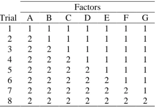
Fractional factorial designs are arrangements of experiments intended to promote efficient exploration and estimation of the effects of multiple factors. An example is the 27-4 design depicted in Table 1, also known as an orthogonal array (Plackett, and Burman, 1946). The labels in the column headings (A through G) represent seven factors in an experiment. The rows represent the settings of the factors for each of eight experimental trials. The entries in each cell indicate the level of the factor, with the labels “1” and “2” indicating two different settings for each factor.

Table 1. A Fractional Factorial Design 27-4.

Factors

Trial A B C D E F G

1

1 1 1 1 1 1 1

2 1 1 1 2 2 2 2

3 1 2 2 1 1 2 2

4 1 2 2 2 2 1 1

5 2 1 2 1 2 1 2

6 2 1 2 2 1 2 1

7 2 2 1 1 2 2 1

8 2 2 1 2 1 1 2

The 27-4 design enables the investigator to estimate the main effects of all seven factors. The design does not enable estimation of interactions among the factors, but two-factor interactions will not adversely affect the estimates using the 27-4 design. Thus, the design is said to have resolution III. It can be proven that using a 27-4 design provides the smallest possible error variance in the effect estimates given eight experiments and seven factors. For many other experimental scenarios (numbers of factors and levels), experimental designs exist with similar resolution and optimality properties.

Note that in comparing any two experiments in the 27-4 design, the factor settings differ for four out of seven of the factors. Relevant to the issue of mistake detection, if a subject employed an anchor-and-adjust strategy for making a numerical prediction, no matter which anchor is chosen, the effects of four different factors will have to be estimated and summed. The complexity of factor changes in the 27-4 design is a consequence of its orthogonality, which is closely related to its precision in effect estimation. This essential connection between the benefits of the design and the attendant difficulties it poses to humans unaided by external aids may be the reason that Fisher (1926) referred to these as “complex experiments.”

Low resolution fractional factorial designs, like the one depicted in Table 1, are recommended within the statistics and design methodology literature for several uses. They are frequently used in screening experiments to reduce a set of variables to relatively few so that subsequent experiments can be more efficient (Meyers and Montgomery 1995). They are sometimes used for analyzing systems in which effects are likely to be separable (Box et al. 1978). Such arrangements are frequently used in robustness optimization via “crossed” arrangements (Taguchi 1987, Phadke 1989). This last use of the orthogonal array was the initial motivation for the authors‟ initial interest in the 27-4 design as one of the two comparators in the experiment described here.

2.3.2. One-at-a-Time Experiments and Simple Paired Comparisons

The one-at-a-time method of experimentation is a simple procedure in which the experimenter varies one factor while keeping all other factors fixed at a specific set of conditions. This procedure is repeated in turn for all factors to be studied. An example of a “one-at-a-time” design with seven different factors (A-G) is given in Table 2. The experiment begins with all the factors set at a baseline setting denoted as “1”. In this particular example, each parameter is changed in turn to another setting denoted “2”. This design is sometimes called a “strict” one-at-a-time plan because exactly one factor is changed from one experiment to the next.

Table 2. A simple version of the “one-factor-at-a-time” method. Factors Trial A B C D E F G 1 1 1 1 1 1 1 1 2 2 1 1 1 1 1 1 3 2 2 1 1 1 1 1 4 2 2 2 1 1 1 1 5 2 2 2 2 1 1 1 6 2 2 2 2 2 1 1 7 2 2 2 2 2 2 1 8 2 2 2 2 2 2 2

This paper will focus not on the simple one-at-a-time plan of Table 2, but on an adaptive one-at-a-time plan of Table 3. This process is more consistent with the engineering process of both seeking knowledge of a design space and simultaneously seeking improvements in the design. The adaptation strategy considered in this paper is described by the rules below:

 Begin with a baseline set of factor levels and measure the response

 For each experimental factor in turn

o Change the factor to each of its levels that have not yet been tested while keeping all other experimental factors constant

o Retain the factor level that provided the best response so far

Table 3 presents an example of this adaptive one-at-a-time method in which the goal is to improve the response displayed in the rightmost column assuming that larger is better.1 Trial #2 resulted in a rise in the response compared to trial #1. Based on this result, the best level of factor A is most likely “2” therefore the factor A will be held at level 2 throughout the rest of the experiment. In trial #3, only factor B is changed and this results in a drop in the response. The adaptive one-at-a-time method requires returning factor B to level “1” before continuing to modify factor C. In trial #4, factor C is changed to level 2. It is important to note that although the response rises from trial #3 to trial #4, the conditional main effect of factor C is negative because it is based on comparison with trial #2 (the best response so far). Therefore factor C must be reset to level 1 before proceeding to toggle factor D in trial #5. The procedure continues until every factor has been varied. In this example, the preferred set of factor levels is A=2, B=1, C=1, D=2, E=1, F=1, G=1 which is the treatment combination in trial #5.

Table 3. An adaptive variant of the one-at-a-time method.

Factors Trial A B C D E F G Response 1 1 1 1 1 1 1 1 6.5 2 2 1 1 1 1 1 1 7.5 3 2 2 1 1 1 1 1 6.7 4 2 1 2 1 1 1 1 6.9 5 2 1 1 2 1 1 1 10.1 6 2 1 1 2 2 1 1 9.8 7 2 1 1 2 1 2 1 10.0 8 2 1 1 2 1 1 2 9.9

The adaptive one-factor-at-a-time method requires n+1 experimental trials given n factors each having two levels. The method provides estimates of the conditional effects of each experimental factor but cannot resolve

1_{Please note that this response in Table 3 is purely notional and designed to provide an instructive example of}

interactions among experimental factors. The adaptive one-factor-at-a-time approach provides no guarantee of identifying the optimal control factor settings. Both random experimental error and interactions among factors may lead to a sub-optimal choice of factor settings. However, the authors‟ research has demonstrated advantages of the aOFAT process over fractional factorial plans when applied to robust design (Frey and Sudarsanam, 2007). In this application therefore, the head-to-head comparison of aOFAT and the 27-4 design is directly relevant in at least one practically important domain. In addition, both the simple and the adaptive one factor at a time experiments allow the experimenter to make a comparison with a previous result so that the settings from any new trial differ by only one factor from at least one previous trial. Therefore, the aOFAT design could plausibly have some advantages in mistake detection as well as in response improvement.

3. Experimental Protocol

In this experiment, we worked with human subjects who were all experienced engineers. The subjects worked on an engineering task under controlled conditions and under supervision of an investigator. The engineers were asked to perform a parameter design on a mechanical device using a computer simulation of the device to evaluate the response for the configurations prescribed by the design algorithms. The subjects were assigned to one of two treatment conditions, viz which experimental design procedure they used, a fractional factorial design or adaptive one-factor-at-a-time procedures. The investigators intentionally placed a mistake in the computer simulation. The participants were not told that there is a mistake in the simulation, but they were told to treat the simulation “as if they received it from a colleague and this is the first time they are using it.” The primary purpose of this investigation was to evaluate whether the subjects become aware of the mistake in the simulation and whether the subjects‟ ability to recognize the mistake is a function of the assigned treatment condition (the experimental procedure they were asked to use).

In distinguishing between confirmatory and exploratory analyses, the nomenclature used in this protocol is consistent with the multiple objectives of this experiment. The primary objective is to test the hypothesis that increased complexity of factor changes leads to decreased ability to detect a mistake in the experimental data. The secondary objective is to look for clues that may lead to a greater understanding of the phenomenon if it exists. Any analysis that tests a hypothesis is called a confirmatory analysis and an experiment in which only this type of analysis is performed is called a hypothesis-testing experiment. Analyses that do not test a hypothesis are called exploratory analyses and an experiment in which only this type of analysis is performed is called a hypothesis-generating experiment. This experiment turns out to be both a hypothesis-testing experiment (for one of the responses) and a hypothesis-generating experiment (for another response we chose to evaluate after the experiment was complete).

The remainder of this section provides additional details on the experimental design. The full details of the protocol and results are reported by Savoie (2010) using the American Psychological Association Journal Article Reporting Standards. The exposition here is abbreviated.

3.1. Design Task

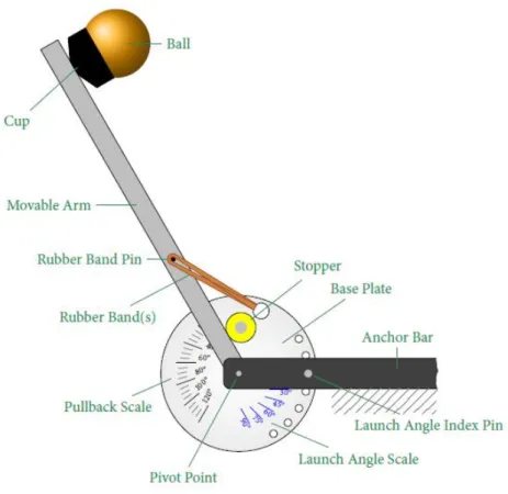
The physical device in the design task is the Xpult catapult (Peloton Systems 2010) shown with component nomenclature in Figure 1. Normal operation of the Xpult catapult is as follows: (1) One or more rubber bands are threaded into the hole in the base plate and wrapped around the rubber band pin, (2) the launch angle is set to one of the values indexed every 15 degrees between 0 and 90, (3) a ball is selected and placed in the cup, (4) the movable arm is rotated to a chosen initial pullback, (5) the arm is released and sends the ball into a ballistic trajectory, and (6) the landing position of the ball is measured. The goal of this parameter design is to find the configuration that results in the ball landing nearest the target distance of 2.44m from the catapult pivot.

Figure 1. A schematic of the X-pult catapult device used in the experiment.

The number of control factors (seven) and levels (two per factor) for the representative design task were chosen so that the resource demands for the two design approaches (the fraction factorial and One Factor at a Time procedures) are similar. In addition to four control factors the Xpult was designed to accommodate (number of bands, initial pull-back angle, launch angle, and ball type), we added three more factors (catapult arm material, the relative humidity, and the ambient temperature of the operating environment). The factors and levels for the resulting system are given in Table 4. The mathematical model given in Appendix A was used to compute data for a 27 full-factorial experiment. The main effects and interactions were calculated. There were 34 effects found to be “active” using the Lenth method with the simultaneous margin of error criterion (Lenth, 1989) and the 20 largest of these are listed in Table 5.

The simulation model used by participants in this study is identical to the one presented in Appendix A, except that a mistake was intentionally introduced through the mass property of the catapult arm. The simulation result for the catapult with the aluminum arm was calculated using the mass of the magnesium arm and vice versa. This corresponds to a mistake being made in a physical experiment by consistently mis-interpreting the coded levels of the factors or mis-labeling the catapult arms. Alternatively, this corresponds to a mistake being made in a computer experiment by modeling the dynamics of the catapult arm incorrectly or by input of density data in the wrong locations in an array.

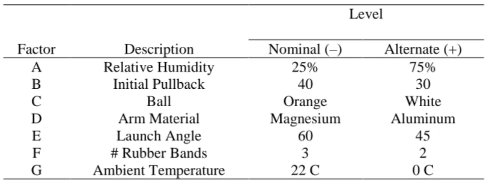
Table 4. The factors and levels in the catapult experiment.

Level

Factor Description Nominal (–) Alternate (+) A Relative Humidity 25% 75% B Initial Pullback 40 30 C Ball Orange White D Arm Material Magnesium Aluminum E Launch Angle 60 45 F # Rubber Bands 3 2 G Ambient Temperature 22 C 0 C

Table 5. The 20 largest effects on landing distance in the catapult experiment.

Term Coefficient F -0.392 B -0.314 D -0.254 E 0.171 C 0.082 B×F 0.034 C×F -0.031 E×F -0.029 G -0.028 B×C -0.025 B×E -0.024 D×F 0.022 B×D 0.022 D×E -0.019 C×D -0.019 F×G 0.009 B×G 0.007 B×C×F 0.007 B×E×F 0.006

3.2. Participant Characteristics

We wanted the experimental subjects to be representative of the actual group to which the results might be applied – practicing engineers of considerable experience. We partnered with Draper Laboratory, a nonprofit, engineering design and development company that operates in a broad range of industries, especially in space and defense. We wanted to ensure the subjects had domain-specific knowledge of simple mechanical dynamics and aerodynamics sufficient to enable them to recognize anomalous behavior when considering the simulation results during the design task. The needed material is typically taught during freshman physics for science and engineering undergraduates, so the minimum eligibility criterion for participating in this study was successful completion of a college-level course in physics including mechanics.

To recruit for this procedure, a person other than the authors contacted approximately 750 potential study participants by email, describing the experiment and inviting those interested to contact the first author directly. All of those contacted were technical staff members of Draper Laboratory with the requisite educational background. Out of the approximately 750 people contacted, 56 of them (about 7.5%) agreed to participate in the study. One of these 56 elected to drop out early in the experiment. Another could not be included in the study because the video tape equipment failed during the experiment. This left 54 subjects in the final group, 27

in each treatment group.

A statistical power analysis determined that a sample size of 25 per each of the two treatment groups would be required to resolve a 3-in-5 chance of becoming aware of a problem versus a 1-in-5 chance. The error rates in this analysis were set at 5% for Type I error (α=0.05) and 10% for Type II error (β=0.10). Thus, the experiment is powered at 90% to resolve the stated effect size. Another consideration is the minimum event count for a good logistic regression fit, and this was assumed to be 10 per covariate in the analysis (Perduzzi et al. 1996).

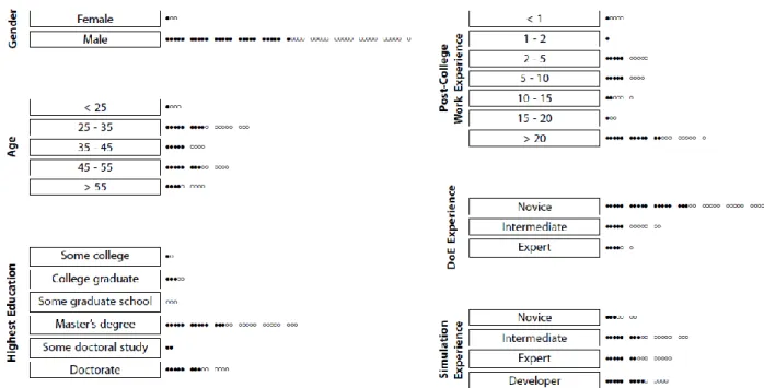
Figure 2. A description of the demographics of the human subjects in the experiment. The filled circles represent subjects in the aOFAT treatment condition and the empty circles represent subjects in the

fractional factorial treatment condition.

The demographics of the participant group are summarized in Figure 2. The engineering qualifications and experience level of this group of subjects was very high. The majority of participants held graduate degrees in engineering or science. The median level of work experience was 12 years. The low number of female participants was not intentional, but instead typical for technical work in defense-related applications. A dozen of the subjects reported having knowledge and experience of Design of Experiments they described as “intermediate” and several more described themselves as “experts”. The vast majority had significant experience using engineering simulations. The assignment of the subjects to the two treatment conditions was random and the various characteristics of the subjects do not appear to be significantly imbalanced between the two groups.

The experiments were conducted during normal business hours in a small conference room in the main building of the company where the participants are employed. Only the participant and test administrator (the first author) were in the room during the experiment. This study was conducted on non-consecutive dates starting on April 21, 2009, and ending on June 9, 2009. Participants in the study were offered an internal account number to cover their time; most subjects accepted but a few declined.

3.3. Measures and Covariates

In this protocol, sixteen measures were taken for each participant: the explanatory variable domain

knowledge score (XDKS), seven instances of the explanatory variable comparison elicits anomaly (XCEA), seven

instances of the exploratory response variable surprise rating (YS), and the confirmatory response variable

debriefing result (YDR).

The explanatory variable XDKS is a measure of the participant‟s level of understanding of the physics of the

change in response when the factor was changed from its nominal to its alternate setting with all other factors held at the nominal setting. The composite score XDKS is the number of predictions in the correct direction. This

explanatory variable was interesting to us as a means of assigning some practical meaning the size of the observed effects. Most of engineering education is related to improving measures similar to the domain knowledge score. This measure would be assumed by most educators and practicing engineers to have an important impact on ability to find and fix mistakes in engineering models. If the choice of experimental design technique has an impact on ability to find mistakes, its relative size compared to domain knowledge score will be of practical interest.

For the second through the eighth trials in the design algorithm, the participant was asked to predict the simulation outcome before being told the result. In each case, the participant was asked which (if any) of the previous results were used in making the prediction. The explanatory variable XCEA is a dichotomous variable

indicating whether the participant based the prediction on one or more trials with the anomalous control factor at the same level (XCEA=0) or at a different level (XCEA=1) than in the configuration being predicted.

The reason for asking participants to make predictions after each trial was to reduce the effects similar to those reported as “automation bias” in the human factors literature (Parasuraman et al. 1993). In developing studies with human experiments such as the ones in this paper, one frequently prescribes an algorithm for each participant to follow. In doing this, errors in judgment may arise. Complacency-induced errors may manifest as inattention of the human participant while carrying out a rigid procedure. One strategy for countering this is to require participants to explicitly predict the response prior to each trial (Schunn and O‟Malley 2000).

The exploratory variable YS is a measure of display of the emotion surprise. Each participant‟s reaction to

being told the simulation result in trials two through eight was videotaped and later judged by two independent analysts on a five-point Likert scale. The analysts were asked to watch the video response, then indicate their level of agreement with the following statement: the subject seems surprised by the result given. Possible answers were Strongly Agree, Agree, Neutral, Disagree and Strongly Disagree. The analysts‟ ratings were subsequently resolved according to the following rules:

 If the raters each selected Strongly Agree or Agree, then the raters were deemed to agree that the subject appears surprised (YS=1).

 If the raters each selected Neutral, Disagree or Strongly Disagree, then the raters were deemed to have agreed that the subject does not appear surprised (YS=0).

 Any other combination of ratings was taken to imply that the raters did not agree, and the data point was not incorporated in the exploratory analysis.

According to Ekman et al. (1987), observing facial expressions alone results in highly accurate judgments of emotion by human raters. However, Russell (1994) points out several serious methodological issues in emotion-recognition studies. We therefore felt it would be prudent to use self-reporting by participants in addition to judgement by independent raters. The confirmatory variable YDR is the response to debriefing at the conclusion

of the experiment. Each participant was asked a series of questions: 1. Did you think the simulation results were reasonable?

2. Those who expressed doubt were asked to pinpoint the area of concern: “Which of the control factors do you think the problem is tied to?”

3. To those who did not express doubt, the administrator then said, “There is a problem in the simulation. Knowing this now, which of the control factors do you think the problem is tied to?”

If the participant‟s answer to the second question is arm material, catapult arm, bar, magnesium versus aluminum, etc. – any wording that unambiguously means the control factor for choice of arm material in the catapult – then the participant was categorized as being aware of the issue (YDR=1); otherwise, the participant

3.4. Experimental Procedure

A flowchart showing the sequence of events during the experiment for each participant is given in Figure 3. This flowchart also shows all explanatory and response variables and the point in the experiment when each is measured or specified.

Fig. 3. Flowchart of experimental method

The experimental process described in Figure 3 was supervised by a test administrator (the first author) who ensured consistent application of the protocol that had been authorized by the Institutional Review Board. All of the subjects were required to undergo what we are calling “device training” in Figure 3. All participants were trained on the operation of the physical device under consideration by listening to a description of the device including the name of each component of the device, the intended operation of the device, and the factors that may be changed in the design task. The “device training” procedure generally required 5 minutes. The graphical aids used by each participant in this study were provided in the form of a sheet of paper and included:

1. On one side, the catapult diagram with components labeled according to nomenclature used in the experiment (which are shown in Figure 2).

2. On the reverse side, the consolidated model reference sheet (which is shown in Appendix B). It should be noted that “device training” was not intended to qualify the person to operate the physical device. It was intended to ensure the subjects understood the nature of the device and the definitions of its operating parameters. We chose not to have people work directly hands-on with the device before working with the simulation of the device. The purpose of the experiment was to assess some challenges related to use of computer simulations in engineering design. In most cases, engineers would not be able to interact with the

exact same physical device before using a simulation to optimize its parameters.

After this “device training”, each participant was instructed to provide, for each of the seven control factors, a prediction of what would happen to the response of the device if the factor were changed from the nominal to the alternate setting, the rationale supporting this prediction, and a level of confidence in the prediction on a scale of 1 to 5 in order of increasing confidence. The accuracy of the predictions and the methodology used by the subjects were assessed and used to develop a domain knowledge score XDKS.

Each participant was told that a computer simulation was to be used in the design task. Each subject was given the exact same description of how it was to be treated. The experiment administrator told each subject to “treat the simulation as if they had received it from a colleague and were running it for the first time.”

Assignments of the participants to control (XDM=0) or treatment (XDM=1) groups were made at random.

Masking was not possible since the treatment variable determined which training was administered. Based on the assignment to a treatment group, training was provided on the design method to be employed.

Participants assigned to the control group used the adaptive one-factor-at-a-time (aOFAT) method. They were instructed to:

1. Evaluate the system response at the nominal configuration. 2. For each control factor in the system

(a) Select a new configuration by using the previously evaluated configuration with the best performance, changing only this factor‟s setting to its alternate value.

(b) Evaluate the system response at the new configuration.

(c) If the performance improves at the new setting of this factor, keep it at this setting for the remainder of the experiment; otherwise, keep it at the original value for the remainder of the experiment.

3. The configuration obtained after stepping through each control factor exactly once is the optimized result for this design approach.

Participants assigned to the treatment group used the fractional factorial design and were instructed to:

1. Evaluate the system response at each of the eight configurations prescribed by the fractional factorial design matrix.

2. Calculate the coefficients in the linear model used to approximate the relationship between the control factors and system response.

3. Using the linear model, find the configuration that results in the best system response. 4. Optionally, check the system response for this configuration using the simulation results. The administrator of the experiment supervised the subjects during the sessions and enforced adherence to these procedures. As an aid in understanding and implementing the design, each participant was also provided with a reference sheet with a summary of the design algorithm and the design table to be used as a worksheet while stepping through the algorithm. In either case, evaluating the system response meant getting the computer simulation result from a lookup table of all possible results. For the fractional factorial design, the estimated responses for the resulting linear model were also provided in tabular form. This approach was taken to reduce the complexity of this experiment and the time required of each participant.

4. Results

4.1. Impact of Mistake Identification during Verbal Debrief

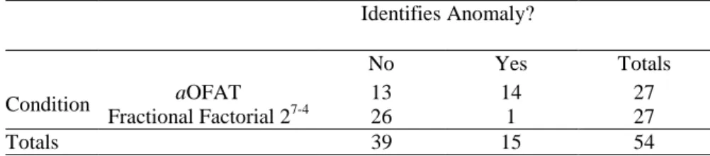
In our experiment, 14 of 27 participants assigned to the control group (i.e., the aOFAT condition) successfully identified the mistake in the simulation without being told of its existence, while only 1 of 27 participants assigned to the treatment group (i.e., the fractional factorial condition) did so. These results are presented in Table 6 in the form of a 2×2 contingency table. We regard these data as the outcome of our confirmatory experiment with the response variable “debriefing result.”

There was a large effect of the treatment condition on the subject‟s likelihood of identifying the mistake in the model. The proportion of people recognizing the mistake changed from more than 50% to less than 4%, apparently due to the treatment. The effect is statistically significant by any reasonable standard. Fisher‟s exact test for proportions applied to this contingency table yields a p-value of 6.3 ×10-5. Forming a two tailed test using Fisher‟s exact test yields a p-value of 1.3 ×10-4

. To summarize, the proportion of people that can recognize the mistake in the sampled population was 15 out of 54. Under the null hypothesis of zero treatment effect, the frequency with which those sampled would be assigned to these two categories at random in such extreme proportions as were actually observed is about 1/100 of a percent.

Table 6. Contingency Table for Debriefing Results Identifies Anomaly? No Yes Totals Condition aOFAT 13 14 27 Fractional Factorial 27-4 26 1 27 Totals 39 15 54

4.2. The Registering of Surprise during Parameter Design

One measure of participant behavior in reaction to the computer simulation result is whether the participant expresses surprise, a well-known manifestation of expectation violation (Stienmeier-Pelster et al. 1995). As this is a subjective measure, it was obtained through ratings by independent judges. Two analysts, with certification in human subjects experimentation and prior experience in a similar study, were hired for this task. The analysts worked alone, viewing the video recordings on a notebook computer using a custom graphical user interface that randomized the order in which responses were shown, enforced viewing the entire response before entering a rating, and collected each rating on a five-point Likert scale.

Applying the decision rule for resolving disagreements between raters as described in section 3.5 resulted in 319 of 385 agreed-upon surprise ratings. In addition to this simple 83% agreement, the margin-corrected value of Cohen‟s kappa (Cohen 1960) was calculated to be 0.708. According to Lombard et al. (2002), these values of simple percent agreement and Cohen‟s kappa are acceptable levels of inter-judge agreement for an exploratory analysis.

These surprise ratings may be used to study the difference in performance between the two treatment groups, by revealing whether the subjects were surprised when they should have been or whether they were surprised when they should not have been. The subjects should presumably be surprised, assuming that prediction ability is sound, when the anomaly is elicited. We define here the anomaly to have been “elicited” when the new result influenced the performance of the device relative to the baseline the subject seemed to be using for comparison. In most cases in this experiment, when a subject made a prediction it was based on an anchor-and-adjust strategy (Tverksy and Kahnemann 1974), where a previously revealed result was used as the anchor. In this particular experiment, the anomaly in the simulation was tied to one factor. Therefore the “anomaly was elicited” when the subject based a prediction on a prior result, and then the parameter was changed so that the anomaly affected the relative performance. In 319 cases, raters agreed on the surprise ratings. In 14 of these 319 cases, it could not be determined unambiguously whether the anomaly had been elicited. All 14 of the ambiguous data points were for the fractional factorial condition and the ambiguity arose when the subject gave more than one anchor and the multiple anchor cases did not have the same value for the factor “arm material”. This left 305 data elements to include in a 2×2×2 contingency table shown in Table 7.

Inspection of the data in Table 7 suggests that those subjects using the aOFAT approach were consistently surprised (22 out of 26 opportunities or 85%) when the anomalous behavior of the model was present in the results they were observing and appeared surprised slightly less than half of the opportunities otherwise. By contrast, subjects using the fractional factorial approach were surprised about half the time whether or not the anomalous behaviour was present.

Table 7. Contingency Table for Surprise Rating Results

Anomaly Surprised?

Elicited? No Yes Totals

Condition aOFAT No 79 52 131 Yes 4 22 26 Fractional Factorial 27-4 No 59 43 102 Yes 24 22 46 Totals 166 139 305

The contingency data are further analyzed by computing the risk ratio or relative risk according to the equations given by Morris and Gardner (1988). Relative risk is used frequently in the statistical analysis of binary outcomes. In particular, it is helpful in determining the difference in the propensity of binary outcomes under different conditions. Focussing on only the subset of the contingency table for the aOFAT test condition, the risk ratio is 3.9 indicating that a human subject is almost four times as likely to express surprise when anomalous data are presented as compared to when correct data are presented to them. The 95% confidence intervals on the risk ratio is wide, 1.6 to 9.6. This wide confidence interval is due to the relatively small quantity of data in one of the cells for the aOFAT test condition (anomaly not elicited, subject not surprised). However, the confidence interval does not include 1.0 suggesting that under the aOFAT test condition, we can reject the hypothesis (at α=0.05) that subjects are equally likely to express surprise whether an anomaly is present or not. The risk ratio for the fractional factorial test condition is 1.1 and the 95% confidence interval is 0.8 to 1.5. The confidence interval does include 1.0 suggesting that these data are consistent with the hypothesis that subjects in the fractional factorial test condition are equally likely to be surprised by correct simulation results as by erroneous ones.

4.3. The Role of Domain Knowledge

First, we analyse the domain knowledge score alone to determine whether a bias may have been introduced due to an inequitable distribution of expertise between the two groups of subjects. The approach taken here is to assume a normal probability distribution for each frequency response, formally test the assumption for each, then perform the appropriate comparison between the two distributions. Separate D‟Agostino-Pearson K2

omnibus tests (D‟Agostino and Pearson 1973) show that each distribution is not significantly different from a normal distribution. A two-sample t-test for equal means suggests that, although the domain knowledge score was slightly higher for the aOFAT test condition, the difference was not statistically significant at α=0.05.

To evaluate the effect of the domain knowledge score on mistake detection ability, the logit of the response variable YDR was regressed onto both the dichotomous variable indicating design method, XDM, and the

continuous variable indicating normalized domain knowledge score, X’DKS, to find the coefficients in the logistic

equation

logit(YDR)=β0+ βDM XDM+ βDKS X’DKS (1)

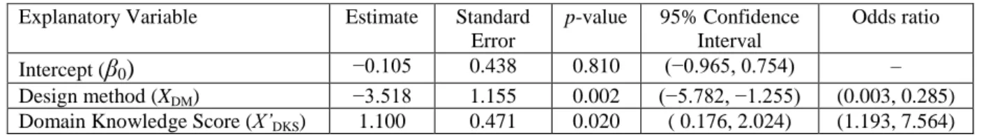
The results of the regression analysis are presented in Table 8. Note that both design method, XDM, and domain

knowledge score, X’DKS, are statistically significant at a typical threshold value of α = 0.05. As a measure of the

explanatory ability of the model, we computed a coefficient of determination as recommended by Menard (2000) resulting in a value of RL2=0.39. About half of the ability of subjects to detect mistakes in simulations

can be explained by the chosen variables and somewhat more than half remains unexplained.

As one would expect, in this experiment, a higher domain knowledge is shown to be an advantage in locating the simulation mistake. However, the largest advantage comes from choice of design method. Of the two variables, design method is far more influential in the regression equation than domain knowledge score. In this model, a domain knowledge score of more than two standard deviations above the mean would be needed to compensate for the more difficult condition of using a fractional factorial design rather than an aOFAT process.

Table 8. Logistic Regression Coefficients for Subject Debriefing

Explanatory Variable Estimate Standard Error p-value 95% Confidence Interval Odds ratio Intercept (

β

)

Domain Knowledge Score (X’DKS) 1.100 0.471 0.020 ( 0.176, 2.024) (1.193, 7.564)

5. Discussion of the Results

When interpreting the results in this paper, it is important to acknowledge the limited size and scope of the investigation. This experiment employed a single engineering model, a single type of mistake in that model, and a single engineering organization. We cannot be sure the effects observed here will generalize to other tasks, other modeling domains, to other kinds of errors in models, to other groups of people, or to other

statistical DOE approaches. It is possible that the catapult simulation is exceptional in some ways and that these results would not replicate on other engineering simulations. It is also important to note that this study cannot the optimal experimental design to enable subjects to detect mistakes. This study can only reliably allow comparison of the two designs studied. Replications by other investigators are essential to assess the robustness of the phenomenon reported here. Despite these reservations, this section explores the effects assuming they will replicate and generalize.

The most salient result of this experiment is the very large effect on likelihood of subjects to report noticing the mistake in the engineering model due to the experimental design that the human subjects used. We argue that the underlying reason for the observed difference is the complexity of factor changes in the fractional factorial design 27-4 as compared to the aOFAT process. If an experimenter makes a paired comparison between two experimental outcomes, and there is just one factor change, then it is relatively easy for the subject to apply physical and engineering knowledge to assess the expected direction of the difference. If instead there are four differences in the experimental conditions, it will surely be much harder to form a firm opinion of which of the results should have a larger response. Such a prediction requires, as a minimum, estimating all four effects and then computing their sum. When all four of the factors do not influence the results in all the same direction, which occurs with probability 7/8, accurately predicting the direction of the change requires not only correct estimates of the signs of the factor effects, but also accurate assessments of relative magnitude of the effects. Forming an expectation of the sign of the difference would also, in general, require estimation of some multi-factor interactions. This is clearly much harder and also subject to greater uncertainty than simply reasoning qualitatively about the sign of a single factor‟s conditional effect.

The explanation of the data based on complexity of factor changes is reasonable only given the assumption that subjects discover the mistake in the model by making comparisons between two individual experimental observations. But there are other ways to discover the mistake in the model. In the fractional factorial design 27-4 condition, subjects were presented with estimates of the main effects of each factor based on the set of eight observations of the catapult experiment after they had all been collected. Why didn‟t subjects form an expectation for the main effect of the factor “arm material” and then challenge the result when the calculations from the data violated their prediction? There are three reasons we can hypothesize here:

1) The subjects in the fractional factorial condition formed an expectation for the main effects of the factors (including “arm material”) and experienced an emotional reaction of surprise when the main effect computed was different in sign from their expectation, but the subjects were reluctant to report this emotional response during the debrief. A reasonable hypothesis is that the fractional factorial design lends an authority to the results that are a barrier to a single engineer challenging the validity of the simulation. After all, the experimental design is intended to improve the reliability of the results and make them robust to error and avoid bias in the conclusions. Perhaps engineers are confused about what kinds of reliability the factorial design can provide.

2) The subjects in the fractional factorial condition formed an expectation for the main effects of the factors (including “arm material”) and forgot about their expectation before the main effects were presented to them. As Daniel (1973) has noted, the results from one factor at a time experiments have the benefits of immediacy. Experimenters can see and react to data as they arise. By contrast, the full meaning of factorial designs fundamentally cannot be assessed until the entire set of data are available, which generally implies a delay in the violation of expectations. A reasonable hypothesis is that this time delay and the effect of the delay on the subject‟s memory is the primary cause of the differences observed in this investigation.

3) The subjects in the fractional factorial condition find the effort involved in following the experimental design to be greater and therefore lack the additional time and energy to perceive the mistake in the simulation. If this is the reason for the reduced frequency of finding the mistake in this experiment, then the result would not generalize to experiments conducted over longer periods of time. In this experiment, the data were collected and analysed over the course of a few hours. In realistic uses of experimental design in industry, the data often emerge and are analysed over several days and weeks. In addition to the main result regarding the difference between fractional factorial designs and OFAT procedures, some other features of the data are worth discussion. In studying the data from Table 7, it is interesting to us that experienced engineers express a reaction of surprise frequently when presented with predictions from a simulation. Almost half of the reactions we analysed were rated as surprise. In viewing the video tapes, we can see instances in which engineers express surprise even when the simulation results confirm their prediction quite closely. Apparently, it is possible to be surprised that you are right about a prediction. This makes sense if you make a prediction tentatively and do not feel confident about the outcome, especially if your prediction turns out to be very accurate. The key point is that reactions of surprise are, as implemented

here, a fairly blunt instrument for research in engineering design. It would be helpful to sort reactions of surprise into finer categories. Since these different categories of surprise cannot be differentiated based on our videotapes using any techniques known to the authors, the analysis of surprise in this study can only serve as a rough indicator of the mechanisms by which engineers find mistakes in simulations.

6. Recommendations for Engineering Practice

If the results of this study are confirmed and can generalize to a broad range of engineering scenarios, there will be significant implications for engineering practice. Engineers frequently view the processes of verification and validation of engineering models and the use of those models for design as separate. But engineering models are never fully validated for the full range of uses in engineering design (Hazelrigg, 1999). Mistakes in engineering models remain even when engineers feel confident enough to begin using them to make decisions. The results in this paper clearly indicate that more steps should be taken to ensure that mistakes in simulations will continue to be detected and reported during the subsequent steps of the design process.

Two different approaches to exercising engineering models were considered in this study and these two are traditionally used for different purposes. The fractional factorial design considered here is most often used for estimation of main effects, is frequently used as an early step in response surface methodology, and is also used within Taguchi methods as a means for reducing sensitivity of the engineering response to the effects of noise factors. The adaptive One Factor at a Time approach was proposed for use in improvement of an engineering response and was subsequently adapted as an alternative to Taguchi methods for robustness improvement. The relevant criterion in this study is to detect mistakes in an engineering model. The aOFAT approach does better than the fractional factorial design for this purpose, but neither was originally developed for this goal. A more general question is what sorts of designs are good for their intended purposes and also able to strongly support the engineers‟ ability to critically evaluate the results. The answer suggested by this manuscript is that complex factor changes are strongly detrimental to the process of mistake detection.

One remedy we argue for strongly is that the complexity of factor changes should be limited during the design process, at least for some samples of paired comparisons. If an engineer cannot anticipate any of the relative outcomes of a model in a set of runs, then we strongly encourage the engineers to make at least a few comparisons simple enough to understand fully. The engineer should choose a baseline case that is well understood and then find a comparator for which the factor changes will be simplified until the engineer can form a strong expectation about the relative change. Such simple comparisons for use in spot checking are readily available within full factorial designs and central composite designs. In Design of Computer Experiments, such as Latin Hypercube Sampling, there are no simple factor changes among any pairs of results. However, some paired comparisons can be found that approximate a change in a single factor and these might be used to spot check for mistakes in the simulations. Alternately, additional samples might be created that enforce simplicity in the factor changes so that spot checks can be made. In any case, the need for diligence in discovery of mistakes in engineering models is strongly emphasized by the results of this study. It is hoped that the data in this paper serve as a means to raise awareness of the frequency and severity of mistakes in simulations and the challenges of perceiving those mistakes. The increased awareness of these issues, by itself, would be a valuable outcome of this research.

We wish to emphasize in discussing the implications of the data presented here that the concerns about mistake detection in engineering may apply as strongly to use of physical models as they do to computer simulations. Mistakes can and frequently do occur when we run a physical experiment to make a prediction. The physical system used in an experiment is rarely exactly the same as the referent about which the predictions are being made. Further, in the conduct of an experiment by humans, mistakes can be made setting the values of experimental factors, labelling of materials and components, recording observations, and so on. It should be clear for example that in the specific case of the catapult data presented to the human subjects in this experiment, we could have presented data from a physical experiment in which the identity of the two physical items were confused (the aluminium and the magnesium catapult arms). The outcomes would be very similar to those when we instead entered the density data in the wrong fields of a computer code. We therefore emphasize that the need for simplification of factor changes may apply as much to design of physical experiments as to computer experiments.