HAL Id: tel-00811505
https://tel.archives-ouvertes.fr/tel-00811505
Submitted on 10 Apr 2013
HAL is a multi-disciplinary open access archive for the deposit and dissemination of sci-entific research documents, whether they are pub-lished or not. The documents may come from teaching and research institutions in France or abroad, or from public or private research centers.
L’archive ouverte pluridisciplinaire HAL, est destinée au dépôt et à la diffusion de documents scientifiques de niveau recherche, publiés ou non, émanant des établissements d’enseignement et de recherche français ou étrangers, des laboratoires publics ou privés.
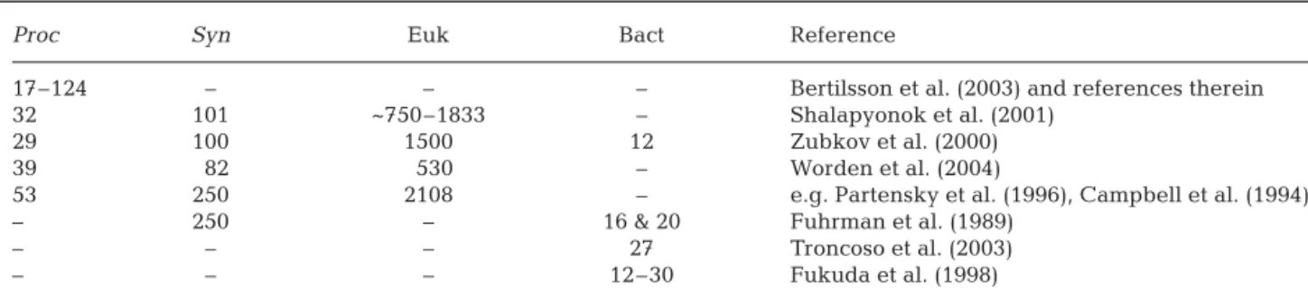
picoplanktonic carbon biomass and to total particulate
organic carbon in the open ocean.
Carolina Grob
To cite this version:
Carolina Grob. Contribution of photosynthetic picoeukaryotes to the picoplanktonic carbon biomass and to total particulate organic carbon in the open ocean.. Ocean, Atmosphere. Université Pierre et Marie Curie - Paris VI, 2007. English. �NNT : 2007PA066217�. �tel-00811505�
T
HESE DED
OCTORAT DE L’U
NIVERSITEP
IERRE ETM
ARIEC
URIE(P
ARISVI)
LABORATOIRE D’OCEANOGRAPHIE DE VILLEFRANCHE
Présentée par
Carolina Grob
Pour obtenir le grade de
DOCTEUR de l’UNIVERSITÉ PIERRE ET MARIE CURIE
Sujet de la thèse :
Contribution des picoeucaryotes
photosynthétiques à la biomasse
picoplanctonique et au carbone organique
particulaire total dans l’océan ouvert
soutenue le : 14 Mai 2007 devant le Jury composé de :
Mme Vivian Lutz Docteur Rapporteur
Mr Josep Gasol Docteur Rapporteur
Mme Carmen Morales Professeur Examinateur
Mr William K. W. Li Docteur Examinateur
Mr Alain Saliot Professeur Examinateur
Mr Hervé Claustre Directeur de recherches CNRS Co-directeur de thèse Mr Osvaldo Ulloa Professeur Co-directeur de thèse
Dedicated to my family. Dedicado a mi familia. Dediée à ma famille.
ACKNOWLEDGMENTS
First of all I would like to thank fate for sitting Dr. Ricardo Galleguillos and Dr. Osvaldo Ulloa side by side on a Concepción-Santiago flight back in 2002. I had just finished my undergraduate degree and Osvaldo was looking for someone to work with him on Prochlorococcus cell cycle. Dr. Galleguillos told him that I was looking for a job and after a short interview Osvaldo hired me for 6 months. Those 6 months made me realize that I really liked Oceanography and I started my Ph. D. in 2003.
I would like to thank all the organisms that provided me with financial support during my thesis: the Chilean National Commission for Scientific and Technological Research (CONICYT) through the FONDAP Program and a graduate fellowship; the French-Chilean ECOS (Evaluation and Orientation of the Scientific Cooperation)-CONICYT program, the French program PROOF (Processus Biogeochimiques dans l’Océan et Flux), Fundación Andes and the Observatoire Oceanologique of Villefranche (OOV). I am specially grateful to Dr. Osvaldo Ulloa and Dr. Hervé Claustre for receiving me in their laboratories, for giving me the chance to participate in the BIOSOPE cruise and for guiding me in the best way during my thesis and leaving me at the same time the autonomy necessary to accomplish this wonderful experience. It is Dr. Oscar Pizarro that I have to thank for including me in his ECOS-CONICYT project that allowed me to do my thesis in co-tutoring between Chile and France.
I would like to sincerely thank all the scientists that have inspired and motivated me and whose advices were very enriching. I would also like to thank all the technicians, engineers and crew members, without whom I could not have done this. To all my friends from Villefranche and Concepción thank you very much for all the moments shared and specially for all the good beers drunk regardless of the day of the week. Finally I would like to thank my family (my father and mother, Géraldine, Vanessa, Cotín and Boris) for all their patience, comprehension and unconditional support.
AGRADECIMIENTOS
Primero que nada quisiera agradecer al destino por haber sentado a los Drs. Ricardo Galleguillos y Osvaldo Ulloa juntos en un vuelo Concepción-Santiago en el 2002. Recién había terminado mi tesis de pregrado y Osvaldo andaba buscando a alguien para trabajar con él en el ciclo celular de Prochlorococcus. El Dr. Galleguillos le dijo que yo estaba buscando trabajo, tras lo cual Osvaldo me entrevistó y contrató finalmente por 6 meses. Esos 6 meses me ayudaron a darme cuenta que en realidad me gustaba mucho la Oceanografía y es por eso que empecé mi doctorado en el 2003.
Agradezco a todos los organismos que me financiaron durante la realización de esta tesis: Comisión Nacional de Investigación Científica y Tecnológica (CONICYT), a través del programa FONDAP y una beca de postgrado; el programa franco-chileno ECOS (Evaluación y Orientación de la Cooperación Científica)-CONICYT, el programa Francés PROOF (Processus Biogeochimiques dans l’Océan et Flux), Fundación Andes y el Observatorio Oceanológico de Villefranche (OOV).
Un muy especial agradecimiento para los doctores Osvaldo Ulloa y Hervé Claustre por acogerme en sus respectivos laboratorios, por permitirme participar en el crucero BIOSOPE y por guiarme de la mejor forma posible durante esta tesis, dándome al mismo tiempo la autonomía necesaria para llevar a cabo esta maravillosa experiencia. Fue gracias al Dr. Oscar Pizarro, quién me incluyó en su proyecto ECOS-CONICYT, que pude realizar mi tesis en co-tutela entre Chile y Francia.
Por miedo de olvidar a alguien, quisiera agradecer en forma general a todos los científicos que me inspiraron y motivaron durante mi tesis y cuyos consejos fueron muy enriquecedores. Me gustaría agradecer también a todos los técnicos, ingenieros y tripulantes, sin los cuales no hubiera podido llevar esta tesis a buen término. Quisiera agradecer además a todos mis amigos de Villefranche y Concepción por todos los momentos compartidos y sobre todo por todas esas bien merecidas cervezas bebidas sin importar el día de la semana.
Finalmente quisiera agradecer a mi familia (papá, mamá, Géraldine, Vanessa, Cotín y Boris) por su paciencia, comprensión y apoyo incondicional.
REMERCIEMENTS
Le destin a voulu que MM Ricardo Galleguillos et Osvaldo Ulloa voyagent ensemble dans un vol Concepción-Santiago en 2002. Je finissais alors mes études de Biologie Marine et Osvaldo cherchait quelqu’un pour travailler avec lui sur le cycle cellulaire de
Prochlorococcus. Sur les conseils du Dr. Galleguillos et après un court entretien,
Osvaldo m’a embauché pendant 6 mois. Ce contrat m’a permis de me rendre compte que l’Océanographie me plaisait vraiment et j’ai commencé mon doctorat en 2003. Je veux remercier les organismes qui m’ont aidés financièrement pendant ma thèse: la Commission Chilienne pour la Recherche Scientifique et Technologique (CONICYT) à travers le programme FONDAP et une bourse de doctorat, le programme franco-chilien ECOS (Evaluation et Orientation pour la Coopération Scientifique)-CONICYT, le programme Français PROOF (Processus Biogeochimiques dans l’Océan et Flux), la Fondation Andes et l’Observatoire d’Océanologie de Villefranche (OOV).
Je voudrais tout particulièrement remercier MM Osvaldo Ulloa et Hervé Claustre pour m’avoir accueilli dans leur laboratoire respectives, permis de participer à la mission BIOSOPE, efficacement encadré pendant le déroulement de ma thèse tout en me laissant l’autonomie nécessaire à la réalisation de cette belle expérience. J’ajoute que c’est grâce à M. Oscar Pizarro qui m’a intégrée le projet Ecos-CONICYT qui j’ai pu réaliser ma thèse en co-tutelle entre le Chili et la France.
Par peur d’oublier quelqu’un, j’aimerais remercier sincèrement tous les scientifiques qui m’ont inspirée, motivée et dont les conseils furent pour moi très formateurs. Je voudrais remercier aussi les techniciens, ingénieurs et membres d’équipage, sans qui je n’aurais pu mener cette thèse à bien. Au-delà, j’adresse un grand merci à tous les amis de Villefranche et de Concepción pour tous les moments partagés et notamment les bonnes bières bien méritées quelque soit le jour de la semaine.
Enfin, je voudrais remercier ma famille (mon père et ma mère, Géraldine, Vanessa, Cotín et Boris) pour toute leur patience, compréhension et soutien inconditionnels.
ABSTRACT
Contribution of photosynthetic picoeukaryotes to the picoplanktonic carbon biomass and to total particulate organic carbon in the open ocean.
María Carolina Grob Varas
University of Concepción - University of Pierre and Marie Curie (Paris VI) Ph. D. program in Oceanography, 2007
Drs. Osvaldo Ulloa and Hervé Claustre, thesis co-directors
It has been known since the early eighties that picophytoplankton (<2-3 µm) constitutes an important fraction of the total photosynthetic biomass and primary production in the open ocean. Three main groups have been identified within the picophytoplankton: two cyanobacteria, i.e., Prochlorococcus and Synechococcus, and picophytoeukaryotes belonging to different taxa. Although cyanobacteria, specially Prochlorococcus, tend to dominate numerically, the picophytoeukaryotes have been shown to dominate in some cases the picophytoplanktonic biomass and production, due to their bigger size and higher intracellular carbon content.
In the present work it was hypothesized that the spatial variability in picophytoplankton (i.e., Prochlorococcus, Synechococccus and picophytoeukaryotes) carbon biomass is essentially determined by the picophytoeukaryotes and that this group contributes significantly to the diel variability in the total particulate organic carbon (POC) concentration. In order to test these hypotheses, picophytoplankton as well as bacterioplankton (i.e, Bacteria + Archaea) abundances and carbon biomasses were assessed during two different oceanographic cruises (BEAGLE and BIOSOPE) carried out across the eastern South Pacific (between Tahiti and the coast of Chile) during austral spring time. Whereas abundances were always determined through flow cytometry, biomasses were estimated using carbon conversion factors from the literature (BEAGLE) or from group-specific contributions to the total particle beam attenuation coefficient (cp), a proxy for POC (BIOSOPE).
The general tendency in picoplankton abundances and biomasses was to increase from oligo- (or hyper-oligo-) to mesotrophic conditions in the eastern South Pacific (Prochlorococcus, Synechococcus, picophytoeukaryotes and bacterioplankton reaching up to 116, 21, 7 and 860 x 1011 cells m-2, respectively), with a slight decrease towards
eutrophic conditions for all except the bacterioplankton, Prochlorococcus not being detected near the coast. Picophytoeukaryotes constituted an important fraction of the picophytoplankton (>50% in most of the studied area) and total phytoplankton carbon biomass (>20% in the open ocean), being indeed essential in determining the spatial variability of the former. However, this group’s contribution to the diel variability in the
cp-derived POC concentration was not significant (~10%). Daily rates of change (d-1) in
picophytoplankton biomass, on the other hand, presented a significant positive correlation to those in cp (r = 0.7; p < 0.001). The usefulness of cp as a proxy for
photosynthetic carbon biomass, compared to chlorophyll a, is briefly discussed.
Picophytoeukaryotes carbon biomass was much more important than previously thought, equally or more important than that of Prochlorococcus in the open ocean. This group could therefore be playing a very important ecological and biogeochemical role in subtropical gyres, which extend over a vast area of the world’s ocean.
RESUMEN
Contribución de los picoeucariontes fotosintéticos a la biomasa picoplanctónica y al carbono orgánico particulado total en el océano abierto.
María Carolina Grob Varas
Universidad de Concepción - Universidad de Pierre y Marie Curie (Paris VI) Programa de Doctorado en Oceanografía, 2007
Drs. Osvaldo Ulloa y Hervé Claustre, co-directores de tesis
El picofitoplancton (<2-3 µm) constituye una fracción importante de la biomasa fotosintética total y de la producción primaria en el océano abierto. Dentro del picofitoplancton se han identificado tres grupos principales: las cianobacterias
Prochlorococcus y Synechococcus, y picofitoeucariontes pertenecientes a distintos taxa.
Si bien las cianobacterias, especialmente Prochlorococcus, tienden a dominar en número, se ha visto que los picofitoeucariontes pueden llegar a dominar la biomasa y producción picofitoplanctónica, debido a su mayor tamaño y contenido intracelular de carbono.
El presente trabajo se realizó bajo las hipótesis que la variabilidad espacial de la biomasa picofitoplanctónica (i.e., Prochlorococcus, Synechococccus y
picofitoeucariontes) está esencialmente determinada por los picofitoeucariontes y que este grupo contribuye en forma significativa a la variabilidad diurna de la concentración del carbono orgánico particulado total (COP). Para contrastar dichas hipótesis se determinaron las abundancias y biomasas picofitoplanctónicas y bacterioplanctónicas (i.e, Bacteria + Archaea) en términos de carbono durante los cruceros oceanográficos BEAGLE y BIOSOPE realizados a través del sector este del Pacífico Sur (entre Tahiti y la costa de Chile), durante la primavera austral. En ambos casos las abundancias fueron determinadas mediante citometría de flujo, mientras que las biomasas se estimaron usando factores de conversión de la literatura (BEAGLE) o a través de las contribuciones específicas de cada grupo al coeficiente de atenuación particulado (cp),
que es un proxy de la concentración de COP (BIOSOPE).
Las abundancias y biomasas picoplanctónicas tendieron a aumentar desde condiciones oligo- (o hyper-oligo-) hasta condiciones mesotróficas en el Pacífico Sur-este (Prochlorococcus, Synechococcus, picofitoeucariontes y el bacterioplancton alcanzando
hasta 116, 21, 7 y 860 x 1011 cel m-2, respectivamente), con una leve disminución hacia condiciones eutróficas en todos los grupos excepto el bacterioplancton, sin detectarse
Prochlorococcus cerca de la costa. Los picofitoeucariontes constituyeron una fracción
importante de la biomasa picofito- (>50% en gran parte del área de estudio) y fitoplanctónica total (>20% en el océano abierto), determinando efectivamente la variabilidad espacial de la primera. La contribución de este grupo a la variabilidad diurna del COP, sin embargo, no fue significativa (~10%). Las tasas de cambio diurno (d-1) de la biomasa picofitoplanctónica, por otra parte, presentaron una correlación positiva significativa con aquellas de cp (r = 0.7; p < 0.001). Se discute brevemente la
utilidad de cp como proxy de la biomasa fotosintética, comparado con la clorofila a.
La biomasa de los picofitoeucariontes resultó ser mucho más importante de lo que se creía hasta ahora, siendo equivalente o más importante que aquella de Prochlorococcus en el océano abierto. Por lo tanto, este grupo pudiera estar jugando un rol ecológico y biogeoquímico muy importante en los giros subtropicales, que se extienden a lo largo de vastas áreas del océano mundial.
RESUME
Contribution des picoeucaryotes photosynthétiques à la biomasse picoplanctonique et au carbone organique particulaire total dans l’océan ouvert.
María Carolina Grob Varas
Université de Concepción - Université de Pierre et Marie Curie (Paris VI) Programme de Doctorat en Océanographie, 2007
MM Osvaldo Ulloa et Hervé Claustre, co-directeurs de thèse
Le picophytoplancton (diamètre <2-3 µm) constitue une fraction importante de la biomasse phytoplanctonique totale et de la production primaire dans l’océan ouvert. Parmi le picophytoplancton, trois groupes principaux ont été identifiés: les cyanobactéries Prochlorococcus et Synechococcus, et des picophytoeucaryotes appartenant à des taxa différents. Bien que les cyanobactéries, spécialement
Prochlorococcus, dominent généralement en nombre, les picophytoeucaryotes peuvent
dans certains cas dominer la biomasse et production picophytoplanctoniques, grâce à leur taille et contenu intracellulaire de carbone plus élevés.
Ce travail s’appuie sur les hypothèses que la variabilité spatiale de la biomasse picophytoplanctonique dans l’océan ouvert (i.e., Prochlorococcus, Synechococccus et picophytoeucaryotes) est essentiellement déterminée par les picophytoeucaryotes et que ce groupe contribue significativement à la variabilité journalière de la concentration du carbone organique particulaire total (COP). Pour tester ces hypothèses, les abondances du picophytoplancton, ainsi que celles du bacterioplancton (i.e, Bacteria + Archaea) ont été déterminées lors de deux campagnes océanographiques dans le Pacifique Sud Est entre Tahiti et la côte chilienne (BEAGLE et BIOSOPE). Dans les deux cas les abondances ont été déterminées par cytométrie en flux, alors que les biomasses en carbone ont été estimées en utilisant des facteurs de conversion tirés de la littérature (BEAGLE) ou à travers les contributions des différents groupes planctoniques au coefficient d’atténuation particulaire (cp), un proxy de la concentration de COP
(BIOSOPE).
La tendance générale est une augmentation des abondances et biomasses picoplanctoniques entre les conditions oligo- (ou hyper-oligo) et mesotrophiques dans le Pacifique Sud Est (Prochlorococcus, Synechococcus, picophytoeucaryotes et
bacterioplancton atteignant jusqu’à 116, 21, 7 et 860 x 1011 cel m-2, respectivement), avec une légère diminution vers les eaux eutrophiques côtières pour tous sauf le bacterioplancton, les Prochlorococcus n’ayant pas été détectés sur la côte. Les picophytoeucaryotes représentaient une fraction importante de la biomasse picophytoplanctonique (>50% dans la plupart de la zone d’étude) et phytoplanctonique totale (>20% dans l’océan ouvert), déterminant la variabilité spatiale de la première. De plus, la contribution de ce groupe à la variabilité journalière de la concentration de COP n’était pas significative (~10%). Les taux de changement journaliers de cp (d-1), d’une
autre parte, étaient significativement corrélés à ceux de la biomasse picophytoplanctonique (r = 0.7; p < 0.001). L’utilité de cp comme proxy de la biomasse
picophytoplanctonique est brièvement discutée par rapport à celle de la chlorophylle a. La biomasse des picophytoeucaryotes était beaucoup plus importante de ce qui était initialement anticipé, étant souvent plus importants que celle des Prochlorococcus dans l’océan ouvert. Les picophytoeucaryotes jouerait donc un rôle écologique et biogéochimique dominant dans les gyres subtropicaux, lesquelles occupent une vaste superficie de l’océan mondial.
TABLE OF CONTENTS
Figures ... i
List of abbreviations ... vi
1. General introduction... 1
1.1 Picoplankton group-specific abundances, biomasses and contributions to total particle beam attenuation coefficient (cp)... 4
2. Methods ... 11
2.1 Flow cytometry... 12
2.1.1 Picoplankton abundance... 13
2.1.2 High-DNA (HDNA) and low-DNA (LDNA) containing bacteria... 14
2.1.3 Mean normalized forward scatter signal ... 15
2.2 Mean picoplankton cell size ... 16
2.2.1 Isolating picoplankton populations: FACSAria cell sorting... 16
2.2.2 Determining actual mean cell size: Coulter Counter measurements... 17
2.3 Estimating particulate organic carbon concentration (POC, mg m-3) from the particle beam attenuation coefficient (m-1)... 17
2.3.1 Group-specific attenuation coefficients resolving the different particle contributors to cp... 19
2.4 Picophytoplankton carbon biomass ... 21
2.5 Temporal variability ... 22
2.5.1 Diel cycle... 22
2.5.2 Daily rates of change ... 22
3. Picoplankton abundance and biomass across the eastern South Pacific Ocean along latitude 32.5ºS... 24
4. Contribution of picoplankton to the total particulate organic carbon (POC)
concentration in the eastern South Pacific... 27
5. Discussion and conclusions... 30
5.1 Picoplankton abundances and distribution ... 32
5.2 Picoplankton carbon biomasses and contributions to total particulate organic carbon (POC)... 36
5.2.1 Spatial variability in group-specific contributions to total particulate organic carbon (POC)... 39
5.2.2 Temporal variability ... 41
5.3 Significance of the thesis results in a global context... 45
5.3.1 Implications for global marine primary production ... 45
5.3.2 Implications for open-ocean carbon export ... 47
5.3.3 Picophytoeukaryotes role under changing environmental conditions.... 48
6. Perspectives ... 52
Literature cited... 55
FIGURES
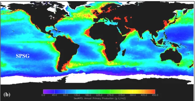
Fig. 1. (a) Global, annual average net primary productivity on land and in the ocean during 2002 (kgC m-2 y-1). The yellow and red areas show the highest rates (2-3 kgC m-2 y-1), whereas the green, blue, and purple shades show progressively lower productivity. Downloaded from http://earthobservatory.nasa.gov/Newsroom/NPP/npp.html. (b) Global, annual average marine primary production between September 1997 and August 1998 (gC m-2). Downloaded from http://marine.rutgers.edu/opp/swf/ Production/results. SPSG stands for South Pacific Subtropical Gyre.
Fig. 2. Distribution of different planktonic groups according to their size fraction. Although in this figure picoplankton is defined to be between 0.2 and 2 µm, the upper limit has also been defined at 3µm. Modified from Sieburth et al. (1978).
Fig. 3. Electronic microscopy images of Prochlorococcus (a, scale bar is 5 µm),
Synechococcus (b, same scale as a) and Micromonas pusilla (c), one of the most
common picophytoeukaryotic cells found in the coastal ocean (1 to 3 µm). Cyanobacteria images were downloaded from www.sb-roscoff.fr/Phyto/gallery and M.
pusilla from www.smhi.se/oceanografi/oce_info_data/plankton_checklist.
Fig. 4. Surface chlorophyll a concentrations estimated from satellite and in situ. Red dots indicate the geographical location of the stations where surface chlorophyll a was measured in situ. Note that the lowest estimated concentrations are observed in the South Pacific Subtropical Gyre (SPSG). From Maritorena, pers. comm.
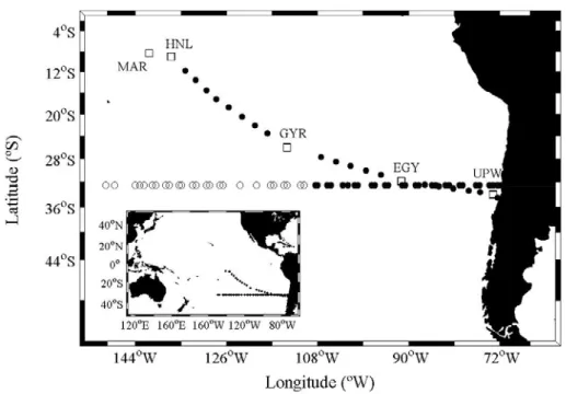
Fig. 5. The data used in the present work was obtained during two different oceanographic cruises: (1) BEAGLE (Blue Earth Global Expedition, JAMSTEC; Uchida & Fukasawa 2005) and (2) BIOSOPE (BIogeochemistry & Optics SOuth Pacific Experiment). Empty and filled circles along 32.5ºS indicate the locations where surface and water column samples were taken during the BEAGLE cruise, respectively. Squares indicate the locations of stations sampled at high frequency (every 3h; MAR, HNL, GYR, EGY and UPW) during the BIOSOPE cruise. Filled circles between these long stations indicate the location of the stations sampled at local noon time during BIOSOPE.
Fig. 6. Schematic diagram of a flow cell. During picophytoplankton analyses, samples enter the flow cytometer through this compartment, where cells are aligned thanks to the laminar flow assured by the sheath fluid. Once they are aligned, cells pass one by one in front of the laser beam. Downloaded from http://biology.berkeley.edu/crl/ flow_cytometry_basic.html.
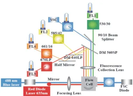
Fig. 7. Schematic diagram of the internal structure of a flow cytometer, including the flow cell. After being hit by the blue laser beam, the signals that can be recovered from the cells in the sample are forward light scatter (FSC), side scatter (SSC), yellow-green fluorescence (FL1, usually from the dies used to stain bacterioplankton cells), orange fluorescence (FL2, from Synechococcus ficoerythrin for instance), red fluorescence (FL3, from chlorophyll a, mono- as well as divinyl). Additional signals can be retrieved when using flow cytometers equipped with a second (red) laser (e.g., FL4).
Fig. 8. Example of cytograms. (a) Picophytoplankton populations (Prochlorococcus,
Synechococcus and picophytoeukaryotes) are differentiated based on their forward
scatter (FSC) and chlorophyll fluorescence signals. Reference beads of 1 µm are included in the sample. (b). Bacterioplankton is differentiated based on their FSC and the yellow-green fluorescence signal of the DNA dye used (SYBR-Green I). HDNA and LDNA stand for bacterioplankton with high and low DNA content, respectively.
Fig. 9. Example of bacterioplankton DNA distribution. Bacterioplankton DNA being stained with SYBR-Green I, high DNA (HDNA) and low DNA (LDNA)-containing bacterioplankton can be identified in the yellow-green (FL1) signal distribution of this die. Bottom vertical arrow indicates the approximate limit between HDNA and LDNA-containing bacteriopalnkton populations.
Fig. 10. Example of forward light scatter cytometric signal (FSC) distribution for reference beads (a) and picophytoeukaryotes (b). Mean FSC for beads were obtained by fitting a Gaussian curve (dark line in (a)), whereas for picophytoeukaryotes we used the whole signal’s distribution, except for the outliers observed at both ends of the distribution that have already been removed from this figure (b). Note that 3 different picophytoeukaryotes peaks, each one of them probably corresponding to a different population, can be clearly identified from this group’s FSC distribution (b).
Fig. 11. Schematic diagram of the stream-in-air droplet principle used by the fast cell sorting system of the FACSAria flow cytometer. The identified cells of interest are first charged with the charging electrode and then deflected by the deflection plates according to the charge that has been given to them. These cells are ultimately collected in different collection tubes.
Fig. 12. Example of the Coulter Counter’s particle size distribution for a picophytoeukaryotes population isolated in situ using fast cell sorting. Both the original size distribution (light line) and the data used to calculate the arithmetic mean of the identified picophytoeukaryotes population (dark line) are shown.
Fig. 13. Simplified scheme of light attenuation by a particle. The incident light is attenuated through absorption and scattering by that particle.
Fig. 14. Relationship between particle attenuation (cp) and particulate organic carbon
(POC). The solid circles, the linear fit (continuous line), and the equation correspond to measurements performed at 5ºS, 150ºW. The open circles correspond to values derived from a power law model linking cp to POC (Loisel & Morel, 1998) fitted to a linear
relationship (POC = 506.71 cp + 2.32 and r2 = 0.99) shown as the dashed line. Extracted
from Claustre et al. (1999).
Fig. 15. Example of volume distribution of particles in terms of µm3 ml-1 per 1 µm obtained using a HIAC particle counter. A peak assumed to correspond to a large phytoplankton group (>3 µm) is observed around 5 µm. Vertical dashed lines indicate the beginning and end of the identified peak and the diagonal arrow shows the approximate (App.) location of the logarithmic base line for the volume distribution of particles. Only the data within these limits was considered to calculate the average size for this group, as its arithmetic mean. The number of particles within the same limits was taken as cell abundance for the identified phytoplankton group.
Fig. 16. Example of a hypothetical data set from 40 m depth for which the daily rate of change was calculated. Each dot corresponds to a different sample. Samples were taken every 3h during 2 to 4 days. A regression line was fitted to the whole data set. The slope of this regression line (black line) was then normalized to the average value for the whole data set. Finally, the normalized slope was standardized to 24h to obtain a daily rate of change (d-1).
Fig. 17. Schematic representation of the log-log relationships between mean cell size and abundance (a) and between mean cell size and carbon biomass (b) expected from ecological theory.
Fig. 18. Water-columned integrated Prochlorococcus (a), Synechococcus (b), picophytoeukaryotes (c) and bacterioplankton abundances (x 1011 cells m-2) estimated during both cruises. Although during the BEAGLE cruise the data was integrated between the surface and 200 m, the abundances registered below 200 m were negligible enough for these results to be comparable to those integrated between the surface and 1.5 Ze during BIOSOPE.
Fig. 19. Picophytoeukaryotes (a) and Prochlorococcus (b) general increasing trends observed at 160-170 m (solid lines) as a response to an increase in light availability during the 4 days of sampling at GYR station. The slightly negative (a) and almost negligible (b) trends observed at 190 m (dashed lines) are presented to highlight the increases observed at 160-170 m.
Fig. 20. Surface irradiance (mmole quanta m-2 s-1) the day before arriving to GYR station (Fri, Friday 11th) and during the 4 days of sampling at this station (Monday 12th to Wednesday 16th), November 2003. From Claustre, pers. comm.
Fig. 21. Water-column integrated picophytoeukaryotes carbon biomasses estimated across the eastern South Pacific. In order to compare the data from both cruises, original BEAGLE data were divided by 2, according to the mean picophytoeukaryotes intracellular carbon content estimated during BIOSOPE. The latter was 2 times lower than the conversion factors from the literature used during the BEAGLE cruise. O, M and E (top of the figure panel) stand for oligo-, meso- and eutrophic conditions.
Fig. 22. Picophytoeukaryotes contribution to integrated picoplankton (filled circles and solid line) and picophytoplanktonic (empty circles and dotted line) carbon biomass (C) during the BIOSOPE (a) and BEAGLE (b) cruises. For the BIOSOPE cruise (a), picophytoeukaryotes contribution to total phytoplankton carbon biomass (dashed line) is also presented. Note that BEAGLE integrated data starts at 110ºW, whereas that of BIOSOPE begins at 142ºW.
Fig. 23. Total particle beam attenuation coefficient (cp) ratios to the vegetal
attenuation coefficient (cnveg). Notice the much higher variability in the cp to cveg ratio.
Data from the BIOSOPE cruise.
Fig. 24. Mean diel cycles of picophytoeukaryotes abundance in cells ml-1 (a) and attenuation cross-section (σc) in x 1012 m2 cell-1 (b) between the surface and 60 m, at
MAR station. The average and standard deviation (vertical lines) values for each sampling time (i.e., 3, 6, 9, 12, 15, 18, 21 and 24 h) were obtained using the data collected during the 2 sampling days. σc for each time of the day were obtained as
indicated in Chapter 2.3.1.
Fig. 25. Mean diel cycle of integrated (0 to 1.5 Ze) particle beam attenuation (cp) at
MAR station. Vertical lines indicate the standard deviations for each sampling time. Fig. 26. Relationship between daily rates of change (d-1) in Prochlorococcus (Proc),
Synechococcus (Syn) and picophytoeukaryotes (Euk) carbon biomass and daily rates of
change of total particle attenuation (cp) (a) and cytometric chlorophyll fluorescence
(FL3) (b). In (a), the correlation coefficient (r) was calculated for the mean rates of change (considering all Proc, Syn and Euk biomasses rates of change) and cp. In (b), n.
s. stands for not significant.
Fig. 27. Daily rates of change (d-1) of Prochlorococcus (Proc) and Synechococcus (Syn) abundances (abund), total particle beam attenuation coefficient (Total cp) and
picophytoeukaryotes attenuation coefficient (ceuk) at MAR (a), HNL (b), GYR (c) and
EGY (d). In the case of cyanobacteria, daily rates of change in abundance are representative of daily rates of change in their attenuation coefficients, because the latter were estimated using an average cell size (see Chapter 2.3.1).
Fig. 28. The picoplankton food web: This oceanic food web based on picoplankton shows the paths of organic carbon flux determined by Richardson and Jackson. On the left is the classical “microbial loop” (gray). The two red boxes (large zooplankton and particulate organic detritus) are two carbon pools that, according to Richardson and Jackson, receive substantial export of picoplankton carbon. This new information suggests that the role of picoplankton in carbon export and fish production needs further investigation in both observations and models. Modified from Barber, 2007.
LIST OF ABBREVIATIONS PP : primary production
FSC: flow cytometric forward light scatter signal normalized to reference beads and
expressed in relative units
Picophytoplankton: includes photosynthetic cyanobacteria (Prochlorococcus and
Synechococcus) and picophytoeukaryotes
Picophytoeukaryotes: photosynthetic eukaryotic organisms ≤ 3 µm Bacterioplankton: includes all Bacteria and Archaea
Picoplankton: includes picophytoplankton and bacterioplankton Tchla: total chlorophyll a (monodivinyl + divinyl chlorophyll a) POC: total particulate organic carbon
DOC: total dissolved organic carbon
cp: total particle beam attenuation coefficient (m-1)
cveg: part of the total particle beam attenuation coefficient due to vegetal particles (pico-
and larger phytoplankton cells)
cnveg: part of the total particle beam attenuation coefficient due to non-vegetal particles (bacterioplankton, heterotrophic protists and detritus)
cproc: Prochlorococcus-specific attenuation coefficient
csyn: Synechococcus-specific attenuation coefficient
ceuk: picophytoeukaryotes-specific attenuation coefficient
cbact: bacterioplankton-specific attenuation coefficient
chet: heterotrophic protists’-specific attenuation coefficient
CHAPTER 1
1. GENERAL INTRODUCTION
Nearly half of the Earth’s primary production (PP) takes place in the ocean (Field et al., 1998; Fig. 1a). Mean global marine PP is estimated in the order of 45 (Longhurst et al., 1995) to 60 Gt C y-1 (Carr et al., 2006 and references therein), 86% of which occurs in the open ocean (Chen et al., 2003). This is due primarily to its large area, since PP rates per unit area in the open ocean are much lower than in coastal regions (Fig. 1b).
In the open ocean the photosynthetic biomass is dominated by small phytoplankton cells that fall within the picoplankton size fraction (i.e., < 2-3 µm in diameter; Fig. 2). Picophytoplankton also constitutes the background photosynthetic biomass in more productive waters where most of the biomass is constituted by larger phytoplankton cells belonging to the nano- (2-3 to 20 µm) and microphytoplankton (>20 µm), such as in coastal regions (Fig. 3).
Within the picophytoplankton, three groups have been commonly differentiated: two within the cyanobacteria - the genera Prochlorococcus (Chisholm et al., 1988) and
Synechococcus (Waterbury et al., 1979) - and the other one within the
picophytoeukaryotes, which includes different phylogenetic taxa in the Eukarya domain (Fig. 3). Until now, most of the organisms included in the latter group are only known by their genetic sequences (Moon-van der Staay et al., 2001; López-García et al., 2001; Not et al., 2007).
Because cyanobacteria tend to dominate numerically in the open ocean, most picophytoplankton studies have focused on this group. It has been recognized, however, that picophytoeukaryotes can in some cases dominate the picophytoplanktonic PP (e.g., Li, 1994 & 1995; Worden et al., 2004) and also the carbon biomass in this size fraction (e.g., Zubkov et al., 2000), but the studies have been restricted in space and time. Thus, very little is still known about the diversity (e.g., Not et al., 2007), ecology and biogeochemical role of this group, which is the focus of this thesis.
Apart from the three autotrophic groups mentioned above, picoplankton also includes the bacterioplankton, conformed by Bacteria and Archaea commonly assumed to be essentially heterotrophic. The bacterioplankton is known to use between 10 and 60% of the organic matter produced during photosynthesis, mainly in the form of dissolved organic matter (DOC) (Fuhrman, 1992 and references therein). At first, this group was
believed to remineralize all of this organic matter to inorganic nutrients and CO2.
However, bacterioplankton is now known to also use this DOC for their own growth, hence fixing it into new living carbon biomass available for grazers such as flagellates and ciliates, which will in turn be consumed by larger organisms (Fuhrman, 1992 and references therein). Thus, instead of being reconverted into inorganic nutrients and CO2,
this biomass will be available for higher trophic levels and escape immediate remineralization. The role of bacterioplankton in carbon flow is therefore undoubtedly important through this microbial loop.
In coastal regions, where the photosynthetic biomass is dominated by large cells, the organic matter produced is preferentially consumed by higher trophic levels and exported to the sediments and open ocean. In the open ocean, on the other hand, most of the primary production is assumed to be locally remineralized or take part of the microbial loop in the euphotic zone, due to the small size of the autotrophic cells (e.g., Legendre & Le Fèvre, 1995 and references therein). It has been recently suggested, however, that the role of picophytoplankton in the open ocean carbon export to the deep ocean could be much more important than previously thought, and could therefore be significantly contributing to global carbon export and sequestration (Richardson & Jackson, 2007; Barber, 2007). Therefore, the role of picophytoplankton in carbon production and export in the open ocean could be much more important than previously thought and needs to be re-evaluated.
SPSG
Fig. 1. (a) Global, annual average net primary productivity on land and in the ocean during 2002 (kgC m-2
y-1). The yellow and red areas show the highest rates (2-3 kgC m-2 y-1), whereas the green, blue, and
purple shades show progressively lower productivity. Downloaded from
http://earthobservatory.nasa.gov/Newsroom/NPP/npp.html. (b) Global, annual average marine primary production between September 1997 and August 1998 (gC m-2). Downloaded from
http://marine.rutgers.edu/opp/swf/Production/results. SPSG stands for South Pacific Subtropical Gyre.
Fig. 2. Distribution of different planktonic groups according to their size fractions. Although in this figure picoplankton is defined to be between 0.2 and 2 µm, the upper limit has also been defined at 3µm.Modified from Sieburth et al. (1978).
(b)
Fig. 3. Electronic microscopy images of Prochlorococcus (a, scale bar is 5 µm), Synechococcus (b, same scale as a) and Micromonas pusilla (c), one of the most common picophytoeukaryotic cells found in the coastal ocean (1 to 3 µm). Cyanobacteria images were downloaded from www.sb-roscoff.fr/Phyto/ gallery and M. pusilla from www.smhi.se/ oceanografi/oce_info_data/plankton_checklist/others.
1.1 Picoplankton group-specific abundances, biomasses and contributions to total particle beam attenuation coefficient (cp)
Due to their very small size, it was only after the development of flow cytometry that picophytoplankton cells could be detected, differentiated (primarily among the three groups mentioned above) and counted on regular bases and at the large scale (e.g., Li & Wood, 1988 and references therein). Macroecological studies indicate that picophytoplankton abundance tends to decrease with increasing chlorophyll a concentrations and to increase with increasing stratification (usually accompanied by low nutrients) and temperature (Li, 2002). As a result, 66% of the variance in picophytoplankton abundance can be explained by temperature (the dominant factor), nitrate and chlorophyll a concentration (Li, in press). At the group-specific level, it has been shown that higher Prochlorococcus abundances are observed in more stratified waters and at temperatures above 10ºC (Partensky et al., 1999a), whereas
Synechococcus and picophytoeukaryotes are more abundant when mixing prevails (e.g.
Blanchot and Rodier, 1996; Shalapyonok et al.; 2001). Bacterioplankton abundance, on B
the other hand, is known to be directly related to chlorophyll a concentrations (e.g., Gasol & Duarte, 2000) and to dominate the total picoplankton abundance (e.g., Zubkov et al., 2000). The relationship with chlorophyll a can have a positive or negative slope, indicating bottom-up or top-down control on bacterioplankton abundance, respectively (Li et al., 2004).
Cell abundances are usually used to estimate carbon biomasses by applying volume-based carbon conversion factors (e.g., Li et al., 1992; Campbel & Vaulot, 1993; Zubkov et al. 1998). When cell volumes are not available, cell-specific conversion factors can also be used (e.g., Blanchot et al., 2001; Sherr et al., 2005). Picophytoeukaryotes are bigger in size and present a higher intracellular chlorophyll a and carbon content than
Prochlorococcus or Synechococcus (e.g., Raven, 1986 and references therein). The
above implies that lower picophytoeukaryotes abundances could reach similar or higher carbon biomasses than cyanobacteria. Furthermore, maximal growth rates per unit cell volume (1 µm3) seem to be higher for picophytoeukaryotes than for the numerically
dominant Prochlorococcus (Raven 2005 and references therein). The amount of carbon passing through the picophytoeukaryotic compartment could hence be significant in the open ocean and their role in energy and carbon flow could be much more important than previously thought. In the present thesis work I tried to determine the relevance of this group in terms of carbon biomass, not only within the picoplanktonic size fraction, but also in relation to the total particulate organic carbon.
An alternative approach to determining carbon biomasses is through the deconvolution of the total particle beam attenuation coefficient, cp, corresponding to the beam
attenuation coefficient measured at 660 nm (m-1). This coefficient has proven to be a good proxy for the concentration of total particulate organic carbon (POC, mg m-3) (e.g. Claustre et al., 1999). Vegetal as well as non-vegetal particles contribute to cp. The
contributions by the different vegetal and non-vegetal groups of particles, i.e., the group-specific contributions, can be estimated using optical theory. For this, the size, refractive index and abundance of each group needs to be known or at least assumed. Using this optically-based approach it has been estimated, for example, that in the equatorial Pacific 1-3 µm picophytoeukaryotes cells contributed with 28–46% to cp, and
therefore POC, whereas the numerically dominant Prochlorococcus represented 8-12% and Synechococcus was negligible (Chung et al., 1996; DuRand & Olson, 1996;
Claustre et al, 1999). Thus, the contribution to picophytoeukaryotes to the total particulate organic carbon in the open ocean can be considerable.
During the 24h diel (i.e., day-night) period, differences of up to 2-fold between a diurnal maximum and nocturnal minimum in cp have been observed (e.g., Chung et al., 1998;
Claustre et al., 1999). Although the non-vegetal particles tend to dominate this coefficient (e.g., Chung et al., 1998; Claustre et al., 1999; Oubelkheir et al., 2005), its diel cycle resembles that of most phytoplantkonic cells that grow and divide within 24h. Little is known, however, about the influence of the different groups that contribute to
cp on the diel variability observed in this coefficient. When assuming a constant
refractive index, group-specific attenuation coefficients are determined by size and abundance. Therefore, when assuming no diel changes in the refractive index, diel changes in group-specific attenuation coefficients are expected to be determined by changes in these two variables, resulting from growth and mortality processes. Diel variability in the cytometric forward light scatter signal (FSC), a proxy for cell size (e.g., Olson et al., 1993), and abundance have been observed in both cyanobacteria (DuRand & Olson, 1996; Binder & DuRand, 2002) and picophytoeukaryotes (Vaulot & Marie, 1999). Using the optically-based approach described above, it would therefore be possible to determine the influence of the diel variability in picoplankton-specific attenuation coefficient on that of cp. Such approach is used in the second part of this
thesis (see below).
Determining the spatial and temporal variability in the photosynthetic carbon biomass distribution among the different picophytoplanktonic groups can be useful to improve primary production estimates in the open ocean. Determining the contribution to the photosynthetic biomass by larger phytoplankton groups (nano- and microphytoplankton) towards more productive regions can help defining the limits of the area within which the small size fraction, and especially picophytoeukaryotes, dominate and are important for the ecology of the pelagic ecosystem. This is particularly important if we consider that the spatial variability in cp, and therefore POC,
seems to be determined by the vegetal particles (e.g., Claustre et al., 1999; Ouberkheir et al., 2005) and that the picophytoeukaryotes could be dominating this compartment in the open ocean. Complementing the above with information on the non-vegetal group’s contributions to the cp-derived POC can give an idea on the fate of the carbon being
indicate that the turn over rate of autotrophs must be faster than that of bacterioplankton to be able to keep up with their carbon demand (Fuhrman et al., 1989). Knowing the distribution of carbon biomass among the different contributors can therefore be helpful to identify the underlying biogeochemical pathways and ecosystem functioning.
Fig. 4. Surface chlorophyll a concentrations estimated from satellite and in situ. Red dots indicate the geographical location of the stations where surface chlorophyll a was measured in situ. Note that the lowest estimated concentrations are observed in the South Pacific Subtropical Gyre (SPSG). From Maritorena, pers. comm.
Picoplankton studies have been carried out in different regions of the world’s ocean except for most of the South Pacific Subtropical Gyre (SPSG). Based on the consistently low surface chlorophyll a concentrations (Fig. 4) and primary production rates (Fig. 1b) estimated from space, Claustre & Maritorena (2003) defined the SPSG as “the Earth’s largest oceanic desert”. More recently, Morel et al. (2007) have stated that the clearest waters of the world’s ocean are located at the centre of this gyre. Furthermore, SeaWiFS satellite images indicates that the poor conditions encountered at the centre of the gyre differ greatly from the typical high nutrients-low chlorophyll waters encountered at the western and equatorial borders of the gyre, and from the highly productive upwelling waters of the Chilean and Peruvian coasts. The eastern South Pacific constitutes a unique scenario for studying group-specific contributions, and particularly picophytoeukaryotes contribution to the total picophytoplanktonic carbon biomass and total particulate organic carbon (POC) across extreme trophic
conditions, including oligo- (≤ 0.1 mg m-3 of surface chlorophyll a), meso- (> 0.1 & ≤ 1 mg m-3) and eutrophic (> 1 mg m-3) areas (Antoine et al., 1996). The eastern South Pacific was therefore chosen as the study area for this work.
The main objective of the present work is:
To determine the contribution of oceanic picophytoeukaryotes to the picophytoplanktonic carbon biomass and to total particulate organic carbon (POC), and to their spatial and temporal variability in the euphotic layer of the open ocean.
Based on the background given above, the two following working hypothesis were posed:
Hypothesis 1: The spatial variability of picophytoplanktonic carbon biomass in the euphotic zone of the eastern South Pacific is essentially determined by the picophytoeukaryotes.
Hypothesis 2: The picophytoeukaryotes contribute significantly to the diel variability in
the total particulate organic carbon (POC) concentration.
The two specific objectives established to guide the present thesis work:
(1) To determine the contribution of picoeukaryotes to the picophytoplanktonic carbon
in the euphotic zone of the eastern South Pacific based on flow cytometry.
(2) To evaluate the contribution of picophytoeukaryotes to the total particle beam
attenuation coefficient (a proxy for POC) and its diel variability in the euphotic zone of oligotrophic and mesotrophic regions of the eastern South Pacific.
Organization of the thesis
The methods used during the development of this thesis are described in detail in
Chapter 2. The first part of the present work resulted in the publication of the scientific
article “Picoplankton abundance and biomass across the eastern South Pacific Ocean along latitude 32.5° S”, here included in Chapter 3. The data collected during the second part of the thesis was used in the elaboration of a new manuscript entitled “Contribution of picoplankton to the particle beam attenuation coefficient (cp) and
Chapter 4, which has already been submitted for publication. In Chapters 3 and 4, the
articles’ abstracts have also been included in Spanish and French.
Chapter 5 includes a general discussion on the results presented in the two previous
chapters. Several ideas regarding the relevance of this work at the larger spatial and temporal scale are also exposed. Finally, based on the questions rising from this thesis, some perspectives to the present work are presented in Chapter 6.
CHAPTER 2
METHODS
2. METHODS
Samples and data were collected during two oceanographic cruises across the Eastern South Pacific, during austral spring time:
(1) Leg-2 of the Japanese expedition BEAGLE (Blue Earth Global Expedition, JAMSTEC; Uchida & Fukasawa 2005), between Tahiti (~149.5º W) and the coast of Chile (~71.5º W) along 32.5ºS, from September 12th to October 12th, 2003 (Fig. 5).
(2) The French expedition BIOSOPE (BIogeochemistry & Optics SOuth Pacific Experiment), between the Marquesas Islands (~ 8.39ºS; 141.24ºW) and the coast of Chile (~ 34.55ºS; 72.39ºW), from October 26th to December 11th, 2004 (Fig. 5).
Additionally, phytoplankton cells from culture were used in laboratory work to establish direct relationships between the flow cytometric forward scatter signal (FSC) and both mean intracellular carbon content (see Chapter 2.2.3) and cell size (see Chapter 2.4.2).
Fig. 5. The data used in the present work was obtained during two different oceanographic cruises: (1) BEAGLE (Blue Earth Global Expedition, JAMSTEC; Uchida & Fukasawa 2005) and (2) BIOSOPE (BIogeochemistry & Optics SOuth Pacific Experiment). Empty and filled circles along 32.5ºS indicate the locations where surface and water column samples were taken during the BEAGLE cruise, respectively. Squares indicate the locations of stations sampled at high frequency (every 3h; MAR, HNL, GYR, EGY and UPW) during the BIOSOPE cruise. Filled circles between these long stations indicate the location of the stations sampled at local noon time during BIOSOPE.
2.1 Flow cytometry
Originally developed for clinical analyses, flow cytometry was first applied to phytoplankton analyses in the early eighties (e.g., Olson et al., 1983 & 1985). This technique allows counting cells on individual bases, i.e. one by one, and differentiate populations according to their optical properties. In brief, during flow cytometric analyses a very small volume of sea water (0.5 ml) is drawn through a thin tube into the flow cell where cells are aligned one after the other thanks to a constant laminar flow generated by the sheath fluid (Fig. 6).
One by one these cells are excited with a laser beam to record their emitted natural (from pigments) or added fluorescence (from fluorochromes; see Chapter 2.1.1) using different collectors, mirrors and filters (Fig. 7; see Marie et al., 2005 for details). Among the different fluorescence signals that can be detected are the red chlorophyll fluorescence (FL3), orange phycobilins fluorescence (FL2) and yellow-green induced bacterioplankton fluorescence (FL1) (Fig. 7). At the same time the forward (FSC) and side light scatter (SSC) signals are detected, the former being a proxy for cell size and the latter for cell complexity.
Fig. 6. Schematic diagram of a flow cell. During picophytoplankton analyses, samples enter the flow cytometer through this compartment, where cells are aligned thanks to the laminar flow assured by the sheath fluid. Once they are aligned, cells pass one by one in front of the laser beam. Downloaded from http://biology.berkeley.edu/crl/ flow_cytometry_basic.html.
Fig. 7. Schematic diagram of the internal structure of a flow cytometer, including the flow cell. After being hit by the blue laser beam, the signals that can be recovered from the cells in the sample are forward light scatter (FSC), side scatter (SSC), yellow-green fluorescence (FL1, usually from the dies used to stain bacterioplankton cells), orange fluorescence (FL2, from Synechococcus phycoerythrin for instance), red fluorescence (FL3, from chlorophyll a, mono- as well as divinyl). Additional signals can be retrieved when using flow cytometers equipped with a second (red) laser (e.g., FL4).
2.1.1 Picoplankton abundance
During the BEAGLE cruise samples for flow cytometry were taken at 25 surface stations (< 5 m) between Tahiti and Easter Island (~109º W) and at 6 different depths between the latter and the coast of Chile (surface, 10, 50, 100, 150 and 200 m). All samples were fixed on board with paraformaldehyde at 1% final concentration and quick-frozen in liquid nitrogen (see Chapter 3). During BIOSOPE, samples were taken at 6 to 14 different depths from the surface up to 300 m, the position of the deepest sampling being established according to the depth where the irradiance was reduced to 1% of its surface value. In this case picophytoplankton analyses were performed on board on fresh samples, whereas for bacterioplankton they were fixed with paraformaldehyde at 1% or glutaraldehyde at 0.1% final concentration and quick-frozen in liquid nitrogen (see Chapter 4). In both cases (i.e., BEAGLE and BIOSOPE) fixed samples were analysed on land within two months after the end of the corresponding cruise.
Prochlorococcus, Synechococcus, picophytoeukaryotes and bacterioplankton
equipped with a 488 nm blue laser. Picophytoplanktonic populations (cyanobacteria and picophytoeukaryotes) were differentiated based on their forward scatter (FSC) and chlorophyll a fluorescence (FL3) signals (Fig. 8a) according to Marie et al. (2000). Bacterioplankton samples were stained with the fluorochrome SYBR-Green I (Molecular Probes) to differentiate this population based on FSC and the yellow-green fluorescence (FL1) of this DNA dye (Fig. 8b; Marie et al., 2000). The error associated to abundances determined using flow cytometry is ≤ 5%.
Fig. 8. Example of cytograms. (a) Picophytoplankton populations (Prochlorococcus, Synechococcus and picophytoeukaryotes) are differentiated based on their forward scatter (FSC) and chlorophyll fluorescence signals. Reference beads of 1 µm are included in the sample. (b). Bacterioplankton is differentiated based on their FSC and the yellow-green fluorescence signal of the DNA dye used (SYBR-Green I). HDNA and LDNA stand for bacterioplankton with high and low DNA content, respectively.
Abundances for the weakly fluorescent surface Prochlorococcus populations were determined by fitting a Gaussian curve (see Chapter 3) or from divinyl-chlorophyll a concentrations assuming an intracellular content of 0.23 fg (see Chapter 4). Flow cytometry data acquisition was always performed with the Cell Quest Pro software (Becton Dickinson) on log mode using 256 channels (see, for example, Fig. 9) and then analysed with the Cytowin software (Vaulot, 1989).
2.1.2 High-DNA (HDNA) and low-DNA (LDNA) containing bacteria
HDNA- and LDNA-containing bacteria were differentiated based on the yellow-green (FL1) fluorescence signal of the fluorochrome added to their DNA. Higher fluorescence indicates higher DNA content. It was therefore assumed that the first and second peaks observed in the FL1 signal distribution corresponded to LDNA- and HDNA-containing bacteria, respectively (Fig. 9). Assuming a similar distribution for both populations, the
proportion of total bacterioplankton counts corresponding to HDNA- and LDNA-containing bacteria was determined by establishing a limit between these two populations (vertical arrow in Fig. 9) and counting the cells before and after this limit.
This analysis was performed only for the BEAGLE cruise data.
2.1.3 Mean normalized forward scatter signal
Fig. 10. Example of forward light scatter cytometric signal (FSC) distribution for reference beads (a) and picophytoeukaryotes (b). Mean FSC for beads were obtained by fitting a Gaussian curve (dark line in (a)), whereas for picophytoeukaryotes we used the whole signal’s distribution, except for the outliers observed at both ends of the distribution that have already been removed from this figure (b). Note that 3 different picophytoeukaryotes peaks, each one of them probably corresponding to a different population, can be clearly identified from this group’s FSC distribution (b).
Fig. 9. Example of bacterioplankton DNA distribution. Bacterioplankton DNA being stained with SYBR-Green I, high DNA (HDNA) and low DNA (LDNA)-containing bacterioplankton can be identified in the yellow-green (FL1) signal distribution of this die. Bottom vertical arrow indicates the approximate limit between HDNA and LDNA-containing bacteriopalnkton populations.
Mean forward scatter (FSC) and chlorophyll a fluorescence (FL3) signals for the reference beads were obtained by fitting a Gaussian curve to the original 256-channels signal distribution (Fig. 10a). For cyanobacteria, population size distributions represented by FSC were assumed to follow a normal distribution and the peak of such distribution was taken as the mean. Prochlorococcus and Synechococcus FSC distributions were however not always available, because the flow cytometer parameters were set to target the higher FSC signals of the bigger picophytoeukaryotic cells (remember that FSC is a proxy for cell size). In this case of picophytoeukaryotes, FSC signals were obtained by calculating the arithmetic mean of the whole signal’s distributions, except for the outliers usually observed in the first and last 5 to 10 channels of such distribution (Fig. 10b). FL3 signals for all three groups were obtained as for the picophytoeukaryotes FSC, except that in this case no outliers were observed (not shown).
2.2 Mean picoplankton cell size
2.2.1 Isolating picoplankton populations: FACSAria cell sorting
The stream-in-air droplet sorting system of the FACSAria flow cytometer allows rapid sorting of a high number of cells. The mechanism consists on creating spaced droplets containing the cells of interest and charging them electrically (positively or negatively). The charged droplet passes then trough an electrostatic field between the deflection plates, is deflected towards the plate of opposite charge and collected into the corresponding collection tube (Fig. 11). Using this
mechanism, during the BIOSOPE cruise picophytoplankton populations were isolated
in situ from fresh samples. Each population
was then analyzed with the FACSCalibur flow cytometer to obtain their mean FSC signals (see Chapter 2.1.3). Mean cell size for the
Fig. 11. Schematic diagram of the stream-in-air droplet principle used by the fast cell sorting system of the FACSAria flow cytometer. The identified cells of interest are first charged with the charging electrode and then deflected by the deflection plates according to the charge that has been given to them. These cells are ultimately collected in different collection tubes.
different isolated populations was determined using the Coulter Counter (see Chapter 2.2.2). This is the first time ever that this kind of measurement has been performed onboard on fresh populations isolated in situ.
2.2.2 Determining actual mean cell size: Coulter Counter measurements
Actual mean cell size for populations isolated in situ (see Chapter 2.2.1) and for phytoplankton cells from culture were determined using a Coulter Counter. Average population cell sizes were calculated as the arithmetical mean of the whole group’s distribution (Fig. 12). The same populations were simultaneously analysed through flow cytometry to obtain their mean normalized FSC signals (see Chapter 2.1.3). A direct relationship was then established between FSC and size using both, populations isolated in situ and culture cells (see Fig. 3a in Chapter 4). Using this relationship it was possible to estimate mean cell size for picophytoeukaryotes populations in almost every sample analyzed during the BIOSOPE cruise. In the case of cyanobacteria, their FSC signals were available in enough samples to obtain mean cell sizes representatives of the whole transect (see Chapter 4).
2.3 Estimating particulate organic carbon concentration (POC, mg m-3) from the particle beam attenuation coefficient (m-1)
The inherent optical properties of sea water (IOP’s) depend exclusively on the medium and the different substances in it (Preisendorfer, 1961). One of the main IOP’s is the light attenuation coefficient (c, m-1), which is determined by light absorption (a, m-1) and scattering (b, m-1) at any given wavelength λ (Eq. 1).
c (λ) = a (λ) + b (λ) (1)
Fig. 12. Example of the Coulter Counter’s particle size distribution for a picophytoeukaryotes population isolated in situ using fast cell sorting. Both the original size distribution (light line) and the data used to calculate the arithmetic mean of the identified picophytoeukaryotes population (dark line) are shown.
Particles (Fig. 13), water and coloured dissolved organic matter (CDOM) contribute to the beam attenuation coefficient. At 660 nm, however, attenuation due to CDOM is considered to be negligible (Bricaud et al., 1981) and a constant value can be used for water. Beam
attenuation at 660 nm can therefore be considered as representative of particle load. The total particle beam attenuation coefficient (cp) in the ocean is determined
by both vegetal and non-vegetal particles between 0.5 and 20µm (Behrenfeld & Boss, 2006 and references therein). During the BIOSOPE cruise cp profiles were obtained
using a Star transmissometer (Wet Labs, Inc.) attached to the CTD rosette. The C-Star data was treated and validated as described in Claustre et al. (1999). Total particulate organic carbon concentrations (POC, mg m-3) were estimated from cp by
using a conversion factor of 500, based on an empirical relationship established by Claustre et al. (1999) between the two variables (Fig. 14). This relationship was validated during the BIOSOPE cruise.
Fig. 14. Relationship between particle attenuation (cp) and particulate organic carbon
(POC). The solid circles, the linear fit (continuous line), and the equation correspond to measurements performed at 5ºS, 150ºW. The open circles correspond to values derived from a power law model linking cp to POC (Loisel &
Morel, 1998) fitted to a linear relationship (POC = 506.71 cp + 2.32 and r2 = 0.99) shown
as the dashed line. Extracted from Claustre et al. (1999).
Fig. 13 Simplified scheme of light attenuation by a particle. The incident light is attenuated through absorption and scattering by that particle.
2.3.1 Group-specific attenuation coefficients resolving the different particle contributors to cp
Vegetal (cveg) as well as non-vegetal (cnveg) particles contribute to the total particle beam
attenuation coefficient (Eq. 2).
cP = cveg+ cnveg (2)
Whereas Prochlorococcus (cproc), Synechococcus (csyn), picophytoeukaryotes (ceuk) and
larger phytoplankton (>3 µm, clarge) contribute to the vegetal part of the signal (Eq. 3),
cveg = cproc + csyn + ceuk + clarge (3)
bacterioplankton (cbact), heterotrophic protists (chet) and detritus (cdet = non living
particles) contribute to the non-vegetal one (Eq. 4),
cnveg = cp – cveg = cbact + chet + cdet = cbact + 2cbact + cdet = 3cbact + cdet (4)
where chet is assumed to be approximately 2cbact (Morel and Ahn, 1991). Finally, once
cveg, cbact and therefore chet are determined, cdet is obtained directly by difference (Eq. 5).
cdet = cnveg – cbact – chet = cnveg – cbact – 2cbact = cnveg – 3cbact (5)
At 660 nm, particle absorption is negligible and beam attenuation and scattering are equivalent (Loisel and Morel, 1998). Group-specific contributions to cp are therefore
equivalent to their contributions to bp. cproc, csyn, ceuk, clarge and cbact can hence be
estimated by determining the group-specific scattering coefficients,
bi (m-1) = Ni [si Qbi] = Ni σbi (6)
9 i = proc, syn, euk, large or bact.
9 Ni (cells m-3), i.e., picoplankton abundances, and mean cell sizes (through the
relationship established with FSC, see Chapter 2.2.2) were determined using flow cytometry (see Chapters 2.1.1 & 2.2.2).
9 s (m2 cell-1), i.e., the mean geometrical cross sections, were calculated from size.
9 Qbi (dimensionless), i.e., the optical efficiency factors, were computed through the anomalous diffraction approximation at 660 nm (Van de Hulst, 1957) assuming a refractive index of 1.05 for all groups (Claustre et al., 1999).
9 [si Qbi] or σbi corresponds to the scattering cross-sections (m2 cell-1).
For Prochlorococcus and Synechococcus we used mean sizes obtained from a few samples, whereas for the picophytoeukaryotes we used the mean cell size estimated for each sample (see Supp. Mat.). For samples where picophytoeukaryotes abundance was too low to determine their size we used the nearest sample’s value. For bacterioplankton we used a value of 0.5 µm, as used by Claustre et al. (1999).
In the case of larger phytoplankton (>3 µm), however, mean cell size and abundance were determined either from the Coulter Counter’s particle distribution as indicated in Chapter 2.2.2, or from the HIAC particle counter data (Royco; Pacific Scientific). When detected in the Coulter Counter particle distribution, mean cell size and abundance for large phytoplankton were determined as indicated in Chapter 2.2.2. Data collected with the HIAC were represented in the form of volume distribution of particles standardized to 1 µm (µm3 ml-1 per 1 µm). Small peaks are easier to identify using this representation (Fig. 15). In this example shown in Fig. 15, a large peak, assumed to correspond to a phytoplankton population, can clearly be seen around 4.5 and 5 µm. The average size of this population was calculated as the arithmetic mean of all data included within the identified peak, between its beginning and end, above the approximate location of the logarithmic baseline. Those data points were then added to obtain the approximate cell abundance.
Fig. 15. Example of volume distribution of particles in terms of µm3 ml-1 per 1 µm
obtained using a HIAC particle counter. A peak assumed to correspond to a large phytoplankton group (>3 µm) is observed around 5 µm. Vertical dashed lines indicate the beginning and end of the identified peak and the diagonal arrow shows the approximate (App.) location of the logarithmic base line for the volume distribution of particles. Only the data within these limits was considered to calculate the average size for this group, as its arithmetic mean. The number of particles within the same limits was taken as cell abundance for the identified phytoplankton group.