Acoustic scattering of broadband echolocation signals from prey of Blainville's beaked whales : modeling and analysis

Acoustic Scattering of Broadband Echolocation

Signals from Prey of Blainville’s Beaked Whales:

Modeling and Analysis

by

Benjamin A. Jones

B.S., United States Naval Academy, 1997

Submitted in partial fulfillment of the requirements of the degree of

Master of Science

at the

MASSACHUSETTS INSTITUTE OF TECHNOLOGY

and the

WOODS HOLE OCEANOGRAPHIC INSTITUTION

September 2006

c

° Benjamin A. Jones, 2006. All rights reserved.

The author hereby grants to MIT and WHOI permission to reproduce and distribute publicly paper and electronic copies of this thesis document in whole or in part.

Author . . . .

Joint Program in Oceanography/Applied Ocean Science and Engineering September 2006

Certified by . . . .

Andone C. Lavery, Assistant Scientist Thesis Co-Supervisor

Certified by . . . .

Timothy K. Stanton, Senior Scientist Thesis Co-Supervisor

Accepted by . . . .

Henrik Schmidt, Professor of Mechanical Engineering Chair, Joint Committee for Applied Ocean Science and Engineering

Accepted by . . . .

Lallit Anand, Professor of Mechanical Engineering Chairman, Graduate Committee

Acoustic Scattering of Broadband Echolocation Signals from

Prey of Blainville’s Beaked Whales: Modeling and Analysis

by

Benjamin A. Jones

Submitted in partial fulfillment of the requirements for the degree of Master of Science

at the Massachusetts Institute of Technology and the Woods Hole Oceanographic Institution

Abstract

Blainville’s beaked whales (Mesoplodon densirostris) use broadband, ultrasonic echolo-cation signals (27 to 57 kHz) to search for, localize, and approach prey that generally consist of mid-water and deep-water fishes and squid. Although it is well known that the spectral characteristics of broadband echoes from marine organisms are a strong function of size, shape, orientation and anatomical group, little is known as to whether or not these or other toothed whales use spectral cues in discriminating between prey and non-prey. In order to study the prey-classification process, a stereo acoustic tag was mounted on a Blainville’s beaked whale so that emitted clicks and corresponding echoes from prey could be recorded. A comparison of echoes from prey selected by the whale and those from randomly chosen scatterers suggests that the whale may have, indeed, discriminated between echoes using spectral features and target strengths. Specifically, the whale appears to have favored prey with one or more deep nulls in the echo spectra as well as ones with higher target strength.

A three-dimensional, acoustic scattering model is also developed to simulate broad-band scattering from squid, a likely prey of the beaked whale. This model applies the distorted wave Born approximation (DWBA) to a weakly-scattering, inhomoge-neous body using a combined ray trace and volume integration approach. Scatterer features are represented with volume elements that are small (less than 1/12th _{of the}

wavelength) for the frequency range of interest (0 to 120 kHz). Ranges of validity with respect to material properties and numerical considerations are explored using benchmark computations with simpler geometries such as fluid-filled spherical and cylindrical fluid shells. Modeling predictions are compared with published data from live, freely swimming squid. These results, as well as previously published studies, are used in the analysis of the echo spectra of the whale’s ensonified targets.

Thesis Co-Supervisor: Andone C. Lavery Title: Assistant Scientist

Thesis Co-Supervisor: Timothy K. Stanton Title: Senior Scientist

Acknowledgments

Nearly a decade ago as I began working in Naval aviation, I could not have imagined the wonderfully crooked path which my career would follow. The opportunity to take a two year hiatus from operational duties to pursue scientific research has fulfilled a dream. Without the advocacy of my entire chain of command, particulary CDR Michael “Reggie” Hammond and CAPT Tom Webber, and the financial support from the Office of the Oceanographer of the Navy the work here could not have been conducted.

I cannot fully express my appreciation for the support that I have received from my research advisors at the Woods Hole Oceanographic Institution. Dr. Tim Stanton, who swept me into his realm of acoustic scattering on my first day at WHOI, has a gift of enthusiasm for his work which he will bequeath on anyone fortunate enough to become involved. Dr. Andone Lavery has had the unenviable job of turning a seven year Naval officer into a nascent acoustician. I am truly grateful for her unwavering support, tireless tutoring, and always elegant way of approaching difficult problems.

The unique environment at WHOI, where barriers between research departments seem to blow away in the salty breeze, has been key to this research. My coauthors for the article on which Ch. 2 is based, biologists Dr. Peter Tyack and Dr. Peter Madsen and electrical engineer Dr. Mark Johnson, introduced me to the fascinating world of deep-diving, echolocating whales where sound illuminates the darkness. The data from the tagging of a Blainville’s Beaked whale, collected with support from Na-tional Oceanographic Partnership Program, the Office of Naval Research, and Canary Islands Government, was graciously provided by them.

The modeling section of this study could not have been completed without the energetic support of Dr. Darlene Ketten and her talented staff of technical experts, particularly Julie Arruda, R.T.(R) who conducted the CT scans of squid presented here and Sr. Research Asst. Scott Cramer who aided in the handling, transport, and preservation of the specimens. The excellent squid specimens used in this study were identified and provided by Ed Enos, Superintendent of the Aquatic Resources

Division at Marine Biological Laboratory. I would also like to mention Dr. Roger Hanlon with whom, on more than one occasion, enlightening discussions were held on the natural history of squid.

Finally, I would like to thank my spouse, Sylvie Rusay, whose endless wit and wisdom have protected my sanity through many long and often difficult academic and research hurdles. Thank you, my dear.

Contents

1 Introduction 15

1.1 Historical background on echolocation research . . . 15

1.1.1 Echolocation in bats . . . 15

1.1.2 Echolocation in toothed whales . . . 16

1.2 Broadband scattering from marine organisms . . . 18

1.3 Modeling of broadband acoustic scattering . . . 19

1.4 Overview of study . . . 21

2 Classification of broadband echoes from prey of a foraging Blainville’s beaked whale 23 2.1 Introduction . . . 23

2.2 Signals emitted by the Blainville’s beaked whale (M. densirostris) . . 24

2.2.1 FM clicks . . . 25

2.2.2 Buzz clicks . . . 26

2.3 Acoustic data acquisition . . . 26

2.3.1 Instrumentation (Digital Acoustic Recording Device, DTAG) . 26 2.3.2 Fieldwork . . . 27

2.4 Data analysis . . . 29

2.4.1 Selection criteria of echoes . . . 29

2.4.2 Spectral classification . . . 32

2.4.3 Target strength calculations . . . 33

2.5 Results . . . 36

2.5.2 Echo classification . . . 36

2.5.3 Comparison of echo characteristics between two groups of prey 41 2.5.4 Comparison between echo characteristics and scattering predic-tions/observations . . . 43

2.6 Discussion . . . 45

3 Acoustic scattering by weakly scattering shelled objects: Applica-tion to Squid 47 3.1 Introduction . . . 47

3.2 Theory . . . 49

3.2.1 Basic definitions . . . 49

3.2.2 DWBA-based scattering models . . . 51

3.2.3 Exact modal-series-based scattering models . . . 53

3.3 Materials and methods . . . 54

3.3.1 Animals studied . . . 54

3.3.2 High resolution morphometry of squid: SCT scans . . . 57

3.3.3 Numerical implementation of the DWBA ray-tracing model . . 58

3.3.4 Application to squid . . . 60

3.4 Results . . . 61

3.4.1 Scattering from fluid-filled, fluid spherical and finite cylindrical shells . . . 61

3.4.2 Application to squid . . . 68

3.5 Discussion . . . 71

4 Summary and conclusion 75 4.1 Scattering of echolocation signals . . . 75

4.2 Modeling . . . 76

4.3 Recommendations for future work . . . 76

A Modal series coefficients for fluid-filled shells 79 A.0.1 Spherical shells . . . 79 A.0.2 Cylindrical shells . . . 80 B Algorithms for DWBA ray-tracing model 81

List of Figures

2-1 Echolocation signal (FM click) of the M. densirostris . . . . 25 2-2 Echograms of scattered echolocation signals of a foraging beaked whale 28 2-3 Example of automated structure analysis. . . 32 2-4 Broadband acoustic signatures of four prey selected by the whale. . . 35 2-5 Characteristics of echo trains “selected” by the whale, and randomly

chosen “non-selected” scatterers. . . 37 2-6 Depth distribution of two groups of prey categorized by echo density. 41 2-7 Spectral content in frequency responses of “selected” prey and

“non-selected” scatterers. . . 42 2-8 Reduced target strength distribution of prey “selected” by the whale

and “non-selected” scatterers. . . 44 3-1 Diagram of the bisection of spherical shell or cross section of a

cylin-drical shell illustrating inhomogeneous material properties. . . 50 3-2 Sketches of two squid species, L. pealeii and T. pacificus. . . . 55 3-3 Volume rendering composed of SCT images of squid and four binary

cross sections. . . 56 3-4 Ray trace illustration through inhomogeneous volume. . . 58 3-5 Effect of varying shell thickness on reduced target strength for a

spher-ical, fluid-filled, fluid shell. . . 62 3-6 Effect of varying shell thickness on reduced target strength for a

3-7 Effect of varying material properties on reduced target strength for a cylindrical, fluid-filled, fluid shell of finite length. . . 65 3-8 Reduced target strength versus orientation predictions for solid

cylin-der of finite length. . . 67 3-9 Reduced target strength predictions for various tilt angles of squid

compared with published data of freely swimming and anesthetized squid. . . 69 3-10 Average reduced target strength predictions of squid . . . 70

List of Tables

2.1 Distribution of echoes from “whale-selected” and “non-whale-selected” echo trains in the three dives examined. . . 38 3.1 Material properties of squid from published sources. . . 57

Chapter 1

Introduction

1.1

Historical background on echolocation research

Echolocation is a term coined by Griffin (1944) for an animal’s emission of high frequency sounds and the consequent reception of echoes for use in obstacle avoidance. This ability, also now known to be used in hunting for prey, has been most thoroughly documented in two very distinct taxa of mammals. Most species of the suborder

Odontoceti, or toothed whales, use echolocation including members of the family Ziphiidae, or beaked whales (Johnson et al., 2004; Madsen et al., 2005; Zimmer et al.,

2005). Likewise, sound is used by the small flight-capable mammals, Chiroptera, or bats. Both of these groups of mammals have evolved echolocation capabilities for use in the absence of light. While bats use sound to navigate and hunt on the wing at night, beaked whales use echolocation to hunt for prey at ocean depths where significant sunlight cannot penetrate. A brief review of research on these animals’ biosonar, summarized in the following paragraphs, provides context for this study.

1.1.1

Echolocation in bats

Researchers have debated for over two centuries the capabilities of certain species of animals to use biosonar in orientation, communication, and prey capture. As early as 1793 Italian scientist Lazaro Spallanzani and Swiss zoologist Louis Jurine discovered

that bats depend primarily on hearing rather than sight for orientation in dark envi-ronments (Galambos, 1942). Spallanzani conducted extensive experiments in which blinded bats avoided slender obstacles, such as silk threads suspended from the ceil-ing, with the same success as visually unhindered bats. After repeating Spallanzani’s experiments on blinded bats, Jurine provided conclusive evidence that bats rely heav-ily on hearing to navigate. In a series of experiments in which bats’ ears were plugged with a variety of substances, such as wax and wood, the animals crashed aimlessly into obstacles in their path.

It was not until much later, however, with the development of G.W. Pierce’s ul-trasonic detector, that Pierce and Grifin (1938) collected data to support theories that bats use ultrasonic emissions to provide spatial orientation. Evidence of hunting minute insects using active sonar would not be found for another decade and a half (Griffin, 1953). This, in turn, has led researchers to question the extent to which bats can acoustically resolve their environment. Simmons and Vernon (1971) showed that the big brown bat (Eptesicus fuscus), using broadband frequency modulated (FM) clicks, can indeed discriminate size, shape, and distance to targets. Further-more, Siemers and Schnitzler (2000) have shown that the Natterer’s bat (Myotis

nattereri), also using FM signals, can discriminate prey from background clutter

us-ing echolocation without the aid of passive secondary cues such as prey-generated sounds or olfactory information. Bats’ use of frequency dependent cues found in echoes from objects that they ensonify is an area of ongoing research (Simmons and Chen, 1989; Schmidt, 1992; von Helversen and von Helversen, 2003). Recently, it has been suggested that bats use spectral information from sequences of target echoes to discriminate between differing shapes and sizes (von Helversen, 2004). This line of research, which gives strong evidence that bats do make use of spectral cues in object discrimination, provides motivation to explore similar adaptations in toothed whales.

1.1.2

Echolocation in toothed whales

Historically, studies on echolocation capabilities of the sub-order Odontoceti, toothed whales, have concentrated on various species of dolphins in captivity. It is well-known

that these animals transmit a variety of broadband, ultrasonic signals in order to nav-igate and hunt their prey. Many tank experiments, using artificial targets with subtle differences in size, shape and material compositions, have shown that dolphins use information contained in the broadband echoes to aid in discrimination tasks (Nachti-gall, 1980). Identifying the features of acoustic signals that dolphins use in these tasks is a goal of ongoing research. Au and Pawloski (1989) have shown that dolphins can discriminate between broadband signals having a “rippled” or “non-rippled” fre-quency spectra. Fuzessery et al. (2004), cites experiments by Vel’min and Dubrovskiy (1976), and Dubrovskiy (1989), where dolphins discriminate between pulse pairs with intervals of 0.05 to 0.2 ms, much shorter than the dolphin’s auditory integration time of 0.3 ms given by Au (1993). It is suggested that dolphins, which would perceive these pulse pairs as a single echo, may be processing them in the frequency domain. With respect to the inverse problem, research on acoustic scattering from marine or-ganisms has shown that different groups of animals can be classified by the frequency spectra of their backscattered signal (Martin et al., 1996; Stanton et al., 1998b). It is unclear, however, to what degree dolphins, or other toothed whales, use features of broadband, acoustic backscattering to aid in the classification of prey.

The limited number of in situ studies on echolocating toothed whales has limited progress in this area of research. In many species the combination of depth of the echolocating animal and attenuation of the high frequency signal prevent either ship mounted or towed sensors from recording their emitted signals. A number of recent studies, using new technologies and novel methods, have begun to advance the under-standing of these animals’ behavior in their natural environment. Using hydrophone arrays deployed from small boats to record whales foraging by echolocation (Au et al., 2004) and newly developed acoustic data tags affixed directly to echolocating whales (Johnson and Tyack, 2003; Akamatsu et al., 2005; Zimmer et al., 2005; Madsen et al., 2005) researchers have started to collect new information about the echolocation sig-nals and foraging behavior of free-ranging toothed whales. The analysis presented in Ch. 2 of this thesis is based upon data collected from such a study in which an acoustic tag recorded a beaked whale echolocating in the wild.

1.2

Broadband scattering from marine organisms

In complement to the research on the biosonar systems of these capable predators, a concurrent body of research has been conducted on acoustic scattering from marine organisms of lower trophic levels. Attempts to estimate zooplankton biomass have highlighted the need for accurate acoustic characterization of various classes of zoo-plankton (Stanton et al., 1994; Martin et al., 1996). Constructive and destructive interference of the sound wave scattered by features such as tissue interfaces or skele-ton create a frequency dependent interference pattern specific to orientation, material properties (i.e. sound speed and density), and morphology of the scatterer. Models that predict frequency specific scattering amplitude from different organisms can aid in the remote classification and identification of species being surveyed.

Recent trends in fisheries research have followed a similar course. Through the use of multibeam sonars, multiple discrete frequencies, and higher bandwidth systems, researchers have improved spatial resolution of fish schools and species identification during acoustic surveys (Horne, 2000). Broadband acoustic systems have been used with a variety of processing techniques in efforts to conduct reliable species recog-nition based on the spectral signature of backscatter from fish aggregations (Sim-monds et al., 1996; Zakharia et al., 1996). Broadband scattering from individual, swimbladder-bearing fish has also been investigated. Reeder et al. (2004) has shown that high frequency acoustic backscatter from alewife is highly frequency dependent as well as strongly affected by orientation. Combining this insightful research on scattering from marine organisms with the knowledge that echolocating whales use broadband, ultrasonic biosonars leads to the hypothesis that an acoustic basis for prey discrimination exists in the frequency dependent characteristics of the prey echoes. It is the goal of this study to elucidate specific characteristics found in prey echoes of a free-ranging beaked whale that may be used by the whale to discriminate between prey and non-prey scatterers in the water column.

1.3

Modeling of broadband acoustic scattering

Modeling of acoustic scattering from individual marine organisms complements labo-ratory and field measurements by helping to quantify factors that influence the scat-tering of sound. Furthermore, extracting biologically important information, such as species type and abundance, from high-frequency, acoustic scattering data relies heavily on the availability of experimentally validated scattering models (see review by Horne (2000)). The intended application of a model often dictates the level of complexity used in representing a marine organism as a scatterer. These applica-tions range from predicapplica-tions of volume scattering, which may use discrete scattering predictions averaged over a range of parameters such as size and orientation of the scatterer, to models that attempt to replicate discrete echoes for unique identification of class, size, or even species of scattering organism.

In general acoustic scattering from individual marine organisms is a complex process that is dependent on the frequency of the incident sound wave, the orien-tation of the scatterer with respect to the incident wave, and the size, morphology, and material properties (i.e. density and sound speed) of the organism. Scattering by organisms of widely varied anatomical groups have been modeled. Fish, both swimbladder-bearing and non-swimbladder-bearing, have been extensively modeled for use with acoustic survey data to estimate fish stocks (see reviews by Maclen-nan and Simmonds (1992); Foote (1997)). Zooplankton models have, likewise, been developed for use with echo sounder surveys. The diversity of organisms within zoo-plankton populations is reflected in the variety of models developed (see review by Foote and Stanton (2000)).

One group of zooplankton that researchers have focused on are weakly-scattering organisms with fluid-like material properties (i.e. tissue that does not support shear waves). Many advances have been made in developing high frequency acoustic scat-tering models for this group of organisms involving shapes of varying complexity. The representation of shape in early studies were based on fluid models of simple geometric volumes such as spheres, finite cylinders, and prolate spheroids (Anderson,

1950; Yeh, 1967; Johnson, 1977; Stanton, 1988). More recent models have incorpo-rated high resolution 2-D (Stanton et al., 1998a; McGehee et al., 1998; Amakasu and Furusawa, 2006) and 3-D (Lavery et al., 2002) details of zooplankton shape. The complex representation of shape in these models are made possible by the application of the distorted wave Born approximation (DWBA). This modification to the Born approximation (BA), a volume integral formulation for weakly scattering bodies, can account for complex 3-D shape as well as inhomogeneous material properties. The DWBA formulation has been successfully applied to model the scattering of sound from various types of zooplankton including euphausiids, copepods, krill and decapod shrimp and validated through field measurements (Wiebe et al., 1997; Lawson et al., 2004).

Incorporation of high resolution material properties into DWBA models such that variations correspond to the anatomical structure of the organism being simulated is still a challenge. Limited information on sound speed and density of different tissues within marine organisms, as well as difficulties in implementing the DWBA for in-homogeneous bodies, are the primary obstacles. Application of the DWBA has been primarily limited to scattering bodies of homogeneous material properties (Stanton

et al., 1993; Chu et al., 1993; Stanton et al., 1998a; McGehee et al., 1998; Stanton

and Chu, 2000; Lavery et al., 2002). Yet, marine organisms have complex internal morphologies, which include internal organs (e.g. lungs, liver, gonads, etc.), and may also include large seawater filled cavities as found in squid or jellyfish. These inter-nal structures of differing material properties create multiple interfaces that strongly affect the scattering of sound. The DWBA has been applied to inhomogeneous vol-umes by varying material properties along the length of an organism’s body (Stanton

et al., 1998a; Stanton and Chu, 2000; Lavery et al., 2002). In these cases variation

corresponded to general body composition such as segmentation of the exoskeleton. To date, however, 3-D inhomogeneities due to internal structure of an organism’s body have not been incorporated into a DWBA model. The modeling section of this thesis presents a DWBA model that can accurately account for 3-D inhomogeneities within a weakly-scattering body. This model is applied to squid, a common prey of

beaked whales, using high resolution morphology obtained from spiral computerized tomography (SCT) scans. Results from this modeling is used in the analysis of beaked whale prey discussed in Ch. 1.

1.4

Overview of study

This thesis is organized as follows. Chapter 2 presents an analysis of broadband echoes, recorded in-situ, from prey of an echolocating beaked whale. Chapter 3 reports on the development of an advanced model for weakly scattering bodies that incorporates both detailed, 3-D shape and 3-D material property inhomogeneities of the scatterer. Chapter 4 contains concluding remarks and contributions of this paper to the scientific community. Coefficients of the modal-series-based solutions for fluid shells and the algorithms used in the numerical scattering model are given in the appendices.

Chapter 2

Classification of broadband echoes

from prey of a foraging Blainville’s

beaked whale

1

2.1

Introduction

In a recent study non-invasive digital acoustic recording devices, DTAGs (Johnson and Tyack, 2003), were attached to a Blainville’s beaked whale, (Mesoplodon densirostris) and used to record echolocation signals during deep foraging dives (Johnson et al., 2004). These whales use broadband signals to search for and localize prey consisting of mesopelagic fishes and squid (Pauly et al., 1998). Acoustic data recorded by the DTAG contained both the whale’s emitted signals as well as echoes from prey in the water column. These data show that, although the whale ensonified a large number of scatterers, it only actively pursued a small percentage of them. This suggests that the animal is actively selecting certain types of prey (Madsen et al., 2005). In this paper, these data are examined to determine if there is evidence of an acoustic basis for target discrimination based on the scattering of their echolocation signals. Singly resolvable echoes from prey selected by the whale and from

non-1_{This chapter is based on an article to be submitted to the Journal of the Acoustical Society of}

selected scatterers in the water column are compared using spectral characteristics and relative target strengths. Secondly, two populations of depth separated prey are juxtaposed to provide a comparison of two, likely different prey types. Finally, the results are discussed in context with experimental and modeling results of scattering from marine organisms.

Conducting an analysis of echoes, recorded in situ, using the whale’s biosonar as a sound source and the animal’s body as the platform for the receiver present a myriad of difficulties. These challenges and how they are addressed, which are discussed in detail in the following sections, are summarized: 1) It was not feasible to make far field measurements of the sounds emitted by the whale. Instead, as a reference for the frequency responses of the scatterers, the featureless portion of the frequency spectrum of an echolocation signal recorded from another whale of the same species is used. 2) The near-field recording of the whale’s emitted signal is used as a proxy for changes in the amplitude of the emitted signal. Thus, relative target strengths of the scatterers can be obtained. 3) The unpredictability of the platform, i.e. the whale, has a significant effect on the position of the scatterer within the beam. The angle of arrival information from the hydrophone pair is used to limit, in one dimension, the position of the scatterer with respect to the longitudinal centerline of the whale. Using this carefully constrained subset of the data, it is demonstrated that there are significant differences with respect to relative target strengths and spectral content between echoes of prey selected by the whale and non-selected scatterers.

2.2

Signals emitted by the Blainville’s beaked whale

(M. densirostris)

The M. densirostris transmits two distinct echolocation signals. Johnson et al., (sub-mitted) discriminates between these signals based on their repetition rate, waveform, and frequency content. A slow repetition rate signal (referred to here as FM clicks) is used by the whale in the search and approach of prey while a high repetition rate

Figure 2-1: Echolocation signal (FM click) of M. Densirostris: (a) normalized time series, (b) frequency spectrum.

signal, called buzz clicks, is used during the terminal portion of a prey capture.

2.2.1

FM clicks

The FM clicks, following the nomenclature of Johnson et al. (submitted), are char-acterized by an upswept, frequency modulated waveform of 220 to 320 µs in length. They are produced nearly continuously at depth while the animal is searching for and localizing prey. The inter-click-interval (ICI) for the FM clicks ranges from 0.1 to 0.6 s. The associated frequency spectrum is smoothly shaped between approximately 25 to 54 kHz with a rapid fall off at lower frequencies and has -10 dB endpoints at 27 and 57 kHz (Fig. 2-1). It has been shown by Johnson et al. (submitted) that the

frequency content of these clicks, when recorded on axis, is generally consistent from ping to ping. Throughout this analysis only echoes from targets ensonified by FM clicks are considered.

2.2.2

Buzz clicks

When approaching prey to within approximately a body length, the M. densirostris switches to a high-repetition-rate click. These clicks are approximately half the du-ration of the FM clicks and are of significantly lower amplitude. This series of clicks, referred to collectively as a buzz, is often accompanied by a rapid acceleration of the whale and is believed to be associated with the final homing and capture phase of the hunt (Johnson et al., 2004). Buzzes are used in this analysis to identify the whale’s selected prey.

2.3

Acoustic data acquisition

A free-ranging beaked whale was tagged with a digital acoustic recording device, DTAG. The tag was used to record echolocation signals emitted by the whale as well as echoes from scatterers in the water column. It is the characteristics of the echoes from scatterers in the water column that are of particular interest to this study.

2.3.1

Instrumentation (Digital Acoustic Recording Device,

DTAG)

The DTAG is a small, self-contained device designed to record acoustic and orientation data from a freely swimming animal (Johnson and Tyack, 2003). This tag attaches to the surface of a whale with four suction cups, which actively release after a pre-set period of time. The version used to collect the data presented in this paper containes two hydrophones spaced 2.5 cm apart, each with a frequency response that is constant to within 3 dB between 0.4 and 67 kHz and with a sensitivity of -171 dB re V /µP a in that band. The tag samples acoustic data from each of the hydrophone channels at

a rate of 192 kHz. Also included in the tag’s sensor suite were 3-axis accelerometers are 3-axis magnetometers for orientation and a pressure sensor for extracting depth. These sensors record data at a 50 Hz sampling rate. Data are stored in a non-volatile FLASH memory array with a capacity of 6.6 gigabytes.

2.3.2

Fieldwork

An adult, female Blainville’s beaked whale (MD287a) was tagged in October of 2004, near the island of El Hierro, in the Canary Islands, by means of a 5-meter-long car-bon fiber pole from a 4-meter-long rigid-hull inflatable boat (RHIB). The animal was observed surfacing from a 7-meter-long RHIB during daylight hours, which included the acoustic portion of the recording. The tag recorded acoustic data for the prepro-grammed time of 9.5 hours. A reserve of memory allowed the logging of an additional 8.9 hours of orientation and depth data after which the tag automatically released. The tag was located and recovered with the aid of a VHF transmitter included in the tag.

The tag was initially placed on the right side of the whale, but moved to a position approximately 1 meter posterior of the blowhole on the animal’s dorsal ridge prior to the dives discussed in this paper. This position, fortuitously, minimized shading of the hydrophones by the whale’s body and provided favorable conditions for recording echoes from objects ensonified by the whale. One intrinsic difficulty with a tag located behind a whale’s head, is that only near-field, off-axis transmissions can be recorded (Johnson et al., 2004). These measurements, clearly, do not reflect actual source levels within the animal’s forward beam. However, measurements of transmitted signals from a tag in this position can provide a proxy for relative changes in the power output of the whale’s clicks (Madsen et al., 2005). Thus, it is possible to estimate ping-to-ping variation in source level.

Three dives are discussed in this paper, dives #2 - #4. During these dives FM clicks were only recorded at depths greater than 440m while the whale dove to various depths down to 1300 m. During dive #3 the whale hunted near the bottom in a narrow band of depth between 600 and 650 m as indicated by the buzzes at these depths.

Foraging during dives #2 and #4 appeared to be spread out in depth over several hundred meters; although, in both cases the majority of buzzes were concentrated in depth bands of less than 200 meters.

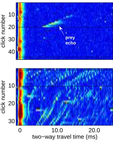
click number

two−way travel time (ms)

0

10.0

20.0

10

20

30

click number

10

20

30

40

Figure 2-2: Two representative examples of echograms displaying scattered echolo-cation signals of a foraging beaked whale which are used to identify echo trains: (a) low echo density environment, (b) high echo density environment. FM click num-ber is shown on the y-axis and the x-axis shows time since last emitted click. Echo strength is indicated by color with red corresponding to higher sound pressure and blue corresponding to lower sound pressure. The top plot shows a single echo train as the whale approaches a target. The black line represents a spacing of greater than 1 second between outgoing clicks that meet a pre-set threshold level which, in this case, indicates the whale’s switch to the lower amplitude buzz.

2.4

Data analysis

2.4.1

Selection criteria of echoes

Identifying echo trains from whale-selected prey

The acoustic data recorded by the DTAG corresponded to four full dives of this whale. Both the tagged animal’s emitted signals and scattered echoes were recorded on all four dives; however, only data from dives #2 through #4 were considered due to the preferred placement of the tag on these dives. Approximately 1.4 hours of acoustic data from these three dives were analyzed.

The acoustic record was analyzed to identify all buzzes, or suspected predation events, that occurred during the three dives of interest. Firstly, an algorithm indi-cating relative amplitude and time between clicks was used in combination with a time-frequency spectrogram of the signals to identify buzzes. Secondly, echograms were produced indicating sound power on a color scale in a plot of click number ver-sus time (see Fig. 2-2). By aligning the envelopes of the tagged whale’s transmitted clicks on one axis and two-way travel time (TWT) along the other, these echograms were used to identify echo trains, or continuous series of echoes from a single scatterer. A 25 ms TWT window was used corresponding to a range from source to scatterer of about 18 m. Using this method prey echo trains were easily identifiable by their slowly varying, and generally, monotonically decreasing TWT.

The echograms were analyzed in the vicinity of the buzzes to identify echo trains from intended prey. Only echo trains associated with regular clicks that terminated within five seconds of a buzz were selected. If multiple echo trains were identified (i.e. series of echoes with different TWT from the same outgoing transmission and, thus, different ranges from whale to scatterer) the echo train that terminated most closely to the first buzz click echo, in time, was selected. If no echo was visible from the buzz in such a case, or two echo trains were very close together in time, that sequence was not considered in the analysis. An identifiable echo from the buzz, however, was not a criterion if there was no ambiguity in selecting the echo train.

Identifying echo trains from non-selected scatterers

Randomly chosen echo trains, not selected by the whale as prey, were identified for processing on each dive. These non-selected echo trains were defined as those that did not immediately precede a buzz from the whale. The same two way travel time window of 25 ms was used to choose these non-selected echo trains.

Acoustic environment: aggregations of varying density

In addition to the discrete echoes, which were selected from the acoustic record, several other parameters were extracted from the data record such as depth and echo density. Each of these data was recorded for the time corresponding to the beginning of the identified echo train. Echo density was calculated manually from the number of echoes returned from a single FM click in the echogram with a 25 ms window (Fig. 2-2). Less than 5 echoes was considered “low” echo density and greater than 5 echoes was considered “high” echo density. Further refining of this definition was not needed as nearly all environments were in the extrema of this definition.

Beam pattern effects and noise

In order to obtain information about the frequency response of a scatterer, without the benefit of a precisely known source signal, it was necessary to assume a con-sistent, undistorted emission from the whale. Evidence from on-axis recordings of click trains from other M. densirostris has shown that the frequency content in the main lobe of FM clicks is stable and relatively featureless in spectral content over the band of frequencies considered in this analysis (Johnson et al., submitted). The same assumption can not be made for off-axis signals. Broadband signals emitted by dolphins have shown a distortion in the waveform and corresponding spectrum for small off-axis angles. Au (1993) attributes these off-axis distortions to the emitted signal radiating from different portions of a finite aperture and to internal reflections from the whale’s anatomy such as skull and air sacs. It is expected that similar distortions to off-axis clicks of other toothed whales, such as the one studied here,

would also occur. Therefore, it was necessary to constrain the echoes in this study to scatterers that were considered on-axis or nearly on-axis in order to take advantage of the smoothly shaped signal of this animal.

To localize the position of the scatterer within the whale’s forward beam, the polar angle, θ, is calculated from the difference in time of arrival between the two hydrophones using the relationship: θ = arcsin(τ c/d) where τ is the measured time delay between hydrophones, c is the speed of sound in seawater, and d is the distance between hydrophones. The error tolerance for θ is less than 1 degree. This angle, measured from the plane equidistant from the two transducers, only partially localizes the scatterer as the line of bearing from the whale to the scatterer has an ambiguity of 2π radians. However, the fact that the vast majority of echoes seen in the echograms (e.g. Fig. 2-2b) have a consistently decreasing TWT strongly suggests that most echoes, if not all, are coming from in front of the fast moving whale. The ambiguity is, therefore, believed to be a much smaller angle. An error due to angular offset of the tag with respect to the longitudinal axis of the whale, and presumably with the main beam, was visually observed during surfacing of the whale. Assuming equal distribution of echoes about the beam axis, this offset was corrected on each dive using the relationship: θbeam = θtag−θdive, where angle of arrival, θsubscript, is measured from

the axis of the reference frame noted in the subscript and θdiveis the mean zero offset

of all echoes analyzed from a given dive.

In order to minimize effects due to the beam pattern off the main axis, acceptable echoes were limited to ± 4 degrees. Although the beam width for the M. densirostris is unknown, Zimmer et al. (2005) has shown that Ziphius cavirostris, a closely related beaked whale, has an estimated -3 dB beam width of 6 degrees. In line with the suggestion by Au et al. (1999), that a smaller head corresponds to a broader trans-mission beam, and considering the smaller size of the Mesoplodon (Mead, 1989) and similar centroid frequency (Zimmer et al., 2005; Johnson et al., submitted) it can be assumed that this whale has a slightly broader beam pattern. A conservative increase of 1 degree half beam width has been assumed.

consid-ered in the analysis in order to provide signal strength to differentiate structure in the received spectra from noise interference. It is believed that these constraints on ENR and AOA are sufficient to assume that structure in the spectra of the echoes is due primarily to the scattering physics of the ensonified object rather than a distortion of the received signal due to these interfering effects.

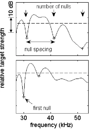
Figure 2-3: Example of automated structure analysis results. Plus signs indicate nulls and horizontal dashed lines indicate mean target strength of frequency band displayed. An example of the two criteria for a null are illustrated in the lower plot: (1) The dip near 42 kHz does not meet the criterion of 1 dB less than both adjacent peaks (2) The dip at 47 kHz does not meet the criterion of 3 dB less than the average of the two adjacent peaks.

2.4.2

Spectral classification

Acoustic scattering spectra of marine organisms are characterized by unique inter-ference patterns specific to target size, shape, material properties, and orientation

(Stanton et al., 1998b; Lavery et al., 2002; Reeder et al., 2004). In order to perform a quantitative, statistical analysis of the prey echoes compiled in this study, an algo-rithm was created to quantify the structure of the spectra. Once the echoes of interest were identified, the time series was filtered using a 20 to 70 kHz 4-pole Butterworth bandpass filter, and windowed using a 400 microsecond rectangular window. This result was then converted to a frequency spectrum using a Fourier transform.

The frequency band between 27 and 54 kHz was selected for analysis. This range falls within the -10 dB endpoints of the power spectrum of the transmitted signal and is limited to the range of frequencies where FM clicks have been shown to be nearly featureless as discussed in Sec. 2.2. Given the limited ENR of echoes selected for this study, three simple robust parameters were chosen to characterize the frequency response of the scatterers: (1) number of nulls, (2) location of first null, and (3) spacing of the first two nulls (Fig. 2-3). Nulls were identified by a greater than 3 dB difference between a local minimum and the average of two adjacent maxima. Nulls of less than 1 dB from either adjacent peak were discarded to minimize false detection of nulls. These limits were set so as to discriminate between nulls due to scattering phenomena and other sources of spectral structure such as variability in the source and ambient noise.

2.4.3

Target strength calculations

Estimated target strength of the scatterer was found using the active sonar equation (Urick, 1983).

T S = EL + 2T L − SL (2.1)

For these calculations only target strength, T S, and the received echo level at the transducer, EL, were allowed to vary with frequency, f , as explained below. T L and SL are one-way transmission loss and source level respectively. All values are calculated in terms of dB re 1 µP a. The echo level is determined from the raw

time-voltage signal, y(t) using the expression

EL(f ) = 20 log Y (f ) − S (2.2)

where Y (f ) is the discrete Fourier transform of y(t) and S is the sensitivity of the tag in dB re V /µP a.

Transmission loss, accounting for spherical spreading and absorption losses, was determined by the relation T L = 20 log r+αr, where r is one-way distance from trans-ducer to scatterer and α is absorption loss. The frequency dependence of absorption was neglected as the effect on transmission loss over the short target distances and range of frequencies considered here was small (< 0.5 dB). Thus, alpha was considered a constant: α ' 11 dB

km @ 40 kHz (Urick, 1983).

Source levels have not yet been measured for this species; therefore, all target strength values are presented in relative terms. A constant source level, i.e. constant at each frequency within the band, was chosen to represent the featureless portion of the whale’s transmitted signal. This notional source level, SLk, was adjusted for

variation in the apparent output of the transmitted click corresponding to each echo using the formula: SL = SLk + [AO − AO], where AO is the apparent output of a

specific click and AO is the mean apparent output of all regular clicks associated with echoes analyzed. As discussed in Sec. 2.3, it is believed that this provides a reasonable method for estimating fluctuations in the source level and, therefore, improves the precision of relative target strengths.

Target strength, T S, can be further defined as the logarithmic measure of the backscattered energy and is given by

T S = 10 log σbs (2.3)

where σbs is the differential backscattering cross section. Mean target strength of an

individual echo was found by averaging σbs(f ) over all frequency bins within the band

14

16

18

20

₃₀

40

50

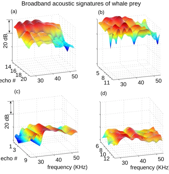
echo #

20 dB

5

8

11

₃₀

40

50

1

3

9

₃₀

40

50

frequency (KHz)

echo #

20 dB

6

8

10

12

30

40

50

frequency (KHz)

Broadband acoustic signatures of whale prey

Figure 2-4: Broadband acoustic signatures of four prey selected by the whale. Each plot is comprised of frequency spectra of a series of echoes that make up one echo train. Plots only include spectra from echoes within each train that met the criteria discusses in Sec. 2.4.1. Echoes represented are identified by a tick mark on the “echo #” axis. Figures (a) and (b) show examples of high target strength prey found at deep depths (below 700 m) in low echo density environments. Figures (c) and (d) show examples of lower target strength prey found in shallower water (above 700 m) in high echo density environments.

2.5

Results

2.5.1

Echoes selected for analysis

A total of 89 buzzes were observed during the three dives analyzed indicating possible predation events. Of these, 47 were preceded by unambiguous echo trains that are believed to correspond to scattering from prey. The remaining buzzes were associated with either irresolvable echo trains due to a cluttered environment or no echo trains with sufficient ENR. Additionally, in the echograms of dive #3, where a high percent-age of buzzes could not be correlated with echo trains, it is suspected that many echo trains existed but were obscured by reverberation from the bottom. The first echo of each train was discernable from background noise at varying TWT’s equivalent to a distance to the scatterer of between 5 and 15 m. In each case the echo train terminated shortly before the start of the buzz at a distance of 3 to 5 m.

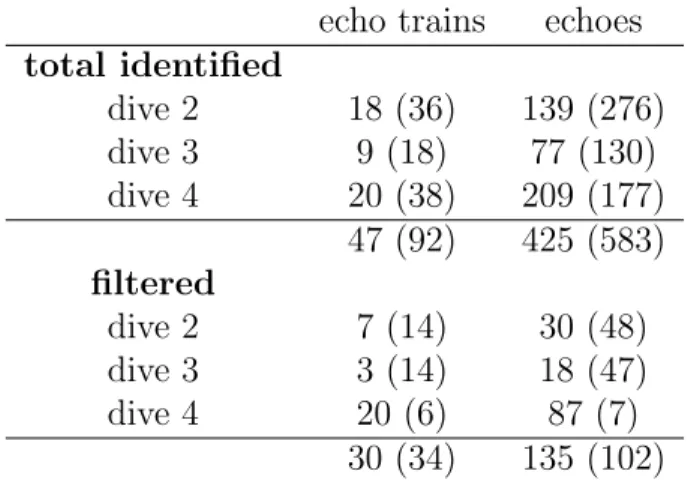
The 47 echo trains identified as prey selected by the whale contained a total of 426 discrete echoes. Of those 135 echoes from 30 different echo trains, met the criteria for sufficient ENR and for angle of arrival within ±4◦_{. In order to accumulate a sufficient}

number of non-selected echoes as a control, 92 echo trains from random scatterers, not selected as prey by the whale, were chosen. Of these 34 trains containing 102 echoes remained after following the same procedure. Distribution of the echoes over the three dives analyzed is shown in Table 2.1. Many more random, non-selected echo trains were required to obtain a similar sample size as they generally had fewer echoes in each train. This is likely due to the shorter length of time that these non-pursued scatterers remained within the whale’s acoustic beam.

2.5.2

Echo classification

Characterization of echo trains for comparison

A comparison was conducted between echo trains from scatterers selected by the whale and a non-selected control set based on spectral complexity and relative target strength. The primary focus of this study is to investigate whether or not the whales

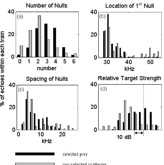
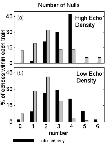
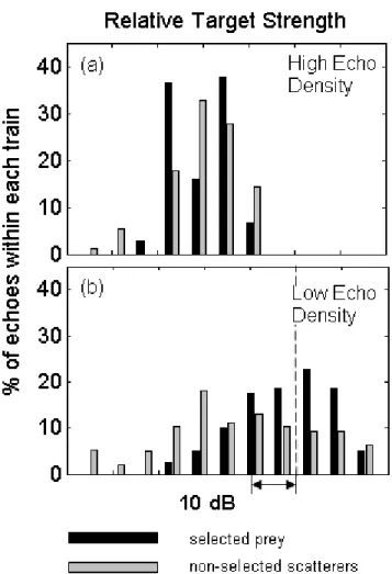
Figure 2-5: Normalized distribution of prey “selected” by the whale, and randomly chosen “non-selected” scatterers, i.e. not pursued by the whale as prey, (black and grey bars respectively) that contain a given characteristic: (a) number of nulls, (b) first null location, (c) spacing of first two nulls, and (d) relative target strength. Bins represent characteristics of a given echo within an echo train. Echoes are weighted by their fraction of the total number of echoes within a train. Distributions are normalized by the total number of echo trains (selected or non-selected). Vertical dashed line in target strength plot (d) represents absolute target strength value of -65 dB based on a source level of 200 dB.

Table 2.1: Distribution of echoes from selected and non-selected (in parenthesis) echo trains among three dives examined. Filtered echoes are limited to echo-to-noise ratio,

ENR, of 8 dB and angle of arrival, AOA of ±4◦_{. Echo trains used in averaged results}

had a minimum of 2 echoes per train.

echo trains echoes total identified dive 2 18 (36) 139 (276) dive 3 9 (18) 77 (130) dive 4 20 (38) 209 (177) 47 (92) 425 (583) filtered dive 2 7 (14) 30 (48) dive 3 3 (14) 18 (47) dive 4 20 (6) 87 (7) 30 (34) 135 (102)

are discriminating between echoes with different characteristics. Since the spectra of discrete echoes from a single marine organism can vary significantly with small changes in the scatterer’s orientation (Reeder et al., 2004), it is possible that distinct, but complementary information is obtained by the whale from multiple aspects of a single target. For these reasons the characteristics of individual echoes within each echo train, with no averaging, are considered in the statistical analysis performed on the data. Results presented here are shown as the number of echoes, as a percentage of the echo train in which they are contained, that exhibit a given spectral feature or target strength. The results are normalized by the total number of echo trains in the specific category, i.e. whale-selected group or non-whale-selected control group. It is believed that this method best reduces biases caused by the disproportionate length of some echo trains and also enables the classification of the echo trains according to one or more distinct features.

In addition to this method, two other statistical methods were used to analyze the echoes. One comparison was conducted on the echoes as a whole. In this method it was necessary to discard duplicate characteristics within an echo train to reduce the bias caused by echo trains of different lengths. The drawback of this method

was that, by removing redundant features within an echo train, key characteristics that may be used by the whale could be diluted through removal of an unrelated bias. Finally, an analysis was conducted by averaging the characteristics over each echo train. The effect of averaging is to smooth the frequency response patterns. In particular, sharp individual nulls in a discrete spectrum may become broad dips in an averaged frequency response. It is suspected that this approach may remove some subtle features of the echoes used by the whale in discriminating prey from other acoustic clutter. These concerns notwithstanding, good agreement was found in the primary results of all three methods. Only results of the first method, which present the data in the most raw form, are presented here.

Spectra

Results of the spectral analysis showed that significant structure exists, quantified by the number of nulls within the frequency band examined, in the frequency responses of many ensonified targets. As detailed in the data analysis section, it is believed that interference due to noise and beam pattern effects can be discounted as a major contributor to this structure. If noise were a significant contributing factor to the spectral structure, a trend towards a lower ENR for echoes containing more nulls would be expected as these echoes would be more susceptible to this interference. However, a comparison of number of nulls and ENR over all angles of arrival did not show such a trend. Instead the comparison showed only a 3 dB decrease in echo-to-noise ratio from 0 to 2 null targets and, most notably, a flat trend from 2 to 6 nulls. Furthermore, no correlation was found between number of nulls and angle of arrival,

θbeam. This supports the assumption that the constraint of a narrow range of arrival

angles has removed any distortion effects due to the angular offset within the whale’s sonar beam.

Figure 2-5a shows a comparison of the number of nulls in the frequency spectra of echo trains selected by the whale and non-whale-selected echo trains from all dives examined. One can see that there is a bias, in the echo trains from scatterers selected as prey, towards more highly structured returns (selected mean: 3.06, non-selected

mean: 2.12). A t-test showed that the difference was significant (t = 2.803, df = 63, p-value = 6.72 × 10−3_{). Notably, less than 2% of the selected echo trains were}

characterized by a featureless echo (i.e. an echo with no nulls), whereas nearly 10% of the non-selected echo trains were composed of such echoes. These results are contrary to that which would be expected if echo structure was primarily due to effects of the off-axis beam pattern. Non-selected targets are more slightly more likely to fall on the edge of the transmitted beam pattern, θbeam ≥ ±3deg, (non-selected: 24.5%,

selected: 20.0%), probably because they are not being actively pursued by the whale. However, a bias in structure content due to location in the beam, which would be expected if beam pattern effects were strong, is not seen.

A comparison of the different structure features between the selected and non-selected echo trains was less revealing. Figure 2-5 (b and c) compare the the whale-selected and non-whale whale-selected distributions of first null locations and spacings of the first two nulls, respectively. These results did not appear to have normal distributions and a Kolmogorov-Smirnov test showed no significant difference in the distributions (null location: k = 0.290, p-value = 0.131, null spacing: k = 0.232, p-value = 0.381). The spacing of the nulls did appear to have a bi-modal (selected) and multi-modal (non-selected) distribution.

Target strengths

Echo trains selected by the whale are composed of echoes that have a target strength distribution that is shifted approximately 18 dB higher than non-selected echo trains (Fig. 2-5d). A Kolmogorov-Smirnov test rejected the null hypothesis that the two samples were from the same distribution (k = 0.400, p-value = 7.22 × 10−3_{). It is also}

observed that echo trains from selected prey showed wide echo to echo variation in target strength with 60% containing echoes that varied by 9 dB while 17% contained echoes varying by at least 15 dB. Non-selected echo trains had less variability with only 26% of echo trains having a 10 dB variation and 15% varying by at least 15 dB. This difference in variability between selected and non-selected echo trains may be a factor of the fewer number of echoes, on average, in the non-selected echo trains.

150

200

250

300

350

400

500

600

700

800

900

1000

1100

1200

1300

time (min)

depth (m)

Prey Distribution

HI PREY DENSITY

LO PREY DENSTIY

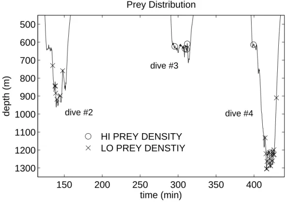
Figure 2-6: Depth distribution of prey categorized by echo density. Depth is truncated above 450 m as no predation events were found at shallower depths.

2.5.3

Comparison of echo characteristics between two groups

of prey

Echo characteristics of two groups of prey, which were separated by depth and differed in aggregation density, are compared. It is suspected that two distinct prey categories can be defined by comparing discrete backscattering by prey in a deep, low echo density aggregation with prey in a shallow, high echo density aggregation. Echo density, in regions where the whale hunted, varied widely during the three dives (Fig. 2-2). Prey aggregations on dive #2 and #4 were characterized by low density while dive #3 was nearly exclusively high echo density. The two suspected prey categories were separated spatially in the water column with the high density group in water shallower than 700m and lower density group found at greater depths (Fig. 2-6).

In the shallow, high echo density aggregation, differences in the number of nulls be-tween selected and non-selected targets is shown to not be significant by a

Kolmogorov-Figure 2-7: Spectral content in frequency responses of prey selected by the whale and non-whale-selected scatterers (black and grey bars respectively) in: (a) shallow, high echo density aggregations, and (b) deep, low echo density aggregations. Weighting and normalization are identical to Fig. 2-5.

Smirnov test (k = 0.447, p-value = 0.318) and may have suffered from small sample size (Fig. 2-7a). However, as in the combined results of all prey targets, discussed in Sec. 2.5.2, the targets selected by the whale in the low echo density aggregation were characterized by more highly structured echoes than the control group of non-selected targets (Fig. 2-7). A t-test showed that the difference in means (selected: 2.96 nulls, non-selected: 1.85 nulls) was significant (t = 3.186, df = 40, p-value = 2.80 × 10−3₎

size available.

The target strength distribution provided further information about these two scattering groups. The target strength distribution between selected and non-selected echo trains in both echo density environments were heavily overlapping (Fig. 2-8). No significant difference was found using Kolmogorov-Smirnov tests in either case (high echo density: k = 0.178, p-value = 0.999; low echo density: k = 0.340, p-value = 0.140). However, when scatterers from the two environments are compared it can be seen that there is at least a 15 dB shift in the target strength distributions.

2.5.4

Comparison between echo characteristics and

scatter-ing predictions/observations

Target strength variability

In Sec. 2.5.3. a significant difference in the target strength distribution is shown between a shallow, high echo density aggregation and a deep, low echo density ag-gregation. Using a simple, straight finite cylinder model for weakly scattering marine organisms of length L, it is seen that in the geometric scattering region target strength varies as 10 · log(L2_{), (Stanton et al., 1993, 1994). This first order approximation can}

be used to estimate a ratio of the prey lengths from the difference in target strengths. For broadside scattering from two organisms of roughly the same aspect ratio and material composition, a 15 dB difference in target strengths correlates to a length factor of approximately 5.5. The fact that this whale dives to significantly greater depths, i.e. an additional 500 to 600 m, to pursue a type of prey found in less dense aggregations is counterintuitive. However, the possibility that the prey found at depth are significantly larger may be one explanation for this behavior.

Effects of orientation

In another study an acoustic scattering model for squid has been developed. This is based on a weak-scattering theory using high resolution spiral computerized tomog-raphy (SCT) scans. Predictions of target strengths from small squid have been made

Figure 2-8: Reduced target strength distribution of prey selected by the whale and non-whale-selected scatterers (black and grey bars respectively) in: (a) shallow, high echo density aggregations, and (b) deep, low echo density aggregations. Vertical dashed line represents absolute target strength value of -65 dB based on source level of 200 dB. Weighting and normalization are identical to Fig. 2-5.

over a range of angles and orientation. In the analysis of whale-prey echoes, signif-icant ping-to-ping variability in both structure content and target strength if found to exist within some echo trains selected by the whale (Fig. 2-4a and b). Because the transmitted signal of the whale has been constrained to near on-axis signals, vari-ations presumably relate to the orientation of the scatterer relative to the incident sound wave. Modeling predictions for squid show a similar variability. The interfer-ence pattern and magnitude of the frequency response are highly affected by changes

in the aspect of the scatterer with respect to the incident sound wave. Measured broadband scattering from fish have shown similar results with changes as small as 5 degrees dramatically changing the backscattered frequency response (Reeder et al., 2004).

2.6

Discussion

The characteristics of broadband echolocation signals have been studied through data obtained, in situ, by a recording device mounted on a foraging Blainville’s beaked whale. By setting stringent criteria on the echoes analyzed and, in part, due to the opportunely smooth spectrum of the M. densirostris’ emitted signal, the spec-tral characteristics of the prey’s frequency responses can be analyzed over a limited frequency range and relative target strengths can be estimated.

Significant structure, resembling the type of interference patterns observed from marine organisms in modeling and laboratory experiments, exist in the frequency spectra of prey echoes measured in this study. It has been concluded that structure contained within the frequency responses of scatterers is consistent with, and most likely due to, interference from multiple wave interactions incurred by the morphology, material properties, and orientation of the scatterer.

A combination of whale depth and echo density was combined with the scattering results to show that it is likely that the whale preyed upon at least two different types of organism with different target strength distributions. This whale hunted a low target strength population found in high density aggregations between depths of 600 and 650 m. Higher target strength prey were found at various depths below 700 meters in low echo density environments. In neither case was a significant differ-ence found in the target strength distributions between prey selected by the whale and a control group of non-whale-selected scatterers. This suggests that the target strength of a scatterer is not the whale’s sole means of discriminating between prey and non-prey targets. It is significant that, for at least the low echo density case, this animal appeared to favor targets that display a higher degree of structure within

their frequency responses. It is not possible to confirm, however, that this whale is using specific structural features, such as null location or spacing, in recognizing or classifying specific prey items.

Finally, an explanation has been proposed as to why this large marine predator chooses to dive to significantly deeper depths to hunt less dense populations of prey. Scattering theory for weakly scattering, non-swimbladder bearing marine organisms suggests that the higher target strength organisms found at depth could be 5 to 6 times the size of prey hunted in shallower water, thus giving the animal an incentive to expend the energy required to dive to greater depths.

Chapter 3

Acoustic scattering by weakly

scattering shelled objects:

Application to Squid

1

3.1

Introduction

A model has been developed, based on the distorted wave Born approximation (DWBA), to predict acoustic scattering from arbitrarily shaped, arbitrarily inhomogeneous, weakly scattering volumes. Although the DWBA formulation, in principle, can ac-count for 3-D material property inhomogeneities, significant obstacles are enac-countered when applying this model to a randomly inhomogeneous object. In the Born approx-imation the amplitude and phase of the incident wave are only dependent on the position of the wave front with respect to some arbitrary origin and the material properties of the surrounding medium. This is due to the general assumption that the incident wave is unmodified by the weakly scattering body. In contrast, the DWBA is a modification to the Born approximation in which the wavenumber in-side the scattering volume is determined by the material properties within the body (Stanton et al., 1993). Thus, the phase of the wavefront, at any point in the volume,

1_{This chapter is based on an article to be submitted to the Journal of the Acoustical Society of}

is dependent both on the distance traveled by the incident wave and any sound speed variations encountered along the path traveled.

As discussed in Ch. 1, the DWBA has been applied to homogeneous scattering volumes and volumes with material properties that vary only in one dimension. In these cases the DWBA formulation can be applied directly, either to the body as a whole or, in the axially varying case, to each cross section separately assuming normal incidence of the sound wave. The primary advance made in this study is correctly accounting for the phase of the incident wave as it travels through an inhomogeneous medium. The numerical incorporation of this method uses a ray trace component to track the phase at every position within the scattering volume. A two part algorithm calculates phase and amplitude for every discretization before integrating over the entire volume. Application of this DWBA ray-tracing model to squid is discussed in detail.

Although relatively little work has been published on acoustic scattering models of squid there is interest in this research from two areas. The first is commercial fish-eries. As a fast growing but short-lived species, squid are particularly vulnerable to overfishing (Goss et al., 2001). Acoustic stock assessments can be use to complement more traditional techniques such as trawl surveys and fishery catch analyses by rapidly surveying large volumes of water and providing real time population assessments (re-view by Starr and Thorne (1998)). Understanding the factors that influence sound scattering from squid is clearly essential for reliable surveys of this type. Secondly, there is increasing interest in the predator-prey relationship between echolocating ma-rine mammals and squid. Beaked whales, for instance, hunt squid using broadband, ultrasonic sonar (Johnson et al., 2004; Madsen et al., 2005). Scattering models that help define the dominant scattering mechanisms of squid may elucidate factors that are exploited by the whales in discriminating between prey and non-prey.

The DWBA ray-tracing model is applied to long-finned squid, (Loligo pealeii). Density and sound speed measurements of squid suggest that these invertebrates are well suited to modeling as weak scatterers (Mukai et al., 2000; Kang et al., 2004; Iida

spher-oid model (LPSM) and the DWBA formulation, also using prolate spherspher-oid geometry (Arnaya and Sano, 1990b; Mukai et al., 2000). These models assume homogeneous material properties within the scattering volume. In this study high-resolution spiral computerized tomography (SCT) scans have been used to obtain 3-D morphology of squid. Unlike previous DWBA models of squid, the DWBA ray-tracing model incorporates the complex mantle structure by differentiating between seawater filled cavities and the squid’s body. Material property variation due to internal organs, however, is not included in this study. Predictions are compared with published results of both anesthetized, tethered squid and live, freely swimming squid.

Application of the DWBA ray-tracing model is presented in two parts. First, to validate the model, it is applied to simple geometric shapes of both homogeneous and inhomogeneous material composition. Target strength predictions are compared with solutions to modal-series-based formulations, and existing DWBA scattering models defined in Sec. 3.2. Acoustic scattering predictions, given in Sec. 3.4.1, are calculated for simple geometric objects with variations in material properties, shell thickness, and orientation. Second, the DWBA ray-tracing model is applied to squid of the species L. pealeii. In order to compare scattering predictions with actual scattering measurements, the model is extended to a second species of squid T. pacificus by digitally scaling the 3-D morphological measurements of squid used in the model. Comparisons of predicted target strengths with published target strength data for this species are shown in Sec. 3.4.2.

3.2

Theory

3.2.1

Basic definitions

Acoustic scattering from an object in the far field is described in terms of the ampli-tude of the incident sound wave, P0, and the scattering amplitude, f ,

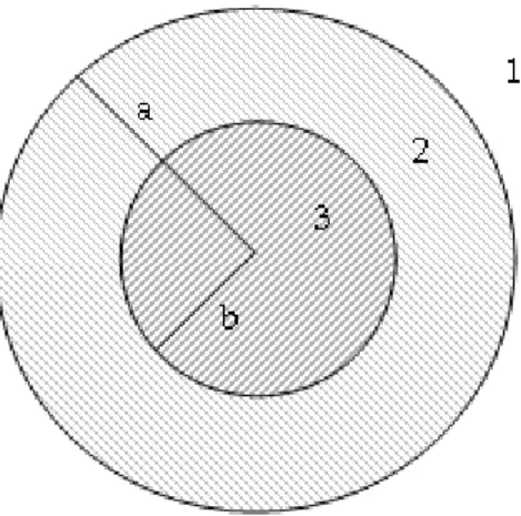
Figure 3-1: Bisection of spherical shell or cross section of cylindrical shell. Indices 1-3 correspond to fluids of different material properties (i.e. sound speed, ci, and density,

ρi, i = 1, 2, 3). The radii a and b are the outer and inner shell radii respectively such

that (a − b)/a corresponds to fractional shell thickness, τ .

Pscat= P0 eik1r

r f (3.1)

where, r is the distance from the object to the receiver. The acoustic wavenumber of the surrounding medium, k1, is defined as 2π/λ, where λ is the acoustic wavelength.

Target strength is the logarithmic measure of the backscattered energy, expressed in decibels, dB, relative to m2_.

T S = 10 log σbs (3.2)

where σbs = |fbs|2 is the differential backscattering cross section and fbs, or

backscat-tering amplitude, is f evaluated in the backscattered direction. Mean target strength is found by averaging σbs prior to logarithmic conversion as hT Si = 10 loghσbsi.

In order to compare scattering from objects that are similar in proportion but of different overall size, reduced target strength, RT S, is often used. For a sphere or