HAL Id: insu-01408629
https://hal-insu.archives-ouvertes.fr/insu-01408629
Submitted on 5 Dec 2016
HAL is a multi-disciplinary open access
archive for the deposit and dissemination of
sci-entific research documents, whether they are
pub-lished or not. The documents may come from
teaching and research institutions in France or
abroad, or from public or private research centers.
L’archive ouverte pluridisciplinaire HAL, est
destinée au dépôt et à la diffusion de documents
scientifiques de niveau recherche, publiés ou non,
émanant des établissements d’enseignement et de
recherche français ou étrangers, des laboratoires
publics ou privés.
Swarm’s absolutemagnetometer experimental
vectormode, an innovative capability for space
magnetometry
Gauthier Hulot, Pierre Vigneron, Jean-Michel Léger, Isabelle Fratter, Nils
Olsen, Thomas Jager, François Bertrand, Laura Brocco, Olivier Sirol, Xavier
Lalanne, et al.
To cite this version:
Gauthier Hulot, Pierre Vigneron, Jean-Michel Léger, Isabelle Fratter, Nils Olsen, et al.. Swarm’s
absolutemagnetometer experimental vectormode, an innovative capability for space magnetometry.
Geophysical Research Letters, American Geophysical Union, 2015, �10.1002/2014GL062700�.
�insu-01408629�
RESEARCH LETTER
10.1002/2014GL062700Special Section:
ESA’s Swarm Mission, One Year in Space
Key Points:
• First geomagnetic field model derived from absolute vector data
• Monitoring the magnetic field from space with a simplified payload is possible
Correspondence to:
G. Hulot, [email protected]
Citation:
Hulot, G., et al. (2015), Swarm’s abso-lute magnetometer experimental vector mode, an innovative capa-bility for space magnetometry,
Geophys. Res. Lett., 42, 1352–1359,
doi:10.1002/2014GL062700.
Received 6 DEC 2014 Accepted 29 JAN 2015
Accepted article online 2 FEB 2015 Published online 4 MAR 2015
Swarm’s absolute magnetometer experimental vector mode,
an innovative capability for space magnetometry
Gauthier Hulot1, Pierre Vigneron1, Jean-Michel Léger2, Isabelle Fratter3, Nils Olsen4, Thomas Jager2, François Bertrand2, Laura Brocco1, Olivier Sirol1, Xavier Lalanne1, Axel Boness2, and Viviane Cattin2
1Equipe de Géomagnétisme, Institut de Physique du Globe de Paris, Sorbonne Paris Cité, Université Paris Diderot, UMR
7154 CNRS/INSU, Paris, France,2CEA, Léti, Grenoble, France,3Centre National d’Etudes Spatiales, Toulouse, France,
4DTU Space, National Space Institute, Technical University of Denmark, Kongens Lyngby, Denmark
Abstract
European Space Agency’s Swarm satellites carry a new generation of4He absolutemagnetometers (ASM), designed by CEA-Léti and developed in partnership with Centre National d’Études Spatiales. These instruments are the first ever spaceborne magnetometers to use a common sensor to simultaneously deliver 1 Hz independent absolute scalar and vector readings of the magnetic field. Since launch, these ASMs provided very high-accuracy scalar field data, as nominally required for the mission, together with experimental vector field data. Here we compare geomagnetic field models built from such ASM-only data with models built from the mission’s nominal 1 Hz data, combining ASM scalar data with independent fluxgate magnetometer vector data. The high level of agreement between these models demonstrates the potential of the ASM’s vector mode for data quality control and as a stand-alone magnetometer and illustrates the way the evolution of key field features can easily be monitored from space with such absolute vector magnetometers.
1. Introduction
Swarm, the fifth Earth Explorer Mission in the Living Planet Programme of the European Space Agency (ESA)
was launched on 22 November 2013. It consists of a constellation of three identical satellites and aims at studying all aspects of the Earth’s magnetic field [Friis-Christensen et al., 2006]. Two satellites (Alpha and Charlie) fly almost side by side on low-altitude polar orbits (inclination of 87.4◦, with longitude separation of 1.4◦, altitude of about 470 km above a mean radius of a = 6371.2 km in November 2014). The third satellite (Bravo) is on a similar, but slightly more polar and higher orbit since April 2014 (88◦inclination and 520 km altitude in November 2014) to allow for a progressive local time separation with respect to Alpha and Charlie (about an hour in November 2014). Each satellite carries a magnetometer payload consisting of three instruments, all mounted on a boom to minimize mutual interferences and perturbations caused by the satellite itself. Two are mounted close to each other on a common rigid optical bench: the Vector Fluxgate Magnetometer (VFM), which measures the direction and strength of the magnetic field, and the three-head Star TRacker (STR), which provides the attitude information needed to transform the vector readings to a known terrestrial coordinate frame. The third instrument, the Absolute Scalar Magnetometer (ASM), is located 2 m farther down the satellite’s boom and provides absolute measurements of the magnetic field intensity. The payload also includes a GPS and instruments to measure plasma and electric field parameters as well as gravitational acceleration. More information about the mission can be found in (R. Floberghagen et al., The Swarm mission—An overview one year after launch, Earth Planets and Space, in review, 2015). The nominal role of the ASMs is to provide very accurate 1 Hz absolute scalar readings of the magnetic field for both science and VFM in-flight calibration purposes. In addition, and thanks to an innovative design, these instruments can also use the same sensor to deliver 1 Hz independent vector readings of the magnetic field [Gravrand et al., 2001; Léger et al., 2009]. Following an agreement between ESA and Centre National d’Études Spatiales, who funded the development of the ASM instruments and provided them as customer furnished instruments, this possibility has been used on an experimental basis since the beginning of the mission. Analysis of the corresponding experimental vector data (hereafter referred to as 1 Hz ASM_V data) during the calibration and validation activities have led to very encouraging results (I. Fratter et al., Swarm absolute scalar magnetometers first in-orbit results, Acta Astronautica, in review, 2015), leading to the
Geophysical Research Letters
10.1002/2014GL062700
possibility of building geomagnetic field models entirely based on these experimental ASM_V data, as if no VFM data were available. The present letter reports on such a model, which we compare to analogous models built in exactly the same way and using the same data distribution but relying on nominal Level 1b data (hence VFM, rather than ASM_V data). This comparison not only reveals the capability of the ASM instruments to provide science class data as a stand alone absolute vector magnetometer but also highlights the value of having such an ASM vector mode available on board the Swarm mission for data quality control and possible improvement.2. ASM Principle and Vector Mode
The ASM instrument is first and foremost an absolute scalar magnetometer, which measures the field strength by detecting and quantifying the Zeeman splitting between the three sublevels of the 23S
1
metastable state of4He. The energy separation between these sublevels is directly proportional to the field
strength and is measured by magnetic resonance using a radio frequency signal. The frequency f of this signal is such that B0= f ∕𝛾 when resonance occurs, where 𝛾 is the known and constant4He gyromagnetic
ratio for the 23S
1state, and B0the field intensity to be measured. Using a laser selective pumping process
allows the resonance signal to be enhanced, increasing the sensitivity of the instrument by several orders of magnitude [Guttin et al., 1994]. Specific polarization conditions with respect to the direction of the ambient field must, however, be maintained. This is achieved by using a piezoelectric motor to rotate parts of the instrument. A key advantage of this instrument is that its intrinsic bandwidth allows scalar data to be acquired at 250 Hz, corresponding to 100 Hz bandwidth measurements. This possibility can be taken advantage of in two ways. First, to assess the noise level of the instrument, and second, to use three orthogonal sets of coils fitted on the instrument, each producing magnetic modulations with well-controlled amplitudes (50 nT) and frequencies (adequately chosen within the 1–100 Hz frequency range) that add up to the natural field B0(t), to also infer the components of this field along the three (perpendicular) coil axis, using real-time deconvolution of the resulting scalar field|B0(t) +∑3i=1bicos(𝜔it)|
[Gravrand et al., 2001; Léger et al., 2009].
Contrary to the scalar field measurement B0(t) of|B0(t)|, the 1 Hz field components recovered in this way
are not absolute and need to be calibrated. This calibration process is analogous to the one used for fluxgate magnetometers [Merayo et al., 2000]. It allows for slight nonorthogonality and possible thermal expansion of the coils, the corresponding calibration parameters being recovered by requesting the reconstructed field modulus to match the scalar estimate B0(t), using a large enough set of data as input [see Gravrand et al.,
2001]. The instrument’s setup, however, has several key advantages. Because the same sensor is being used to simultaneously recover scalar and vector field estimates, filtering and synchronization errors are suppressed. Likewise, possible external perturbations will have no influence on the calibration process, and biases between vector and scalar readings can be ignored altogether. These advantages come at a cost, though: by design, the resolution in the vector components will be degraded by a factor ∼ 103(at B
0= 25𝜇T)
compared to the scalar measurements. But the resolution and accuracy of the scalar measurements are extremely good (1.0–1.4 pT/√Hz depending on the instruments and 65 pT at most, respectively, over [DC-100 Hz] as inferred from the analysis of 250 Hz data). Monitoring of the scalar residuals (difference between the scalar estimate and the modulus of the vector estimate) after calibration (done on a daily basis, using data over the day of interest, the previous day, and the day after) revealed a raw noise level on the order of𝜎 =2.7 nT (root-mean-square (RMS) value of the scalar residual, with no bias) for the 1 Hz ASM_V data on the Alpha and Bravo satellites, that could be reduced to𝜎 ≤ 2 nT by avoiding data close to piezoelectric motor activations. A somewhat higher noise was found in the ASM_V vector data of the third, Charlie, satellite (for more details, see I. Fratter et al., in review, 2015).
3. Data Selection
Only the better Alpha and Bravo 1 Hz ASM_V data were considered, between 29 November 2013 and 6 November 2014. This was not a critical limitation since Charlie and Alpha were orbiting very close to each other, compared to the length scales of the models to be built, and no use was made of gradient data (for a demonstration of the usefulness of gradient data using Charlie, see Olsen et al. [2015] this was not a critical limitation. Some data were removed manually, based on early inspection of the ASM_V data: 27 January to 6 February 2014 for Alpha, and on 5 December 2013 between 09:36 and 12:00, and
between 8 and 17 December 2013 for Bravo. Only data from dark regions were used (Sun at least 10◦ below the horizon), to minimize unmodeled ionospheric signals. The strength of the magnetospheric ring current, estimated using the ring current (RC) index (see Olsen et al. [2014] and section 4), was required to change by at most 2 nT/h, while geomagnetic activity was required to be such that the geomagnetic index Kp≤ 2+.
At quasi-dipole (QD) latitudes [e.g., Richmond, 1995] poleward of ±55◦, only scalar ASM data were considered (to avoid unmodeled field-aligned current signals) and it was additionally required that the weighted average over the preceding hour of the merging electric field at the magnetopause [e.g., Kan
and Lee, 1979] was not too large (Em< 0.8 mV/m, as defined in Olsen et al. [2014]). For other latitudes, only ASM_V vector data were used, with the extra requirement that the scalar residual was less than 0.3 nT and the ASM piezoelectric motor had not been activated within the previous 3 s. In both cases, the resulting data sets were decimated (by a factor of 4 for vector data and 34 for scalar data, amounting to an average time separation between successive data of roughly 21 and 33 s, for vector and scalar data, respectively) to avoid oversampling along satellite tracks, while still providing a large enough data set for the present purpose. Finally, additional mild selection criteria were added to ensure the availability, for each selected ASM_V datum, of a meaningful equivalent official L1b vector datum at exactly the same time on the same satellite, with vector field components within 500 nT (and scalar field within 100 nT) of predictions from the CHAOS-4 model of Olsen et al. [2014] (up to degree and order 20). This made it possible to match the resulting ASM-only data set by two additional data sets, with exactly the same amount of data at exactly the same times and locations, which we used for model comparison purposes: a L1b data set, which used an official L1b VFM vector datum in the VFM instrument frame (release 0302 when available, otherwise release 0301) in place of each ASM_V vector datum; and a normalized L1b data set, identical to the L1b data set, except for the fact that each vector datum was further normalized to have a modulus equal to the synchronous ASM scalar datum. Note that for all three data sets, vector components were provided in the corresponding instrument’s frame (ASM_V frame for the ASM-only data set, VFM frame for the L1b and normalized L1b data sets). Each data set amounted to 3 × 145, 487 = 436, 461 vector and 31,515 scalar data from the Alpha satellite, and 3 × 162, 491 = 487, 473 vector and 33,338 scalar data from the Bravo satellite, amounting to a total of 988,787 data.
4. Model Parameterization and Estimation
Model parameterization was similar to that used for CHAOS-4 in Olsen et al. [2014], though simplified, and we refer the reader to this publication for detailed formulas and explanations. The field was assumed to be potential and harmonic with both internal and external sources.
Internal sources, which account for both the core and the lithospheric fields, were represented by a spherical harmonic expansion up to degree and order 45 (at reference radius a = 6371.2 km). Time changes through the period considered were taken into account via a constant secular variation up to degree and order 13. The parameters describing the internal part of the field thus consisted of 45 × 47 = 2115 static Gauss coefficients, and 13 × 15 = 195 secular variation Gauss coefficients.
External sources were described in a somewhat more sophisticated way but exactly following Olsen et al. [2014, equations (4) and (5)]. Two contributions were modeled. One corresponds to remote magnetospheric sources and is best described as a zonal external field of degree 2 in geocentric solar magnetospheric (GSM) coordinates, involving only two Gauss coefficients. The other corresponds to the near magnetospheric ring current and is best described in solar magnetic coordinates, up to degree and order 2. But this contribution is time varying and further induces an internal field. Its fast-varying part is described by a so-called ring current (RC) index, which is computed independently from observatory data, prior to the model computation (in the way described in Olsen et al. [2014]). This RC index is not enough, however, to properly model the ring current at satellite altitude, and three static regression factors plus a number of RC baseline corrections were coestimated during the model calculation. Referring to the notations of Olsen et al. [2014, equations (4) and (5)], the parameters we used for the external field thus were (101 in total) as follows: q01,GSM, q02,GSMfor the remote magnetospheric sources (two coefficients); qm
2, sm2 for the static degree 2 component of the ring
current (five coefficients);̂q0 1,̂q
1 1,̂s
1
1for the regression factors (three coefficients); Δq 0
1solved in bins of 5 days,
and Δq1 1, Δs
1
Geophysical Research Letters
10.1002/2014GL062700
Table 1. NumberNof Data Points, Mean, and RMS Misfit (in nT, Computed Using the Final Huber Weights) of Scalar at Polar (Poleward of±55◦) QD Latitudes (Fpolar), and of Field Aligned (Fnon-polar) andBr, B𝜃, B𝜙Vector Components at Nonpolar (Equatorward of
±55◦) QD Latitudes for Each of the ASM_V, VFM, and VFM_N Models
ASM_V VFM VFM_N N Mean RMS Mean RMS Mean RMS Alpha Fpolar 31,515 −0.25 3.71 −0.11 3.70 −0.10 3.69 Fnonpolar 145,487 0.10 2.53 −0.06 2.49 0.08 2.49 Br 145,487 0.00 2.46 0.01 1.81 0.02 1.85 B𝜃 145,487 −0.06 3.58 0.12 3.18 0.04 3.19 B𝜙 145,487 −0.11 2.92 −0.08 2.55 −0.09 2.54 Bravo Fpolar 33,338 −0.04 3.67 0.12 3.67 0.13 3.66 Fnonpolar 162,491 0.03 2.38 0.15 2.33 0.01 2.34 Br 162,491 0.04 2.39 0.04 1.71 0.04 1.78 B𝜃 162,491 0.03 3.43 −0.04 3.08 0.06 3.08 B𝜙 162,491 −0.11 2.82 −0.10 2.50 −0.10 2.49
Finally, we also solved for the Euler angles describing the rotation between the magnetometer (ASM or VFM) and STR frames. This was done by bins of 10 days, which implied solving for an additional 3 × 34 parameters per satellite, hence, 204 in total.
The total number of parameters to be estimated thus amounted to 2115 (static Gauss coefficients) + 195 (secular variation Gauss coefficients) + 101 (external field coefficients) + 204 (Euler angles) = 2615 parameters for each model. These model parameters were estimated from the 988,787 data, using an Iteratively Reweighted Least Squares algorithm with Huber weights. No regularization was applied and the cost function to minimize was simply eTC−1e, where e = d
obs− dmodis the difference between the vector
of observations dobsand the vector of model predictions dmod, and C is the data covariance matrix. A
geographical weight was introduced, proportional to sin(𝜃) (where 𝜃 is the geographic colatitude), to balance the geographical sampling of data. In all computations, anisotropic magnetic errors due to attitude uncertainty were taken into account assuming an isotropic attitude error of 10 arcsecs (recall, indeed, that even isotropic attitude error produces anisotropic magnetic errors, see Holme and Bloxham [1996], the formalism of which we rely on). A priori data error variances were otherwise set to 2.2 nT for both scalar and vector data. These numbers were chosen based on the expected combined effect of instrument noise and contributions from nonmodeled sources and are indeed reasonably consistent with the a posteriori data misfits (see Table 1). The (static) starting model did not influence the final model, and convergence was such that changes in the final misfits did not exceed 0.01 nT between the two last iterations.
5. ASM_V Versus L1b Model Comparisons
Three models were computed. An ASM_V model using the ASM_V data set (and thus entirely based on ASM data), a VFM model, using the nominal L1b data set, and a VFM_N model, using the normalized L1b data set. Note that whereas the ASM_V model truly ignores all VFM data, both the VFM and VFM_N models still rely on the ASM scalar data as provided in the L1b data. Table 1 shows the residual statistics for these three models, and Figure 1 shows the Lowes-Mauersberger spectra [Mauersberger, 1956; Lowes, 1966] of the field (at central epoch 22/4/2014, Figure 1a) and of the secular variation (Figure 1b) predicted by each model, together with all spectra of the two by two differences among models.
Comparing models ASM_V and VFM is what we are ultimately interested in, as it will reveal the impact of using the ASM_V data in place of the nominal VFM L1b data, i.e., the impact of the disagreement between the vector field information provided by the ASM and VFM instruments. But the impact of the disagreement between the instruments can also be investigated separately for the directional and norm disagreement by comparing models ASM_V and VFM_N, on the one hand, and models VFM and VFM_N, on the other hand. Recall, indeed, that models ASM_V and VFM_N use data sets that differ almost only because of directional disagreement (norms of the ASM_V vector data match the ASM scalar data to within 0.3 nT by selection and the VFM_N vector data are normalized to the ASM scalar data by construction, section 3) while models VFM and VFM_N use data sets that only differ because of norm disagreement.
Figure 1. (a) Lowes-Mauersberger spectra of the ASM_V (solid red), VFM (solid green), and VFM_N (solid blue) models for the field of internal origin at the
central epoch (22/4/2014), together with the spectra of differences among these models (ASM_V - VFM, dashed red; ASM_V - VFM_N, dashed green; VFM - VFM_N, dashed blue), all at ground surface; (b) Same but for the secular variation spectra.
Comparing the spectra of the ASM_V versus VFM (Figure 1, red dashed), ASM_V versus VFM_N (green dashed), and VFM versus VFM_N (blue dashed) differences reveals that directional disagreement has the greatest impact. Indeed, norm disagreement has an impact more than 1 order of magnitude smaller in spectral terms than the overall disagreement between the ASM_V and VFM vector data (except for the first two degrees of the secular variation, which happen to be more sensitive to errors in norm disagreements). This is further confirmed by looking at the residual statistics, which are much more similar for the VFM and VFM_N models than for the ASM_V and VFM (or VFM_N) models (Table 1).
In fact, Table 1 shows that the ASM_V model residual misfits differ significantly from those of the VFM and VFM_N models only when considering the vector components Br, B𝜃, and B𝜙. But even these differences are relatively modest. Roughly assuming the corresponding RMS misfit increases to be due to some independent source of vector field noise, this additional noise level would be on the order of 1.5 nT RMS. It would reflect the combined impact of the larger noise level of the ASM_V vector data compared to the VFM vector data and of unavoidable boom distortions between the ASM and the optical bench on which the VFM and the STR are mounted. Indeed, these 1.5 nT RMS are compatible with the total noise level in the ASM_V data (on the order of 2 nT RMS or less for the data selected, recall section 2). Even more importantly, they also are fully consistent with the order of magnitude of the boom deformation (with an average on the order of 10 arcsec, leading to a typical error of up to 2 nT in a 40.000 nT field) which we could indirectly infer between the ASM_V and the VFM instruments using the observed changes in the Euler angles (coes-timated every 10 days with the models, recall section 4). It thus is the limit of this mechanical link, probably more than the intrinsic noise level of the ASM_V data, that limits the overall quality of the ASM_V model. Figure 2 shows maps of the lithospheric and core fields as predicted by the ASM_V model (Figures 2a and 2e), maps of the way these differ from those predicted by the VFM and VFM_N models (Figures 2b, 2f, 2c, and 2g), as well as maps of the way these two VFM and VFM_N models differ (Figures 2d and 2h). Differences in the lithospheric parts of the ASM_V and VFM (or VFM_N) models (Figures 2b and 2c) are dominated by the smallest scales. They do not reveal any trivial pattern, except for a clear enhancement of errors close to the ±55◦QD latitudes, which the comparison of the VFM and VFM_N models (Figure 2d) reveals even better. This pattern is a consequence of the modeling choice of only selecting ASM scalar data poleward of ±55◦QD latitudes, thus producing an edge effect, enhanced when considering models with norm disagreement (i.e., when comparing the ASM_V or VFM_N models to the VFM model). Differences found in the ASM_V and VFM (or VFM_N) core fields are of a different nature. They tend to concentrate in zonal terms, and their pattern at satellite altitude (Figures 2f and 2g) clearly points at the cause of these differences being in orbital systematic ASM_V/VFM vector data disagreements on the order of a few nT. Systematic disagreements with similar order of magnitude have been identified between the norm of the L1b VFM vector data and the ASM scalar data, testifying for the occurrence of a “VFM-ASM disturbance field” presently under investigation (cf. R. Floberghagen et al., in review, 2015). We note, however, that the impact of this disturbance field would be less related to the error it introduces in the norm of the L1b VFM vector data (as testified by the little difference found between the VFM and VFM_N models, Figure 2h) than to the directional error it also potentially introduces. It thus is the combined effect of this disturbance field
Geophysical Research Letters
10.1002/2014GL062700
Figure 2. (left) Lithospheric and (right) core field model comparisons:Brforn= 15–45 at ground surface from (a) model ASM_V and from (b) ASM_V minus VFM,
(c) ASM_V minus VFM_N, and (d) VFM minus VFM_N model differences;Brforn= 1–13, central epoch 22/4/2014 from (e) model ASM_V at the core surface and
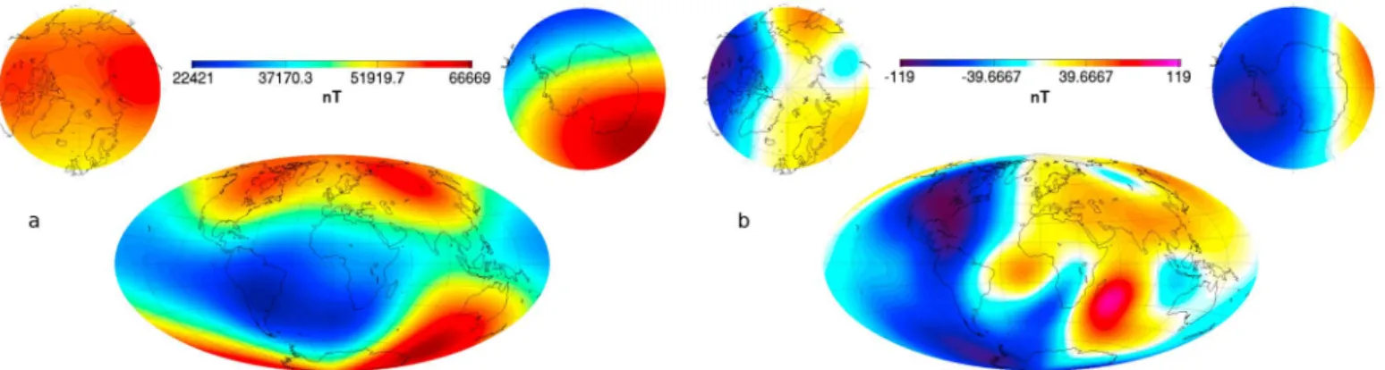
Figure 3. (a) Total field intensity at the Earth’s surface, as described by the ASM_V model for central epoch (22/4/2014); (b) Total field intensity change at the
Earth’s surface between 29 November 2013 (first data used) and 6 November 2014 (last data used), as described by the ASM_V model.
and of likely slight systematic deformations of the boom along the orbit, more than the ASM_V and VFM instruments noise and VFM biases, that likely causes the systematic disagreements seen in Figures 2f and 2g between the ASM_V and VFM or VFM_N models.
6. Future Prospects
As is clear from the above, using absolute vector measurements provided by the ASM instrument can bring extremely useful information. The overall quality of the vector mode data has been shown to be very close to what could be expected (I. Fratter et al., in review, 2015). In addition, and thanks to the stability of the satellites’ booms, a geomagnetic field model could be derived, entirely based on ASM (vector and scalar) data. This ASM_V model was validated using comparisons with analogous models derived from nominal L1b data. Of course, this ASM_V model cannot claim to compete against such analogous models, as these take advantage of a more stable mechanical link between the VFM and STR instruments (which sit on the same very stable optical bench). On another hand, the intrinsic capability of the ASM vector mode to deliver consistent data (both scalar and vector, with no biases) provides a unique means of controlling the quality of these nominal L1b data. Indeed, direct comparisons of ASM_V data with synchronous nominal L1b vector data (ongoing work, beyond the scope of the present letter) have already provided very useful guidance for identifying means of correcting for this disturbance.
More generally, the overall very good agreement of the ASM_V model with the VFM and VFM_N models is extremely encouraging (Figure 1). It shows that a mission only relying on the ASM vector mode for magnetic field data acquisition could be used to monitor the field of internal origin of the Earth or possibly the field of another planet. Figure 3a, for instance, shows the map of the total field intensity at the Earth’s surface (at central epoch 22/4/2014) as modeled by the ASM_V model. This map displays the well-known low-intensity region known as the South Atlantic Anomaly (SAA), mainly due to the occurrence of the reversed field patch to be seen below the same region at the core surface (Figure 2a). This SAA, which may have started growing as early as in 1500 A.D. [e.g., Licht et al., 2013], has been expanding, and its minimum intensity steadily decreasing over the past decades [Finlay et al., 2010]. This is a concern for modern technology, in particular, for satellites cruising in Low Earth Orbits and crossing this region [Heirtzler et al., 2002]. Figure 2b shows the change in the field intensity at the Earth’s surface as witnessed by the Swarm over the 29 November 2013 to 6 November 2014 time period (and modeled by the ASM_V model). It shows that the SAA goes on deepening but is also moving westward and changing shape. Understanding how this SAA will evolve in the future is an important challenge, which could be addressed with the help of geomagnetic data assimilation [Fournier et al., 2010] but will definitely require further global field monitoring, one of the main tasks of the Swarm mission.
References
Finlay, C. C., et al. (2010), International geomagnetic reference field: The eleventh generation, Geophys. J. Int., 183, 1216–1230, doi:10.1111/j.1365-246X.2010.04804.x.
Fournier, A., G. Hulot, D. Jault, W. Kuang, A. Tangborn, N. Gillet, E. Canet, J. Aubert, and F. Lhuillier (2010), An introduction to data assimilation and predictability in geomagnetism, Space Sci. Rev., 155, 247–291, doi:10.1007/s11214-010-9669-4.
Acknowledgments
The authors thank Chris Finlay for kindly providing the RC index needed for this study and two anonymous reviewers for their help in improving the manuscript. They also thank the ESA Swarm project team for their collaboration in making ASM_V experimental data acquisition possible. They finally gratefully acknowledge support from the Centre National d’Études Spatiales (CNES) within the context of the “Travaux préparatoires et exploitation de la mission SWARM” project and from the European Space Agency (ESA) through ESTEC contract 4000109587/13/I-NB “SWARM ESL.” All
Swarm L1b data are freely available
from ESA at http://earth.esa.int/swarm. Experimental ASM_V data used for the present study are available from the corresponding author, subject to approval by CNES and CEA-Léti. ASM_V model coefficients can be downloaded from http://geomag.ipgp. fr/download/IPGP_GRL_ASMV.tar.gz. This is IPGP contribution 3614. The Editor thanks two anonymous reviewers for their assistance in evaluating this paper.
Geophysical Research Letters
10.1002/2014GL062700
Friis-Christensen, E., H. Lühr, and G. Hulot (2006), Swarm: A constellation to study the Earth’s magnetic field, Earth Planets Space,58, 351–358.
Gravrand, O., A. Khokhlov, J. L. Le Mouël, and J. M. Léger (2001), On the calibration of a vectorial4He pumped magnetometer, Earth
Planets Space, 53, 949–958.
Guttin, C., J. M. Léger, and F. Stoeckel (1994), Realization of an isotropic scalar magnetometer using optically pumped helium 4,
J. Phys. IV, 4, 655–659.
Heirtzler, J., H. Allen, and D. Wilkinson (2002), Ever-present South Atlantic Anomaly damages spacecraft, Eos Trans. AGU, 83(15), 165–172. Holme, R., and J. Bloxham (1996), The treatment of attitude errors in satellite geomagnetic data, Phys. Earth Planet. Inter., 98, 221–233. Kan, J. R., and L. C. Lee (1979), Energy coupling function and solar wind-magnetosphere dynamo, Geophys. Res. Lett., 6, 577–580. Léger, J. M., F. Bertrand, T. Jager, M. L. Prado, I. Fratter, and J. C. Lalaurie (2009), Swarm absolute scalar and vector magnetometer based
on helium 4 optical pumping, Procedia Chem., 1, 634–637.
Licht, A., G. Hulot, Y. Gallet, and E. Thébault (2013), Ensembles of low degree archeomagnetic field models for the past three millennia,
Phys. Earth Planet. Inter., 224, 38–67, doi:10.1016/j.pepi.2013.08.007.
Lowes, F. J. (1966), Mean-square values on sphere of spherical harmonic vector fields, J. Geophys. Res., 71, 2179.
Mauersberger, P. (1956), Das Mittel der Energiedichte des geomagnetischen Hauptfeldes an der Erdoberfläche und seine säkulare Änderung, Gerl. Beitr. Geophys., 65, 207–215.
Merayo, J., P. Brauer, F. Primdahl, J. R. Petersen, and O. V. Nielsen (2000), Scalar calibration of vector magnetometers, Meas. Sci. Technol.,
11, 120–132.
Olsen, N., H. Lühr, C. C. Finlay, T. J. Sabaka, I. Michaelis, J. Rauberg, and L. Tøffner-Clausen (2014), The CHAOS-4 geomagnetic field model,
Geophys. J. Int., 197, 815–827.
Olsen, N., et al. (2015), The Swarm Initial Field Model for the 2014 geomagnetic field, Geophys. Res. Lett., doi: 10.1002/2014GL062659. Richmond, A. D. (1995), Ionospheric electrodynamics using magnetic Apex coordinates, J. Geomagn. Geoelec., 47, 191–212.