HAL Id: cea-00772785
https://hal-cea.archives-ouvertes.fr/cea-00772785
Preprint submitted on 11 Jan 2013
HAL is a multi-disciplinary open access
archive for the deposit and dissemination of
sci-entific research documents, whether they are
pub-lished or not. The documents may come from
teaching and research institutions in France or
abroad, or from public or private research centers.
L’archive ouverte pluridisciplinaire HAL, est
destinée au dépôt et à la diffusion de documents
scientifiques de niveau recherche, publiés ou non,
émanant des établissements d’enseignement et de
recherche français ou étrangers, des laboratoires
publics ou privés.
Strategies around the local defect correction multi-level
refinement method for three-dimensional linear elastic
problems
Laureline Barbié, Isabelle Ramière, Frédéric Lebon
To cite this version:
Laureline Barbié, Isabelle Ramière, Frédéric Lebon. Strategies around the local defect correction
multi-level refinement method for three-dimensional linear elastic problems. 2013. �cea-00772785�
Strategies around the local defect correction multi-level
refinement method for three-dimensional linear elastic problems
L. Barbiéa,b, I. Ramièrea,∗, F. Lebonb
a
CEA, DEN, DEC, SESC, F-13108 Saint-Paul Lez Durance, France
b
LMA, CNRS, UPR 7051, Aix-Marseille Univ, Centrale Marseille, 31, Chemin Joseph Aiguier, F-13402 Marseille Cedex 20, France
Abstract
The aim of this work is to evaluate the efficiency of the local defect correction multi-grid method (Hackbusch, 1984) on solid mechanics test cases inducing local singularities and derived from an industrial context. The levels of local refinement are recursively automatically obtained thanks to the Zienkiewicz and Zhu a posteriori error estimator. Strategies around prolongation operator, ratio and criterion of refinement are given in order to reach the best performances. Comparisons with a h-adaptive refinement method enable us to appreciate the performances of the proposed tool in terms of precision, memory space and CPU time.
Keywords: Local defect correction method, Multi-grid process, Hierarchical local
sub-grids, Structured non-data-fitted meshes, A posteriori error estimation, Linear solid mechanics
1. Introduction
Industrial simulations deal with more and more complex physics, generally related to various characteristics length-scale. Instead of performing a uniformly refined mesh adapted to the finest singularity, two main approaches have been developed in order to generate locally refined meshes with less number of degrees of freedom (DoF):
∗Corresponding author
Email addresses: [email protected](L. Barbié), [email protected] (I. Ramière),
• The first kind of methods, called adaptive methods, consists in locally enriching an initial mesh of the domain, generally non-fitted to the singularities. This tech-nique can be applied recursively. There are four main adaptive refinement methods: the r-adaptive technique (e.g. [1, 2]), the h-adaptive technique (e.g. [3–7]), the p-adaptive technique (e.g. [8–10]) and the s-p-adaptive technique (e.g. [11, 12]). The first three approaches aim to reduce the discretisation error in locally modify either the position of the nodes (r-adaptive method), or the number of DoF (h-adaptive method), or the degree of the polynomial basis functions (p-adaptive method). The main advantage of these adaptive methods is that finally, the problem is solved on a single optimal mesh. Currently, these methods are the most performed ones, es-pecially in their combined versions that accumulate single-method advantages. Let us cite for example the hr-adaptive process [13, 14] or the hp-adaptive process, in-troduced in [15–17], and widely used in thermo-hydraulics [18, 19], combustion [20], neutronics [21, 22] and solid mechanics [23, 24].
However, some extra work on the solver is usually required (non-conforming meshes, preconditioning,...) and the resulting number of DoF of the problem may be still prohibitive in an industrial context.
The s-adaptive method is slightly different from the other approaches and consists in overlying additional local finer meshes to the initial mesh. A composite problem is then defined, containing the behaviour of each mesh and the interface couplings between the connected levels. The resulting number of DoF becomes quickly huge, that explains that this method is less widespread. However its extension dedicated to couple domains with different behaviours (for example, 1D and 2D models or continuum and atomic models) and called the Arlequin method (e.g. [25, 26]) is currently quite successful in solid mechanics.
• The other kind of methods, called local multi-grid (or multi-level) methods (e.g. [27–29]), can be seen as s-adaptive methods with hierarchical sub-grids and where the problems defined on each grid are solved separately. A multi-grid process [30] based on prolongation and restriction operators enables the solutions of each level to be each other connected. In opposition to the standard multi-grid approach, the
local multi-grid process starts from a global coarse grid (generally non data-fitted) of the whole domain and works recursively on only local fine nested sub-grids. Sev-eral local multi-grid methods have been developed depending on the restriction operator defined to correct the next coarser solution: the Local Defect Correction (LDC) method [31], the Flux Interface Correction (FIC) method [32] and the Fast Adaptive Composite (FAC) method [33].
The obvious advantage of the local multi-grid approach compared with the stan-dard multi-grid one is a gain in terms of CPU time and memory space for local singularity problems. However, as for the standard multi-grid approach, one has to deal with an iterative process to obtain a converged solution on each level. Then, the accuracy of the solution is strongly dependent on the precision of the projection operators.
The performances of all the refinement methods (adaptive or local multi-grid) are strictly related to the suitable detection of the zone of interest, i.e. the zone where the discreti-sation error is maximum. To automate the refinement process, these types of methods are then often combined with a posteriori error estimators (e.g. [3, 7, 16, 22, 34, 35]). A first category of error estimators relies on the comparison between two different grid refinements (e.g. [35]). They lie on the fact that the discretisation error converges with the mesh step. They can be applied to every kind of physics.
All the a posteriori error estimators specifically dedicated to solid mechanics (e.g. [36– 38]) are based on the fact that the classical finite element (FE) resolution does not locally verify the static admissibility equation. They have been generally developed and proved for linear behaviours. However, they can usually be extended to non linear behaviours (e.g. [34, 39]) but are not often relevant for the most complex cases (plasticity, large deformations, contact, friction, . . . ). For more details on these estimators, we refer the reader to [40].
In this paper, the test cases under study are industrial problems including local singular-ities of different characteristic length-scale (see section 2.1). The main constraint of this work is to propose a refinement strategy that can be easily implemented in any existing industrial software. In this context, we decide to perform a method that is relevant in
a “black-box” solver concept. The local h-refinement method as well as the p-refinement and the s-refinement strategies do not fulfil this criterion. Moreover, to be as less as possible limited by the memory space required for each resolution, we decide to use lo-cal multi-grid methods. By the way, we will then also benefit from solver performances on structured regular meshes. Among the existing local multi-level methods, the LDC method [31] was retained because it seems to be the most suited method for solid me-chanics problems with local singularities.
While the local multi-grid concept has been widely performed in thermodynamics or thermal hydraulics (e.g. [41–44]), only recent studies focus on solid mechanics [35, 45]. Our approach gets closer to the one described in [35] but we aim to use an existing convergence proved local multi-grid method [27] whereas Biotteau et al. have decided to adapt the Full Multi-Grid method [46] to local refinement. The iterative processes are then different in terms of prolongation operators as well as steps of resolution.
The paper is organised as follows. In Section 2, we introduce the industrial test cases un-der study. We then present the chosen local defect correction (LDC) multi-level method in Section 3. Section 4 is dedicated to described some methodologies to obtain accurate results with the LDC method. Expected precision, mesh convergence and automatic re-finement strategies are pointed out on 2D and 3D simulations. Finally, Section 5 focuses on the performances of the LDC method in an industrial context, especially with some comparisons with the existing global h-refinement method.
2. Context of the study
2.1. Industrial test case
The pellet-cladding interaction (PCI) [47] appears during irradiation in pressurised water reactors, which compose the majority of french nuclear reactors. The fuel is made of cylindrical uranium dioxide (U O2) pellets of 8.2 mm diameter and 13.5 mm height, piled up in a zircaloy cladding. During irradiation, two phenomena lead to PCI:
• The fuel pellet quickly cracks during the first power increase (see figure 3, left). Moreover, the fuel pellet swells and the cladding creeps due to external pressure,
that conducts to contact between the pellet and the cladding. The pellet cracking induces then a discontinuous contact.
• The high gradient of temperature yielded in the finite axial size of the pellet in-volves a hourglass shape deformation phenomenon (cf. figure 1). Hence, the contact between the fuel and the pellet appears first in front of the inter-pellet plane. Con-sequently, the concentrations of stress are important around the inter-pellet plane.
Figure 1: Illustration of the hourglass shape phenomenon: before (left) and during (right) irradiation
The localised concentration of stress combined to the discontinuous contact with the pellet can lead to the cladding failure. Consequently, modelling precisely the PCI is of great importance as it concerns the integrity of the cladding which is the first confine-ment barrier for the irradiated fuel. That is why research and developconfine-ment on this item are still undertaken worldwide in order to improve the understanding of the mechanisms possibly leading to PCI failure, as well as to qualify a PCI resistant rod design. Com-plete 3D simulations are currently limited because of the number of DoF required for precise representations of the local phenomena. The actual strategy consists in using an unstructured mesh with locally really stretched elements around the PCI zone. This irregular mesh induces ill-conditioned systems, for which the convergence is difficult to reach. As detailed in introduction, the LDC method seems to offer the possibility to go round these difficulties and to enable us to perform more accurate solutions in acceptable CPU time.
In order to verify the capability of the LDC method, a simplified PCI model is used. We are only interested in the cladding response, supposed to be linear elastic (Young modulus: 1011Pa and Poisson’s ratio: 0.3) (see problem 1). Thus a linear problem in displacement is under consideration. The contact with the pellet is represented by a discontinuous pressure on the internal radius of the cladding.
The two characteristic phenomena of PCI are first modelled separately in two distinct two-dimensional studies (sections 4.2 to section 4.3). They are then gathered in a three-dimensional study (section 4.4).
2.2. Mechanical formulation of the problem
We consider a linear elastic domain Ω with boundary Γ and outgoing normal n. Prescribed displacements u0and forces F are respectively imposed on a subset ΓU of the boundary and on the remaining part ΓF, with ΓU ∪ ΓF = Γ and ΓU∩ ΓF = ∅.
The problem solved then writes:
(P) : −div(σ) = f in Ω (1a) σ = C : ε in Ω (1b) ε(u) = 1 2(grad(u) + grad T (u)) (1c) u= u0 on ΓU (1d) σ.n = F on ΓF (1e) where
σ is the stress field f is the source term ε is the strain field u is the displacement field
2.3. Hourglass shape phenomenon: 2D(r,z) test case
The first test case is axisymmetric and represents the hourglass shape phenomenon. The first advantage of this test case is that the geometry under consideration is very simple, as the computational domain is rectangle. So regular structured uniform meshes perfectly representing the real geometry can be used.
The contact with the pellet induced by the hourglass shape deformation is represented 6
by a peak of pressure on 600 µm around the inter-pellet plane. Thanks to symmetrical conditions, only one half of the pellet is simulated, see figure 2.
pressure (80MPa) Blocking condition Inter−pellet plane pressure (15.5MPa) Constant external Mid−pellet plane 0.6 mm 6.15 mm 0.6 mm Symmetry condition Constant internal Pressure peak (150MPa)
Figure 2: Problem definition - 2D axisymmetric test case
As there is no analytical solution to this problem, a reference solution obtained with a uniform mesh adapted to the internal pressure gap, of space step 2.10−3 mm (2 µm) in each direction (≃ 2 millions of DoF), will be used for the verification of the accuracy of the method.
2.4. Pellet cracking phenomenon: 2D(r,θ) test case
The second test case represents the pellet cracking and verifies the plane strain hy-pothesis. As the geometry is curved, the meshes will be regular structured but non uniform, only “quasi uniform”. The goal of this study is to verify the LDC method on a less classical case. Particularly, the impact of the approximation of the geometry will be looked at. Indeed, the hierarchical local meshes generation implies that the approxima-tion of the curvature remains the initial coarsest one on all the local finer sub-grids. The cracking phenomenon is represented by a pressure discontinuity on the internal ra-dius of the cladding, in front of the crack opening represented here at 8µm. The pellet
is assumed to crack in a regular way, see [48]. Under symmetrical considerations, only 1/16 of the cladding is represented, see figure 3.
(0MPa) Constant internal pressure (80MPa) Constant external pressure (15,5MPa) Symmetry condition Blocking condition 8µm 600µm Pressure discontinuity
Figure 3: Problem definition - 2D plane strain test case
For this test case, an analytical solution exists [49]. However this solution is written as a Fourier decomposition and we cannot perform the number of terms required to achieve an enough precise solution. So, as in the previous case, a reference solution obtained on a really fine mesh (≃ 2 millions of DoF) of space step 1.10−3mm in each direction, adapted to the singularity, plays the role of the analytic solution in the verification process.
2.5. Three-dimensional test case
This test case gathers the two previous two-dimensional test cases on a three-dimen-sional geometry. The goals of this further study are multiple: verify the accuracy of the LDC method on a three-dimensional case, confirm the capability of the method to deal with several crossed singularities of different characteristic length-scale and appreciate the performances of the local refinement strategy on a more realistic industrial configu-ration.
An important limitation of this test case will lie on the precision of the reference solu-tion. Indeed, the most accurate solution that we obtained has been performed on a non uniform unstructured mesh of space step varying from 2 to 50 µm (≃ 2 millions of DoF).
3. A local multi-grid algorithm
3.1. General principle of local multi-grid methods
The local multi-grid methods (e.g. [28, 31–33]) are based on an inverse multi-grid process [30]. Indeed, a global coarse grid is first performed on the whole domain, and only local fine sub-grids are set on areas where more precision is required. An example of nested grids is shown on figure 4. Such type of local sub-grid can be defined recursively until reaching a desired accuracy or a local mesh step.
Coarse grid
Zone of interest
Fine grid
Figure 4: Example of hierarchical meshes used in a local multi-grid method
As for the standard multi-grid method, prolongation and restriction operators are defined to link several levels of computation. The prolongation operator is used to transport in-formation from a coarse grid to the next finer one. It differs from the multi-grid one (that transports an error) and consists here in defining boundary conditions on the fine grid from the next coarser solution.
The restriction operator transports information from a fine grid to the next coarser one in adding a new source term derived from the restricted fine solution. In opposition to the multi-grid one, the local multi-grid restriction operator is thus not the transpose of the prolongation operator. Several local multi-grid methods have been developed being differentiated by the restriction operator.
In the Local Defect Correction (LDC) method [31], the restriction step consists in cor-recting the coarse problem via a defect calculated on all the overlying zone from the next
finer solution. This method can be used on every type of discretisation, but it requires a refinement zone sufficiently large. It has been applied successfully to several types of physics (e.g. [41, 44, 50, 51]) and its theoretical convergence has been studied in [27, 52]. The Fast Adaptive Composite (FAC) method [33] consists in solving at the restriction step an intermediate problem on the composite grid. This method has been essentially performed for linear problems [53, 54]. Its main advantage lies on the fact that the correction impacts simultaneously the fine and the coarse solution. Moreover, it can be easily distributed on parallelled architecture [53], but it induces a slower convergence. Its main drawback is that one has to deal with a composite problem.
The Flux Interface Correction (FIC) method [32] is based on flux conservation between the sub-grids. It is dedicated to conservative discretisation, such as Finite Volume method for example [43, 55].
In the previous cited local multi-grid methods, problems on all grids are sequentially deeply computed until the solution has converged on the coarsest grid. Such an iterative process is traditionally represented by a∧-cycle, as on figure 5.
Smoothing or exact solving Converged solution Initialisation
Fine grid Gl∗
Coarse grid G0
Prolongation step (boundary conditions) Restriction step (correction)
Figure 5: Representation of a local multi-grid process: ∧-cycle
Another kind of local multi-grid approach [35, 45] has been recently introduced. It is based on the Full Multi-Grid (FMG) [46] process (see figure 6). The restriction operator is the same as in the LDC method, but the prolongation operator outcomes from both the standard FMG one and the standard local multi-grid one (boundary conditions).
Smoothing or exact solving Fine grid Gl∗ Converged solution Prolongation step Restriction step Coarse grid G0
Figure 6: Representation of a local FMG process
This method can be viewed as a recursive two-grid algorithm. It is attractive if the resolution on the fine sub-grids is costly. When the sub-grids are localised (small number of DoF), a cheap (quite) exact resolution is possible. Then, the benefit of the progressive smoothing is not so obvious.
3.2. The Local Defect Correction method
Let us consider the problem (P) defined on an open-bounded domain Ω of boundary Γ:
(P) : L(u) = f in Ω LΓ(uΓ) = fΓ on Γ with:
L : operator (generally nonlinear)
u : solution
f : right-hand side
LΓ(uΓ) = fΓ generically represents any kind of boundary conditions on Γ (Neumann, Dirichlet, . . . ).
A set of nested domains Ωl, 0 ≤ l ≤ l∗ with Ω0 = Ω is then defined. Each domain is discretised by a grid Gl of boundary Γl and of discretisation step hl < hl−1. The local discrete problem solved at each phase (prolongation, restriction) of the kth (k ≥ 1) ∧-cycle writes: (Pk l) : Ll(ukl) = flk in Gl LΓl(ukΓl) = fΓlk on Γl
Here,Llis the discrete operator associated toL|Ωlon Gl. f k
l,LΓland fΓlk will be defined in the next sections.
The kind of problem solved in Gl remains unchanged (Ll and LΓl) during the ∧-cycles but the associated right-hand side (fk
l) and boundary conditions values (fΓlk) aim to vary.
3.2.1. Initialisation
In the sequel, we will use the following conventions:
∀l, 0 ≤ l ≤ l∗: f0 l = f|Gl f0 Γl= f|Γl The initial coarse solution u0
0 is obtained by solving (P00) which is the discrete problem associated to (P) defined on G0: (P00) : L0(u00) = f00 LΓ0(u0Γ0) = fΓ00
Then, the following prolongation and restriction steps will be repeated for k going from 1 to k∗(see figure 5).
3.2.2. Prolongation step: boundary conditions
The boundary conditions on the grids Gl, 0 < l ≤ l∗with l∗> 0 are defined as follows (see example on figure 7):
• On Γl∩ Γ the boundary conditions of the original problem (P) are imposed: LΓl∩Γ : discrete operator associated to Γlon Γl∩ Γ
and
fk
Γl∩Γ = (fΓ)|Γl∩Γ ∀k ≥ 1
• On Γl\(Γl∩ Γ) Dirichlet boundary conditions are set. The Dirichlet values are obtained thanks to the prolongation operator Pl
l−1 applied to the next coarser solution uk
l−1:
uk
Γl\(Γl∩Γ)= (Pl−1l (ukl−1))|Γl\(Γl∩Γ)
In order to solve (Pk
l), one has to define also flk. As it is not the key point of the prolongation step and as the original algorithm is written for two grids, the literature is
Projection of coarse problem solution boundary conditions Continuous problem
Figure 7: Prolongation step: boundary conditions on Gl(l 6= 0)
not uniform on the choice of the right-hand side (RHS) fk
l for 0 < l ≤ l∗. Two choices, depending on the way to consider the intermediate level, co-exist:
fk
l = flk−1 or flk= fl0
As the finest grid problem is solved uniquely in prolongation steps, both choices lead to fk
l∗ = f 0
l∗ which is consistent with the two-grid method. The impact of the choice of f k l at the prolongation step for intermediate levels will be studied in section 4.2.
3.2.3. Restriction step: defect correction
The restriction step consists in correcting the coarse problem via a defect calculated from the next finer solution. The boundary conditions defined on the prolongation step are kept to solve the new problem (Pk
l).
Two sets of nodes of Gl have to be defined [31], see figure 8. The set Al contains the nodes of Gl strictly included on the domain discretised by Gl+1. This set is used to restrict the next finer solution uk
l+1. ˚Alis made up of the interior nodes of Al∪ (Γl∩ Γ) in the sense of the discretisation scheme. It defines the zone where the RHS fk
l will be modified.
First, the solution obtained on the fine grid Gl+1 is restricted to the nodes of Al: ˜
ukl(x) = (Rll+1ukl+1)(x) ∀x ∈ Al where Rl
l+1 is an interpolation operator (often polynomial) from the fine grid Gl+1 to the coarse grid Gl.
Figure 8: Restriction zone Alon the left and correction zone ˚Alon the right (e.g. for a 5-point stencil
operator)
Then, the local coarse defect associated to this solution is computed on the nodes of ˚Al: rlk(u)(x) = (Ll(˜ukl) − fl0)(x) ∀x ∈ ˚Al
Finally, the coarse solution uk
l is corrected by solving the coarse problem with the modi-fied RHS:
flk = fl0+ χAl˚rkl(u) (2)
where χAl˚ is the characteristic function of ˚Al.
Remark: Equation (2) supposes that the defect of the fine problem ˆrk
l+1 is negligible compared to rk
l, which means that the fine resolution is precise enough (see [28] for example):
kˆrk
l+1k = kLl+1(ukl+1) − fl+1k k ≪ krlkk (3)
As the correction impacts only nodes of the subset ˚Al, the LDC method needs a correc-tion zone Al large enough to be efficient [31].
The coarsest solution is then used for the next prolongation step (see figure 5): uk+10 = uk0.
4. Methodology to apply the LDC method to an industrial solid mechanics test case
4.1. Numerical considerations 4.1.1. Approximation space
The numerical resolution is performed using the standard Q1 FE method. In this case, the simplicial Lagrange finite element space associated to a triangulation Ωh of Ω
can be written as:
Vh= {vh∈ C0( ¯Ω); vh|K∈ Q1, ∀K ∈ Ωh} ⊂ H1(Ω), where
• h is the space step, • K is an element of Ωh,
• Qkstands for the space of polynomials of degree for each variable less than or equal to k. Then, Q1= span{1, x, y, xy} in R2 and Q1= span{1, x, y, z, xy, xz, yz, xyz} in R3.
4.1.2. Solver
In order to respect hypothesis (3), a quasi-exact resolution has to be performed on the sub-grids. Then, we use a direct solver for the resolution of the problems (Pk
l). It offers the advantage to keep the inverse of the stiffness tensor for the next ∧-cycle resolutions. As the∧-cycles differ only by their RHS (see section 3), the time consuming of a LDC resolution will be mostly made up of the CPU time of the first prolongation step resolutions.
4.1.3. Errors
In order to evaluate the accuracy of the different variants of the method, several er-ror calculations are computed. As introduced in section 2.1, we designate as reference solution the discrete solution ˜u of (P) obtained with a classical Q1 FE resolution on a very fine mesh. The discretisation error is then defined as the difference between the reference solution ˜u and the solution uh of the discrete problem (Pk
∗
0 ) defined on G0.
In a real industrial context, the exact position of the singularity is unknown a priori. To be consistent with this hypothesis, the position of the singularity will be mesh dependent. This position will be chosen in a conservative way with respect to security criteria. Thus, the discretisation error can be divided into two terms: a modelling error and a numerical scheme error. The numerical scheme error takes account of the approximation of the geometry. If uddenotes the solution of the continuous problem with a singularity distant of d of the real one, the discretisation error writes:
k˜u − uhk ≤ k˜u − udk
| {z }
modelling error
+ kud− uhk
| {z }
numerical scheme error
(4) For a non-polyhedral open-bounded domain, even with an approximation of the geometry, the numerical scheme error is proved to be still in O(h2) [56] for the standard conforming Q1 FE method. Concerning the modelling error, it is of first order with respect to d. Since d may vary as h, it is demonstrated in [57] that the mesh convergence of the discretisation error is then in O(d). With a local multi-grid process, we aim to reduce the discretisation error in adding local meshes with finer and finer space steps up to a local finest mesh size hf ine. Then, we expect the LDC method to converge as O(dhf ine), until the numerical scheme error is reached [55].
Two norms of the error will be looked at: the L2 norm and the L∞ norm (or maximal norm). The discrete L2 norm on an approximate domain Ω
h writes:
∀ϕh∈ Q1(Ωh), kϕhk2L2(Ωh)= ( X K⊂Ωh
kϕhk2L2(K))
where kϕhk2L2(K) is performed using a numerical integration, exact on Q1(K) (R(ϕ) ≡ 0 if ϕ ∈ Q1): kϕhk2L2(K)= Z K ϕ2hdx = nK X i=1 meas(K) nK ϕ2h(xi) + R(ϕ2h)
The subscript i denotes a vertex of the element K and nk represents the number of vertices in K.
The relative discrete L2 error norm is the ratio of the absolute discrete L2error norm to the discrete L2 norm of the reference solution ˜u:
kehkL2(Ωh)=
k˜u − uhkL2(Ω h) k˜ukL2(Ωh) The relative discrete L∞error norm is defined as:
kehkL∞(Ωh)=
maxΩh|˜u − uh| maxΩh|˜u|
These two norms are complementary as the L2error norm gives some information about the response of the whole structure whereas the L∞ error norm provides a localised information.
Moreover, as we are interested in local fine values, we also compute composite error norms. On an initial coarse mesh, these composite error norms enable us to take into account the approximated solutions obtained on the local fine nodes. Indeed, in this case, the relative error norms are recursively summed from the finest grid to coarsest one, excluding on each grid the refined part. We will use the notationkehkL2,comp(respectively kehkL∞,comp) for the composite relative L2 error norm (respectively composite relative L∞error norm).
4.1.4. Interpolation operators
A linear interpolation (derived from the coarse basis functions) is used in the prolon-gation step while the canonical restriction (hierarchical meshes) is used for the restriction step. This choice of operators is in agreement with the expected first order accuracy of the method.
4.1.5. Refinement
The mesh size hlof the grid Glis defined according to the initial mesh size h0 by: hl=
h0 rl where
• r is the refinement ratio (2 or 4 in our cases) • l is the level of the grid Gl
Then:
hl+1= hl
r
4.1.6. Convergence of the ∧-cycle
The convergence of the ∧-cycle will be tested by comparing to successive coarse solutions: kuk 0− uk−10 kL2(G0) kuk 0kL2(G0) ≤ 1.10−5
4.2. Prolongation operator on the intermediate level
As seen in section 3, the LDC algorithm is classically written for two grids. It can been easily extended to several grids, by generating sub-problems recursively.
However, an indecision appears when one has to define the RHS of the problem (Pk l) on the intermediate levels (0 < l < l∗). Indeed, this level can be looked at as a fine level for the next coarser one or a coarse level from which a finer grid is defined.
Usual assumptions consider each intermediate level as a local coarse level from which a new two-grids algorithm is generated. Hence, one uses the RHS of the previous restric-tion step at the next prolongarestric-tion step: fk
l = f
k−1
l (see [52] for example).
Another point of view consists in having a global vision of the multi-grid cycle (cf. fig-ure 5). Then, at the prolongation step the intermediate levels play the role of fine grids while at the restriction step they are viewed as coarse grids. Consequently, the RHS fk l may be set at f0
l during the prolongation step.
The two possibilities are tested on the two-dimensional axisymmetric industrial test case presented section 2.3.
In this section, the refinement ratio r is set to 2. An example of nested sub-grids is presented on figure 9(b) where the initial coarse mesh step is 327µm. We remind that the pressure gap is located at 600µm from the bottom of the cladding and it is not set a priori on a discretisation point. Sub-grids are generated a priori thanks to the relative error in displacement obtained from the reference solution (see figure 9(a)). The meshes are localised around the singularity on the whole thickness of the cladding.
As expected, the finest grid represents only a very small part of the initial domain. The hierarchical meshes are chosen here structured uniform, so fast solvers can be used on each mesh.
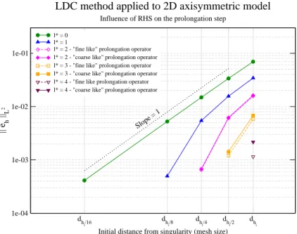
Figure 10 represents the relative discrete L2 error norm with respect to the distance between the real singularity and its approximation on the initial coarse mesh, and to the number of sub-grids. The “fine like” prolongation operator refers to the choice fk
l = fl0 whereas the “coarse like” prolongation operator refers to the choice fk
l = f
k−1
l . The
initial mesh step is hi= 327µm.
(a) Relative error for the displacement field according to the reference solu-tion
(b) Example of nested meshes - Areas of inter-est defined a priori (current mesh in black, zone to refined in green)
Figure 9: 2D axisymmetric test case - h0=hi
The first conclusion to be drawn is that, as expected, the mesh convergence of the global structured uniform meshes is of first-order with respect to the distance to the singularity. The second conclusion is that the two approaches concerning the prolongation operator conserve the order of convergence with respect to the local finest distance to the singu-larity until a stagnation appears. Indeed the same error level is obtained with a local refinement than with a global mono-grid of discretisation step equal to the local finest one. Thus, the LDC method converges as O(dhf ine), where dhf ine corresponds to the local distance to the singularity.
The two approaches lead to equivalent results before reaching the approximation error of the non-refined part. Then, the “fine like” prolongation operator seems to be a little more precise. However, both hypotheses need the same number of∧-cycles to converge, which means an equivalent CPU time.
dh i dh i/2 dh i/4 dh i/8 dh i/16
Initial distance from singularity (mesh size) 1e-04 1e-03 1e-02 1e-01 || e h ||L 2 l* = 0 l* = 1
l* = 2 - "fine like" prolongation operator l* = 2 - "coarse like" prolongation operator l* = 3 - "fine like" prolongation operator l* = 3 - "coarse like" prolongation operator l* = 4 - "fine like prolongation operator l* = 4 - "coarse like" prolongation operator
LDC method applied to 2D axisymmetric model
Influence of RHS on the prolongation step
Slope = 1
Figure 10: Influence of the prolongation operator on the intermediate levels - 2D(r,z) test case
The relative maximal error norms are reported in table 1.
Relative maximal error norm according to the prolongation operator H H H H H h0 l∗ 0 1 2 3 4 hi 1.14 10−1 5.83 10−2 ‘f’ : 2.69 10 −2 ‘f’ : 9.57 10−3 ‘f’ : 1.73 10−3 ‘c’ : 2.78 10−2 ‘c’ : 1.13 10−2 ‘c’ : 2.73 10−3 hi/2 5.77 10−2 2.72 10−2 ‘f’ : 1.05 10 −2 ‘f’ : 1.82 10−3 ‘c’ : 1.07 10−2 ‘c’ : 2.18 10−3 hi/4 2.62 10−2 9.71 10−3 ‘f’ : 1.17 10 −3 ‘c’ : 1.22 10−3 hi/8 9.65 10−3 9.42 10−4 hi/16 7.97 10−4
Table 1: Comparison between “fine like” ( ‘f’) and “coarse like” (‘c’) prolongation operator - 2D(r,z) test case - Relative maximal error norm
We can observe that the optimal convergence in O(dhf ine) is also reached before slow-ing down for fine error levels (< 1. 10−3). For example, the same error is obtained for
h0= hi/4 and l∗= 0 as for h0= hi/2 and l∗= 1 or h0= hi and l∗= 2. The behaviour of L2 and L∞ norms are similar. Here again, the “fine like” prolongation operator gives more accurate solution for expected fine error levels.
In order to also compare the solution obtained on the sub-grids for both approaches, the composite error norms are then looked at. The relative composite L2 error norms are plotted on figure 11 and the relative composite L∞error norms are detailed in table 2.
dh i dh i/2 dh i/4 dh i/8 dh i/16
Initial distance from singularity (mesh size) 1e-04 1e-03 1e-02 1e-01 || e h ||L 2 ,comp l* = 0 l* = 1
l* = 2 - "fine like" prolongation operator l* = 2 - "coarse like" prolongation operator l* = 3 - "fine like" prolongation operator l* = 3 - "coarse like prolongation operator l* = 4 - "fine like" prolongation operator l* = 4 - "coarse like" prolongation operator
LDC method applied to 2D axisymmetric model
Influence of RHS on the prolongation step
Slope = 1
Figure 11: Influence of the prolongation operator on the intermediate level - 2D(r,z) test case
Unlike the previous results, there is an important difference between the effects of the two types of prolongation operator. When the “coarse like” prolongation operator is used, the convergence remains in O(dhf ine) for both norms except for the finest error level. These results are consistent with the ones obtained by Anthonissen et al. [51]. The attained precision is then homogeneous from the finest to the coarsest grid. On the contrary, an early stagnation appears for the “fine like” prolongation operator. The more the initial mesh is coarse, the more the stagnation appears at early levels of refinement. So, in this case, the obtained results are far from the expected ones.
Relative composite maximal error norm according to the prolongation operator H H H H H h0 l∗ 0 1 2 3 4 hi 1.14 10−1 5.83 10−2 ‘f’ : 4.16 10 −2 ‘f’ : 3.83 10−2 ‘f’ : 3.67 10−2 ‘c’ : 2.78 10−2 ‘c’ : 1.15 10−2 ‘c’ : 2.79 10−3 hi/2 5.77 10−2 2.72 10−2 ‘f’ : 1.65 10 −2 ‘f’ : 1.12 10−2 ‘c’ : 1.10 10−2 ‘c’ : 2.23 10−3 hi/4 2.62 10−2 9.94 10−3 ‘f’ : 1.44 10 −3 ‘c’ : 1.24 10−3 hi/8 9.65 10−3 9.62 10−4 hi/16 7.97 10−4
Table 2: Comparison between “fine like” (‘f’) and “coarse like” (‘c’) prolongation operator - 2D(r,z) test case - Relative maximal composite error norm
In conclusion, both prolongation operators correct accurately the initial coarse mesh (whole structure) but only the “coarse like” operator brings accurate solution on local fine grids.
As we are interested in local values, in the sequel we will use by default the “coarse like” prolongation operator.
4.3. A posteriori error estimation
In this section, we are interested in automating the detection of areas of interest for two reasons. First, in the previous section we supposed that the stagnation was due to the discretisation error of the non-refined part. So, we aim to determine optimal refined zones in order to reach the expected precision (i.e. mono-grid error obtained for the same finest mesh step). Secondly, we are interested in moving singularities so we would like to have refinement zones adjusting automatically.
In this context, we chose to use the Zienkiewicz and Zhu (ZZ) a posteriori error estima-tor [38]. It is the most used error estimaestima-tor (e.g. [34, 58–61]) and its super-convergent patch recovery version [62, 63] gives really convincing performances in terms of precision over time consuming. Moreover, it can be easily performed and is already available in some industrial codes, as Code_Aster [64] or CAST3M [65]. This estimator has been proved theoretically for a linear one-dimensional problem [63]. Furthermore, it can be
expressed with the energy norm [66] which allows to extend it to any type of behaviour.
4.3.1. Presentation of Zienkiewicz and Zhu a posteriori error estimator
The ZZ estimator [38, 62, 63] consists in constructing a stress solution σ∗
h smoother than the FE one σh. The local estimator ηE,h on an element E is defined as:
ηE,h= k(σ∗h)E− (σh)Ek (5)
The element value is obtained from nodes values. For the FE stress σh, the values at the discretisation nodes are obtained by interpolating the values at the Gaussian points. To obtain the estimated stress σ∗
h, two methods are proposed by Zienkiewicz and Zhu: • The simplest and cheapest one [38] consists in averaging the value of the FE stress
σh on the elements surrounding the node. However, it is not very efficient for very coarse grids or for high-order polynomial basis.
• The second one, called “super convergent patch recovery” [62, 63], is based on patches, which are the union of several elements. On each patch, a high-order polynomial function is defined, which minimises the root mean square gap with re-spect to σhon so-called “super convergent” points (Gauss points in one dimensional problems). Then an average of each patch contribution is made to obtain σ∗
h. This method is a little bit more expensive but leads to better approximations.
In order to generate the LDC grids automatically in the maximum error zones, we decide to apply recursively the ZZ error estimator during the first prolongation step to obtain each next finer grid. At each level l, we hence refine the elements L of the grid Gl for which the local ZZ error e respects:
eL> α ( max K⊂Gl eK− min K⊂Gl eK) (6) with 0 ≤ α ≤ 1, α a given constant
The second-hand member of equation (6) enables to stop the refinement process when the solution is sufficiently smooth. We define a minimum number of elements required to build a new local sub-grid (typically 2D with D the space dimension). According to
the definition of ˚Aland Alin section 3.2.3, we also decide to enlarge the refinement zone in order to keep all the detected elements in the restriction zone ˚Al.
The more α is low, the more the number of elements to refine is important. In the sequel, we will look to an optimal value of α, that is to say the biggest value of α (i.e. minimal number of elements) leading to the expected error level.
With this strategy, we thus need less refinement levels than with a two-refinement com-parison error indicator [45, 67] where the level l is finally obtained thanks to the level l − 2.
4.3.2. Two-dimensional axisymmetric test case
On figure 12 the local error field calculated by the ZZ estimator is plotted, for an initial coarse mesh of uniform cells of mesh step 327µm.
Figure 12: Local error given by the ZZ a posteriori error estimator - 2D axisymmetric test case
Applying the detection formula, we can notice that the automatically detected areas (fig-ure 13, left) are not struct(fig-ured meshes. In order to keep advantages of regular struct(fig-ured meshes (natural tensor formulation, good convergence properties,. . . ), we decided to add some elements at each mesh to make them structured (figure 13, right) [29, 51].
On figure 14, we study the composite L2 error of the LDC method with respect to the refinement criterion α chosen for the ZZ automatic detection. The initial mesh step hi is the same than in section 4.2 (hi = 327µm).
Figure 13: Example of detected area (in red) and modification to obtain a structured mesh (in green) 0 0,1 0,2 0,3 0,4 0,5 0,6 0,7 0,8 0,9 1
Criterion alpha in the refinement process 1e-03 1e-02 1e-01 || e h || L 2 ,comp h 0 = hi , l * = 0 h 0 = hi , l * = 1 h 0 = hi , l * = 2 h 0 = hi , l * = 3 h 0 = hi/2 , l * = 0 h0 = hi/2 , l* = 1 h0 = hi/2 , l* = 2 h0 = hi/4 , l* = 0 h 0 = hi/4 , l * = 1 h 0 = hi/8 , l * = 0
LDC method applied to 2D axisymmetric model
Refinement criterion variation
Figure 14: Composite L2
error norm according to the criterion α used on the refinement process - 2D(r,z) test case
First, we see that the errors converge to the expected values. Moreover, there exists an optimal refinement criterion α for each expected error, independently to the number of sub-grids used and to the initial mesh size. Then a unique α depending only on the prescribed accuracy will be used for all refinement levels. However, a simple correlation between the optimal α and the expected error level does not appear clearly.
We can notice that for some error levels, large values of α lead to a smaller error for a local refinement than for a global one. This phenomenon has already been observed in the literature (see [28] for example). However, these values will not be retained since they do not lead to the asymptotic error value.
Using the obtained optimal α, the refinement zones are then larger than for the a priori study, see for example figure 15 and figure 9(b) that have the same initial mesh. That confirms that the stagnation observed before was related to a refinement area not suffi-ciently large for the expected precision.
Figure 15: Example of nested meshes - A posteriori error estimation with α = 0.15 - 2D axisymmetric test case (current mesh in black, zone to refined in green) - h0=hi
In this case, the optimal meshes (see figure 15) obtained seem to claim that the singu-larity effect is not very localised. However, if we look more deeply at figure 14, we can see that the asymptotic convergence is very slow. In an industrial context, we then could chose to be less strict. For example, within a margin of 10% on the expected accuracy, up to 50% of refined elements can be saved.
Using an optimal criterion, the mesh convergence of the LDC method is presented in table 3. Here again, both prolongation operators exposed in section 4.2 are compared to be sure that the previous conclusions are still valid with optimal refinement zones.
Relative composite maximal error norm according to the prolongation operator H H H H H h0 l∗ 0 1 2 3 4 hi 1.14 10−1 5.78 10−2 ‘f’ : 2.83 10 −2 ‘f’ : 1.10 10−2 ‘f’ : 2.04 10−3 ‘c’ : 2.63 10−2 ‘c’ : 9.66 10−3 ‘c’ : 7.95 10−4 hi/2 5.77 10−2 2.62 10−2 ‘f’ : 1.05 10 −2 ‘f’ : 2.04 10−3 ‘c’ : 9.67 10−3 ‘c’ : 7.95 10−4 hi/4 2.62 10−2 9.67 10−3 ‘f’ : 1.08 10 −3 ‘c’ : 7.95 10−4 hi/8 9.65 10−3 8.03 10−4 hi/16 7.97 10−4
Table 3: Comparison between “fine like” (‘f’) and “coarse like” (‘c’) prolongation operator - 2D(r,z) test case with ZZ optimal refinement criterion α - Relative maximal composite error norm
A stagnation of the composite maximal error norm begins to appear for the “fine like” prolongation operator while the optimal accuracy in O(dhf ine) is obtained for the “coarse like” prolongation operator. A better choice of the refinement zones has then a benefit effect on both versions of the LDC method. However, the “fine like” operator do not still correct completely the fine levels. In conclusion, the “fine like” version seems always stagnate before the “coarse like” version from a composite error norm point of view.
4.3.3. Two-dimensional plane strain test case
We then conduct the same study for the 2D plane strain test case (see section 2.4). In this case, the maximum error zone obtained thanks to the ZZ a posteriori error estimator is much more localised, even for an initial coarse mesh, see figure 16. This localisation can be explained by the fact that the structure is three times less stretched than in the previous study.
As the error field is very restricted and as a minimum number of detected elements is required to create a new level, the variation of the refinement criterion drives the number of sub-grids generated, except for the very fine meshes. The figure 17 shows the influence
Figure 16: Local error given by the ZZ a posteriori error estimator - 2D plane strain test case
of the refinement criterion on the LDC composite L2error norm. Here, the initial mesh step hi is 218µm.
As previously, for all cases, an optimal criterion can be obtained depending only on the expected error. However, the optimal values obtained per level of error are not similar to the ones obtained for the previous test case (see figure 14). The optimal values of α seem then also depend on the effect of the singularity under study. Results of the mesh convergence study in the maximal composite error norm with optimal α are reported in table 4 for both prolongation operators. An example of optimal nested sub-grids is given on figure 18.
For the “coarse like” operator, the method still converges as O(dhf ine), which is the expected order of convergence. It confirms that the geometry discretisation error is neg-ligible in front of the modelling error (see section 4.1).
As for the 2D(r,z) test case, an early stagnation appears for the “fine like” prolongation operator, especially for the initial coarsest mesh (h0= hi). Then, the error on the com-posite LDC grid is great deteriorated. For example, the error obtained for a simulation with h0 = hi and l∗ = 4 with the “fine like” operator leads to an error 40 times greater than for the “coarse like” operator.
0 0,1 0,2 0,3 0,4 0,5 0,6 0,7 0,8 0,9 1
Criterion alpha in the refinement process 1e-03 1e-02 1e-01 || e h || L 2 ,comp h0 = hi , l * = 0 h0 = hi , l * = 1 h0 = hi , l* = 2 h0 = hi , l * = 3 h0 = hi , l * = 4 h0 = hi/2 , l * = 0 h0 = hi/2 , l * = 1 h0 = hi/2 , l * = 2 h0 = hi/2 , l* = 3 h0 = hi/4 , l * = 0 h0 = hi/4 , l * = 1 h0 = hi/4 , l* = 2 h0 = hi/8 , l * = 0 h0 = hi/8 , l * = 1 h0 = hi/16 , l* = 0
LDC method applied to 2D plane strain model
Refinement criterion variation
Figure 17: Composite L2
error norm according to the criterion α used on the refinement process - 2D(r,θ) test case
Relative composite maximal error norm according to the prolongation operator H H H H H h0 l∗ 0 1 2 3 4 hi 1.75 10−1 8.67 10−2 ‘f’ : 8.40 10 −2 ‘f’ : 8.29 10−2 ‘f’ : 8.24 10−2 ‘c’ : 3.91 10−2 ‘c’ : 1.47 10−2 ‘c’ : 2.40 10−3 hi/2 8.61 10−2 3.94 10−2 ‘f’ : 1.59 10 −2 ‘f’ : 4.15 10−3 ‘c’ : 1.53 10−2 ‘c’ : 2.82 10−3 hi/4 3.93 10−2 1.52 10−2 ‘f’ : 3.03 10 −3 ‘c’ : 2.70 10−3 hi/8 1.52 10−2 2.68 10−3 hi/16 2.70 10−3
Table 4: Comparison between “fine like” (‘f’) and “coarse like” (‘c’) prolongation operator - 2D(r,θ) test case with optimal refinement criterion α - Relative maximal composite error norm
4.3.4. Conclusions
In conclusion, for both test cases, the refinement process has been successfully au-tomated by the use of the ZZ a posteriori error estimator. The performances of the
Figure 18: Example of nested meshes - A posteriori error estimation with an optimal α = 0.25 - 2D plane strain test case (current mesh in black, zone to refined in green) - h0=hi/2
combination of LDC and ZZ in terms of CPU time and memory space will be studied in section 5. As for any a posteriori error estimator, a criterion playing the role of threshold has to be set. We have seen that this criterion is of great importance in order to reach the optimal convergence. Even if this study has shown that for each test case the optimal criterion only depends on the expected error level, its value varies with the test case under study. For now, there is no simple correlation between the optimal criterion and the expected error independently of the singularity under consideration. However, for both studies, a ZZ criterion of 0.25 seems to offer a good compromise between precision and number of refined elements.
In the sequel, the ZZ a posteriori error estimator is always used to generate automatically the sub-grids. Optimal or compromise values of the refinement criterion α may be set. Moreover, the prolongation operator is always the “coarse like” one.
4.4. Extension to the three-dimensional test case
As said previously (see section 2.5), this test case gathers the two previous 2D phe-nomena on a three-dimensional geometry.
An a priori choice of the optimal refinement criterion α is not easy. Indeed, we saw in section 4.3 that it depends on the test case under study. Moreover, using the minimal value of the two criteria obtained in the previous 2D studies does not lead to the expected
results: it is too large for the biggest errors and too small for the smallest ones. Then, a convergence study according to the criterion α should be done again. As this sensi-bility study is very costly, especially in a 3D context, and according to the conclusions of section 4.3, we decide to conduct the mesh convergence study with a fixed criterion α = 0.25, which seems to be a good compromise for the two 2D studies.
The composite L2error norm between the reference solution and the LDC one is plotted on figure 19. In this case, d represents the initial distance between the real position of the two singularities intersection and its mesh approximation.
dh i dh i/2 dh i/4
Initial distance to singularity (mesh size) 0,001 0,01 0,1 || e h ||L 2,comp l*=0 l*=1 l*=2 l*=3 l*=4
LDC method applied to 3D model
ZZ with criterion α=0.25
Figure 19: Composite L2
error according to the mesh - 3D test case
The expected first-order convergence is reached for the uniform mono-grid solutions. However, more precise mono-grid solutions could not be obtained due to the important number of DoF implied.
The error improvement thanks to the local multi-grid refinement strategy remains true in a three-dimensional context since more precise solutions can easily be obtained. The LDC method applied to two crossed three-dimensional singularities converges as O(dhf ine) since the obtained errors are quasi optimal. Only the finest error presents a little gap
with the expected values. In this case the value α seems then a little to big. However the results obtained are really acceptable for a non user-dependent choice of α. This last study validates the a priori choice of α (0.25).
An example of refined meshes obtained with α = 0.25 can be seen on figure 20. The ZZ a posteriori error estimator well detect automatically the crossed singularities, and the finest meshes are very localised around the two singularities.
Figure 20: Example of optimal hierarchical meshes - ZZ a posteriori error estimator with α = 0.25 - 3D test case - h0=hi/2
As previously, the composite maximal relative error norm has also been studied, and the results are available in table 5.
kehkL∞,compwith α = 0.25 H H H H H h0 l∗ 0 1 2 3 4 hi 1.15 10−1 5.75 10−2 2.61 10−2 9.99 10−3 2.12 10−3 hi/2 5.64 10−2 2.60 10−2 1.00 10−2 1.91 10−3 hi/4 2.57 10−2 9.93 10−3 1.80 10−3
Table 5: 3D test case with refinement criterion α = 0.25 - Relative maximal composite error norm
Here again, the composite L2 and the L∞ error norms have the same behaviour and the convergence in O(dhf ine) is reached for the composite L∞ error norm. This LDC approach combined with the ZZ a posteriori error estimator seems really promising since for example, the maximal error norm is quite 100 times reduced adding 3 local levels of sub-grids to an initial uniform mesh of space step h0= hi.
5. Performances of the LDC method in an industrial context
5.1. Interest of sub-grids
We have previously shown that we can reach the same precision with a mono-grid uniform fine mesh or with a global coarse mesh and several local sub-grids as long as the local finest mesh size is the same. To optimise the ratio precision obtained over means (CPU time, memory space), we have studied the behaviour of the composite L2 error norm with respect to CPU time (see figure 21 for the 2D(r,θ) test case) as well as the behaviour of the composite L2error norm with respect to the total number of nodes (see figure 22 for the 2D(r,θ) test case). For both studies, the refinement process has been conducted with the optimal refinement criteria α obtained in the section 4.3.
From these figures, we can conclude that the more the precision expected is constraining, the more the use of an initial coarse mesh with many suitable sub-grids is advantageous, as well in terms of CPU time as in terms of memory space. These results are consistent with the ones obtained by Ramière [55] for the FIC method.
The same conclusion can be drawn for the 2D(r,z) test case or 3D test case.
5.2. Refinement ratio study
The LDC method applied on a FE discretisation is classically performed with a re-finement ratio of 2 (e.g. [31, 41, 51, 68]). Some studies, coupling the LDC method with a Finite Volume discretisation use a refinement ratio of 3 (e.g. [44]), for projection sim-plifications. But very few studies [28] compare several ratios of refinement on the same test case. As there is no theoretical limitation for the choice of the refinement ratio, we decide to compare the performance of the LDC method between a refinement ratio of 2
1e-02 1e-01 1 1e+01 1e+02 CPU time (s) 1e-04 1e-03 1e-02 1e-01 || e h || L 2 ,comp l* = 0 l* = 1 l* = 2 l* = 3 l* = 4
LDC method applied to 2D plane strain model
CPU time - ZZ with optimal refinement criterion
Figure 21: Composite error norm versus CPU time required for the simulation - 2D(r,θ) test case
1e+02 1e+03 1e+04 1e+05
Total number of nodes 1e-04 1e-03 1e-02 1e-01 || e h || L 2 ,comp l* = 0 l* = 1 l* = 2 l* = 3 l* = 4
LDC method applied to 2D plane strain model
Total number of nodes - ZZ with optimal refinement criterion
Figure 22: Composite error norm versus total number of nodes (sum of each level) - 2D(r,θ) test case
or of 4. The results for the 2D(r,θ) test case are presented in table 6.
Comparison between refinement ratio of 2 and 4 - h0= hi/2
l∗× r 2 × 2 1 × 4 4 × 2 2 × 4
kehkL2,comp 1.01 10−2 1.02 10−2 1.78 10−3 1.79 10−3
Sub-grids nodes 242 441 484 882
CPU time 0.04s 0.08s 0.11s 0.13s
Comparison between refinement ratio of 2 and 4 - h0= hi/16
l∗× r 2 × 2 1 × 4 4 × 2 2 × 4
kehkL2
,comp 1.65 10−3 1.68 10−3 1.04 10−4 1.32 10−4
Sub-grids nodes 242 441 638 1134
CPU time 2.42s 3.62s 2.65s 3.70s
Table 6: Comparison between a refinement ratio of 2 and 4 - 2D(r, θ) test case - Optimal refinement criterion
As expected by the theory, we obtain the same error levels for simulations made with two successive refinements of ratio 2 than with one refinement of ratio 4, even for small errors. Thus, the convergence as O(dhf ine) is conserved, whatever the refinement ratio used. Our LDC method with ZZ a posteriori error estimator is then really generic. The second conclusion to be drawn is that the use of a larger ratio reduces the number of sub-grids, but may imply the use of more extended grids and thus more nodes than necessary in some regions. In our case, as the zones of interest are more and more lo-calised, there are around twice more additional nodes for the ratio 4 than for the ratio 2 for the same error. Thus the refinement of 4 is not attractive in terms of total number of nodes for the test case under study. Moreover, this ratio also leads to slightly superior CPU time (up to 30% more) than a ratio of 2. However, as the considered CPU time are really small, this conclusion has to be confirmed on a more representative test case.
5.3. Comparison with a h-refinement method
The goal of this section is to compare the LDC method to the standard approach applied until now to simulate the cladding behaviour under irradiation. The standard meshes are mono-grid unstructured meshes refined around the singularities and can be
considered as meshes obtained with a global h-refinement method [6], see for example figure 23 left.
5.3.1. Two-dimensional plane strain test case
According to the conclusions of section 5.1, LDC seems efficient when a coarse initial mesh and a lot of local sub-grids are used. For this comparison, an initial mesh of size h0 = hi/2, with 1 to 7 sub-grids and a refinement ratio r = 2 is performed. As we set ourselves in an industrial position, the a priori refinement criterion α = 0.25 is set for all levels. Hence, this value allows to obtain a good compromise between the number of elements to refine and the error level reached (see conclusions of section 4.3). The meshes on figure 23 are examples of meshes used for this comparison. The composite L2 error norm against the CPU time is plotted on figure 24 for both approaches. Moreover, indications of total number of nodes are also given.
Figure 23: Example of meshes used in the comparison study: h-refined mesh (left) and LDC composite mesh with 4 sub-grids and refinement ratio of 2 (right)
We can notice that the LDC solver is really efficient. For errors about 1.10−2, com-putational times are approximately twice larger for the LDC method, but these times remain very small (∼ 0.05s). For smaller relative errors, less than 1.10−3, CPU times required for the LDC resolution are less than 2 times smaller than the one required for a h-refinement resolution.
Moreover, our method does not require any preliminary study in order to obtain a refined 36
1e-02 1e-01 1 CPU time (s) 1e-04 1e-03 1e-02 || e h ||L 2,comp LDC mesh - h0 = hi/2 - l * = 1 to 7 - r = 2 h-refinement - hmax = hi/2 - hmin = hi/4 to hi/128
LDC method applied to 2D plane strain model
Comparison with h-refinement - ZZ criterion with alpha = 0.25
341 nodes 972 nodes 4104 nodes 352 nodes 594 nodes 1232 nodes
Figure 24: CPU time and mesh size according to L2
error - 2D plane strain test case - Comparison between LDC solver and classical FE solver on locally refined mesh
mesh adapted to the singularity problem. As the generation of the sub-grids is automatic thanks to ZZ a posteriori error estimator, only a mesh size for the coarsest level and a refinement criterion are necessary. The use of the LDC method thus makes possible to save preprocessing times (mesh determination), that can be really important from an engineering point of view.
From a memory space saving point of view, the LDC method is also attractive. Indeed, even if extra informations are stored (boundary conditions on the levels, reversed matri-ces of stiffness, right-hand side,. . . ), each local grid is much smaller than an equivalent global refined grid. In particular the total number of nodes of all the sub-grids is far smaller than the number of nodes of the locally adapted grid used currently (2 times less nodes for an error about 1.10−3 and 4 times less for an error about 1.10−4, see figure 24).
To conclude, the LDC solver combined with a ZZ a posteriori error estimator seems very attractive. Indeed, even on a simple test case, which is a priori unfavourable for the LDC solver (2D, linear elasticity, precise and quick solving on a mono-grid stretched mesh), the LDC tool enables us to save CPU time and memory space for a prescribed accuracy
of the solution.
5.3.2. Three-dimensional test case
The comparison between the adaptive h-refinement method and the LDC solver has been also made for the three-dimensional test case, see table 7.
Mesh kehkL∞,comp CPU time Number of nodes
LDC, α = 0.25
2.61 10−2 143 s total: 42813
h0= hi, l∗= 2 max per level: 34121
h-refinement
2.35 10−2 659 s 78819
hmax= hi
Table 7: Comparison between LDC and h-refinement resolution - 3D model
These results are still really encouraging. Indeed, for a maximum error level about 2%, we obtain interesting CPU time and memory space: the LDC solver enables us to save 46% of the total number of nodes and 78% of CPU time. Furthermore, it should be noticed that for the LDC method, the number of nodes represents the sum of the nodes on all the grids. Hence, the most costly level has 34121 nodes which is equivalent to 57% of the nodes of the h-refinement mesh. Thus, we will be later limited by the local finest mesh step acceptable for the triangularisation of the stiffness matrix. In particular, that means that an important limitation of the industrial simulation is then pushed back. These performances could be more improved by using a domain decomposition method on patch elements [51].
To conclude, for the industrial test cases under study, the use of the LDC method is much more attractive than the global h-refinement. Indeed, the same given error is obtained in less CPU time and with less DoF, in 2D as well as in 3D simulations. These results give confidence in the use of the LDC solver for more complex studies.
6. Conclusions and prospects
The use of the Local Defect Correction (LDC) multi-level method in a linear struc-tural mechanics context has been verified. Some strategies have been tested to reach the best performances in an industrial context. The method proposed here is an efficient tool
based on a “black-box” solver concept. By this way, it can be easily performed in any ex-isting industrial software. Moreover, by construction, the LDC method can be combined with any a posterior error estimator in order to automate the local sub-grids generation. In this paper, the classical and widely used Zienkiewicz and Zhu error estimator based on the super convergent patch recovery has been chosen. For non-academic test cases, in particular 3D crossed-singularities problems, the resulting local multi-grid solver leads to the same precision as the standard h-refinement method but with a important gain in terms of CPU time and memory space.
These first results give confidence in the use of a LDC solver for more complex structural mechanics behaviour, such as non-linear path-dependent behaviour. Actually, this tech-nique has already been successfully extended to “one-time-step” non linear behaviour, see Barbié et al. [69].
References
[1] S. Ghosh, S. Manna, r-adapted arbitrary Lagrangian-Eulerian finite-element method in metal-forming simulation, Journal of Materials Engineering and Performance 2 (2) (1993) 271–282. [2] W. Cao, W. Huang, R. Russell, Comparison of two-dimensional r-adaptive finite element methods
using various error indicators, Mathematics and Computers in Simulation 56 (2001) 127–143. [3] T. Strouboulis, K. Haque, Recent experiences with error estimation and adaptivity - 2. Error
esti-mation for h-adaptive approxiesti-mations on grids of triangles and quadrilaterals, Computer Methods in Applied Mechanics and Engineering 100 (3) (1992) 359–430.
[4] T. Belytschko, M. Tabbara, H-adaptive finite-element methods for dynamic problems, with em-phasis on localization, International Journal for Numerical Methods in Engineering 36 (24) (1993) 4245–4265.
[5] J. Fish, S. Markolefas, Adaptive global-local refinement strategy based on the interior error-estimatesd of the h-method, International Journal for Numerical Methods in Engineering 37 (5) (1994) 827–838.
[6] P. Díez, A. Huerta, A unified approach to remeshing strategies for finite element h-adaptivity, Computer Methods in Applied Mechanics and Engineering 176 (1999) 215–229.
[7] G. Bessette, E. Becker, L. Taylor, D. Littlefield, Modeling of impact problems using an h-adaptive, explicit lagrangian finite element method in three dimensions, Computer Methods in Applied Me-chanics and Engineering 192 (2003) 1649–1679.
[8] I. Babuska, M. Suri, The optimal convergence rate of the p-version of the finite-element method, SIAM Journal on Numerical Analysis 24 (4) (1987) 750–776.
[9] F. Barros, S. Proenca, C. de Barcellos, Generalized finite element method in structural nonlinear analysis - a p-adaptive strategy, Computational Mechanics 33 (2) (2004) 95–107.
[10] A. Düster, E. Rank, The p-version of the finite element method compared to an adaptive h-version for the deformation theory of plasticity, Computer Methods in Applied Mechanics and Engineering 190 (2001) 1925–1935.
[11] J. Fish, The s-version of the finite-element method, Computers and Structures 43 (3) (1992) 539– 547.
[12] Z. Yue, D. Robbins, Adaptive superposition of finite element meshes in elastodynamic problems, International Journal for Numerical Methods in Engineering 63 (11) (2005) 1604–1635.
[13] W. Sun, N. Zamani, An adaptive h-r boundary element algorithm for the Laplace equation, Inter-national Journal for Numerical Methods in Engineering 33 (3) (1992) 537–552.