HAL Id: cea-02388704
https://hal-cea.archives-ouvertes.fr/cea-02388704
Submitted on 2 Dec 2019HAL is a multi-disciplinary open access archive for the deposit and dissemination of sci-entific research documents, whether they are pub-lished or not. The documents may come from teaching and research institutions in France or abroad, or from public or private research centers.
L’archive ouverte pluridisciplinaire HAL, est destinée au dépôt et à la diffusion de documents scientifiques de niveau recherche, publiés ou non, émanant des établissements d’enseignement et de recherche français ou étrangers, des laboratoires publics ou privés.
An analytical relation for the void fraction distribution
in a fully developed bubbly flow in a vertical pipe
O. Marfaing, M. Guingo, J. Laviéville, G. Bois, N. Mechitoua, N. Mérigoux, S.
Mimouni
To cite this version:
O. Marfaing, M. Guingo, J. Laviéville, G. Bois, N. Mechitoua, et al.. An analytical relation for the void fraction distribution in a fully developed bubbly flow in a vertical pipe. Chemical Engineering Science, Elsevier, 2016, 152, pp.579-585. �10.1016/j.ces.2016.06.041�. �cea-02388704�
CHEMICAL ENGINEERING SCIENCE
An analytical relation for the void fraction distribution in a
fully developed bubbly flow in a vertical pipe
O. Marfaing a,*, M. Guingo b, J. Laviéville b, G. Bois a, N. Méchitoua b, N. Mérigoux b,S. Mimouni b
a. Den-Service de thermo-hydraulique et de mécanique des fluides (STMF), CEA, Université Paris-Saclay, F-91191, Gif-sur-Yvette, France
b. Electricité de France R&D Division, 6 Quai Watier, F-78400 Chatou, France * Corresponding author : olivier.marfaing@cea.fr
Keywords: two-fluid model, analytical relation, verification, wall force, lift force, dispersion force, drag force, NEPTUNE_CFD
Summary
The problem of a steady, axisymmetric, fully developed adiabatic bubbly flow in a vertical pipe is studied analytically with the two-fluid model. The exchange of momentum between the phases is described as the sum of drag, lift, wall and dispersion contributions, with constant coefficients.
Under these conditions, we are able to derive an analytical relation between the void fraction, the liquid velocity, and the pressure profiles. This relation is valid independently of the turbulence model in the liquid phase – here, a k-ε model is used – and can serve as a verification case for multiphase flow codes.
The analytical void fraction profile vanishes at the wall, as a result of the balance between dispersion and wall forces. This profile is illustrated by calculations performed for upward and downward bubbly flows with the NEPTUNE_CFD code.
1. Introduction
Multiphase flows are encountered in many industrial situations related to nuclear or chemical engineering. In order to address the growing need for simulations, the models and numerical schemes used in industrial codes need to be properly verified and validated [1,2].
One of the difficulties in the verification of multiphase flow solvers is the coupling between phases, which makes the search for analytical solutions more difficult, when compared to single-phase flows.
In this paper, we consider the problem of a (statistically) steady, axisymmetric, fully developed adiabatic bubbly flow in a vertical pipe. In the two-fluid formalism [5,6,7], a balance equation is written for the mass and momentum of each phase, and the coupling between the liquid and the gas is accounted for by an interfacial exchange term in the momentum balances. In order to perform an analytical study, simplifying assumptions are introduced:
(i) the flow is statistically steady and fully developed. Variations in the gas and liquid densities are therefore neglected.
(ii) the bubbles all have the same diameter, denoted by db.
(iii) the interfacial exchange term is the sum of four contributions: drag, lift, wall forces, and a dispersion effect proportional to the void fraction gradient. The expressions of these forces (see Section 2) are assumed to have constant coefficients. Note that the virtual mass effects do not play a role in a developed steady flow.
Under these conditions, we are able to give an analytical expression for the void fraction profile, as a function of the liquid velocity and pressure profiles. In particular, we show that the compensation between wall and dispersion forces causes the void fraction to vanish at the wall. Note that this equation is valid independently of the chosen turbulence model. Of course, because of this generality, it is not possible to give a complete analytical solution, that is to express the velocity and pressure profiles as functions of the independent variables x, y, z only. In view of this generality, this analytical expression can serve as a verification case for multiphase flow codes.
In Section 3, calculations are performed for upward and downward bubbly flows with the NEPTUNE_CFD code [3,4]. NEPTUNE_CFD is a Computational Multi-Fluid Dynamics code dedicated to the simulation of multiphase flows, primarily targeting nuclear thermal-hydraulics applications, such as the departure from nuclear boiling (DNB) or the two-phase Pressurized Thermal Shock (PTS). It has been developed within the joint NEPTUNE R&D project (AREVA, CEA, EDF, IRSN) since 2001.
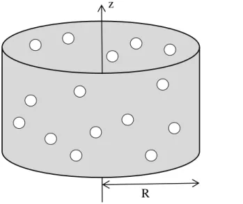
We consider an adiabatic bubbly flow in a vertical cylindrical pipe with radius R (see Fig 1). The flow is assumed to be (statistically) steady, axisymmetric, and fully developed. In particular, no phase change occurs, and the variations in the gas and liquid densities are neglected.
z
𝑔⃗
R
Fig 1 – bubbly flow in a vertical pipe
In all what follows, we denote with subscript g (resp. l) quantities relating to the gas (resp. liquid) phase. For k = g or l, the mass balance for phase k writes:
𝜕
𝜕𝑡(𝛼𝑘𝜌𝑘) + ∇. (𝛼𝑘𝜌𝑘𝑉⃗⃗𝑘) = 0 (1) Because the flow is steady and fully developed, it follows that the radial component of velocity 𝑉⃗⃗𝑘 is 0, while its axial component only depends on r. So we can write
𝑉⃗⃗𝑘= 𝑉𝑘(𝑟)𝑒⃗𝑧 (2)
Now we come to the momentum balance. For the derivation of our analytical relation, the momentum balance is written only for the gas phase, in the radial and axial directions. In particular it means we need no specific assumption on turbulence in the liquid phase.
Because the viscosity and density ratios 𝜇𝑔⁄ , 𝜇𝑙 𝜌𝑔⁄ are small, we can neglect viscous and 𝜌𝑙 Reynolds stresses for the gas phase, an assumption that is widely used in theoretical studies, see e.g. [5 Chp 11, 8, 9].
𝜕
𝜕𝑡(𝛼𝑔𝜌𝑔𝑉⃗⃗𝑔) + ∇. (𝛼𝑔𝜌𝑔𝑉⃗⃗𝑔𝑉⃗⃗𝑔) = −𝛼𝑔∇𝑃⃗⃗⃗⃗⃗⃗ + 𝛼𝑔𝜌𝑔𝑔⃗ + 𝑀⃗⃗⃗𝑔 (3) In the above equation, 𝑀⃗⃗⃗𝑔 stands for the interfacial momentum exchange term. The modeling of this term is now discussed. Then, in Section 3, we write the axial and radial components of Equation (3) and derive the analytical relation between the void fraction and the liquid
velocity and pressure profiles.
As explained in the introduction, the interfacial momentum transfer term 𝑀⃗⃗⃗𝑔 is written as the sum of four contributions: drag, lift, wall, and dispersion force, all of which have constant coefficients.
Because of (2), it can be seen that material derivatives of the form 𝜕𝑡𝜕 𝑉⃗⃗𝑘+ (𝑉⃗⃗𝑘. ∇). (𝑉⃗⃗𝑘) cancel, so virtual mass contribution is zero.
In the following, we denote by
𝑈⃗⃗⃗𝑅 ≡ 𝑉⃗⃗𝑔− 𝑉⃗⃗𝑙 (4)
the relative velocity between the phases. The drag force
The contribution of the drag force is expressed in the following way: 𝑀⃗⃗⃗𝑔𝐷 = −34𝛼𝑔𝜌𝑙𝐶𝐷
𝑑𝑏|𝑈⃗⃗⃗𝑅|𝑈⃗⃗⃗𝑅 (5)
where db stands for the (constant) bubble diameter, and CD is the drag coefficient, which is
here assumed to be constant. The dispersion force
The dispersion force, proportional to the void fraction gradient, results in the migration of bubbles from high to low void fraction regions. This effect is interpreted as the fluctuating part of other forces, in the averaging process leading to the two-fluid model [5, Chp 7]. Several models have been developed [10, 11, 12, 13, 14] in the literature to take into account this diffusive effect. In [10], Davidson expresses it as the product of the drag function and an apparent mean drift velocity of the liquid relative to the gas phase:
𝑀⃗⃗⃗𝑔 𝑑𝑖𝑠𝑝
= −34𝛼𝑙𝜌𝑙𝐶𝑑𝐷
𝑏|𝑈⃗⃗⃗𝑅|𝐷eff∇𝛼⃗⃗⃗⃗⃗⃗⃗⃗ 𝑔
where Deff is an effective bubble dispersion coefficient, considered as constant. The model proposed by Krepper et al. [13] uses the liquid turbulent viscosity 𝜇𝑙𝑇 𝑀⃗⃗⃗𝑔 𝑑𝑖𝑠𝑝 = −34𝐶𝐷 𝑑𝑏𝜇𝑙 𝑇|𝑈⃗⃗⃗ 𝑅|∇𝛼⃗⃗⃗⃗⃗⃗⃗⃗ 𝑔
In [14], Laviéville et al. express the transfer term as a function of the liquid turbulent kinetic energy:
𝑀⃗⃗⃗𝑔 𝑑𝑖𝑠𝑝
= −𝐺𝑇𝐷𝜌𝑙𝑘𝑙∇𝛼⃗⃗⃗⃗⃗⃗⃗⃗ 𝑔
where GTD is a function of the drag, lift and virtual mass coefficients.
In this part we will adopt the following model, very close to Davidson’s expression 𝑀⃗⃗⃗𝑔𝑑𝑖𝑠𝑝 = −34𝜌𝑙𝐶𝐷
𝑑𝑏|𝑈⃗⃗⃗𝑅|𝐷eff∇𝛼⃗⃗⃗⃗⃗⃗⃗⃗ 𝑔 (6)
where we simply removed the dependence upon the liquid volume fraction (which can be assumed to be approximately 1 in the case of low void fraction). Again, the bubble dispersion coefficient 𝐷eff is assumed to be constant.
The lift force
The contribution of the lift force is expressed in the following way: 𝑀⃗⃗⃗𝑔𝐿 = −𝛼𝑔𝜌𝑙𝐶𝐿𝑈⃗⃗⃗𝑅× (rot⃗⃗⃗⃗⃗⃗ 𝑉⃗⃗𝑙) (7)
where the lift coefficient CL is here assumed to be constant.
The wall force
The wall force is close to Antal’s model [9]: 𝑀⃗⃗⃗𝑔 𝑊 = 2𝛼𝑔𝜌𝑙|𝑈𝑅,||| 2 𝑑𝑏 Max [0, 𝐶𝑊1+ 𝐶𝑊2 𝑑𝑏 2𝑦] 𝑛⃗⃗𝑊 (8)
where 𝐶𝑊1 = −0.1 and 𝐶𝑊2 = 0.147 are taken as constants, y stands for the distance to the wall, and 𝑈𝑅,|| denotes the component of the relative velocity parallel to the wall.
With this expression, the bubbles are pushed away from the wall if they are at a distance 𝑦 < − 𝐶𝑊2
2𝐶𝑊1𝑑𝑏.The Max function guarantees that they are not attracted if 𝑦 > −
𝐶𝑊2
2𝐶𝑊1𝑑𝑏.
3. The analytical relation
3.1. Momentum balance for the gas phase in the axial and radial directions
Using equations (2), (4), (5), (6), (7) and (8), the gas phase momentum balance (3) is now projected in axisymmetric cylindrical coordinates.
From equation (2), the left hand side of the momentum balance, that is, quantity 𝜕
𝜕𝑡(𝛼𝑔𝜌𝑔𝑉⃗⃗𝑔) + ∇. (𝛼𝑔𝜌𝑔𝑉⃗⃗𝑔𝑉⃗⃗𝑔), is zero. Axial direction
The flow being steady and fully-developed, the axial momentum equation reduces to 0 = −𝛼𝑔𝜌𝑔𝑔 − 𝛼𝑔𝜕𝑃𝜕𝑧−34𝛼𝑔𝜌𝑙𝐶𝐷
𝑑𝑏|𝑈𝑅|𝑈𝑅 (9)
Simplifying by the void fraction, it follows that the relative velocity is constant and uniform in the pipe, with value given by:
|𝑈𝑅|𝑈𝑅 = −3𝜌4𝑑𝑏
𝑙𝐶𝐷(𝜌𝑔𝑔 +
𝜕𝑃 𝜕𝑧)
For bubbly flows, the main phase is the liquid. So the axial pressure gradient is of the order of magnitude of the hydrostatic pressure gradient for a liquid column:
𝜕𝑃
𝜕𝑧 ~ − 𝜌𝑙𝑔
Because the liquid density is much larger than the gas density, the relative velocity is seen to be positive, with value
𝑈𝑅 = √3𝜌4𝑑𝑏
𝑙𝐶𝐷(−
𝜕𝑃
𝜕𝑧− 𝜌𝑔𝑔) (10) Radial direction
The projection of equation (3) onto the radial direction writes: 0 = −𝛼𝑔𝜕𝑃𝜕𝑟− 𝛼𝑔𝐶𝐿𝜌𝑙𝑈𝑅𝜕𝑉𝜕𝑟𝑙− 2𝛼𝑔𝜌𝑙|𝑈𝑅| 2 𝑑𝑏 𝐹𝑊− 3 4𝜌𝑙 𝐶𝐷 𝑑𝑏|𝑈𝑅|𝐷eff 𝜕𝛼𝑔 𝜕𝑟 (11) where we have set:
𝐹𝑊 = Max [0, 𝐶𝑊1+ 𝐶𝑊22(𝑅−𝑟)𝑑𝑏 ] (12) Rearranging terms in (11), and simplifying by the void fraction, it follows:
1 𝛼𝑔 𝜕𝛼𝑔 𝜕𝑟 = − 4 3 𝑑𝑏 𝐶𝐷𝜌𝑙|𝑈𝑅|𝐷eff 𝜕𝑃 𝜕𝑟− 4 3 𝐶𝐿𝑑𝑏 𝐶𝐷𝐷eff 𝜕𝑉𝑙 𝜕𝑟 − 8 3 |𝑈𝑅| 𝐶𝐷𝐷eff 𝐹𝑊 (13)
From (10), 𝑈𝑅 is a constant, and (13) can then be integrated analytically.
We begin by rewriting (13) in non-dimensional form. As in (8), 𝑦 = 𝑅 − 𝑟 denotes the distance to the wall. Let
𝑦∗ ≡2𝑦
𝑑𝑏 (14)
𝑉𝑙∗ ≡ 𝑉𝑙
|𝑈𝑅| (15)
be the non-dimensional liquid velocity, and 𝐷eff∗ ≡ 34𝐶𝐷𝐷eff
|𝑈𝑅|𝑑𝑏 (16)
be the non-dimensional bubble dispersion coefficient. (13) can be rewritten: 1 𝛼𝑔 𝜕𝛼𝑔 𝜕𝑦∗ = − 1 𝜌𝑙|𝑈𝑅|2𝐷eff ∗ 𝜕𝑃 𝜕𝑦∗− 𝐶𝐿 𝐷eff ∗ 𝜕𝑉𝑙∗ 𝜕𝑦∗ + 𝐹𝑊 𝐷eff ∗ (17) and 𝐹𝑊= Max [0, 𝐶𝑊1+𝐶𝑊2 𝑦∗ ]. On the domain 0 < 𝑦∗< −𝐶𝑊2 𝐶𝑊1, equation (17) writes: 1 𝛼𝑔 𝜕𝛼𝑔 𝜕𝑦∗ = − 1 𝜌𝑙|𝑈𝑅|2𝐷eff ∗ 𝜕𝑃 𝜕𝑦∗− 𝐶𝐿 𝐷eff ∗ 𝜕𝑉𝑙∗ 𝜕𝑦∗ + 1 𝐷eff ∗(𝐶𝑊1+ 𝐶𝑊2 𝑦∗ ) (18)
and integrates into
𝛼𝑔 = 𝐵(𝑦∗)𝐶𝑊2⁄𝐷eff ∗exp (𝐶𝑊1 𝐷eff ∗𝑦 ∗) exp (− 𝐶𝐿 𝐷eff ∗𝑉𝑙 ∗) exp (− 𝑃−𝑃|𝑦=0 𝜌𝑙|𝑈𝑅|2𝐷eff ∗) (19)
where B is a constant. In the last factor, 𝑃|𝑦=0 is the pressure at the wall. Because the flow is developed, the pressure difference 𝑃 − 𝑃|𝑦=0 is independent on the axial coordinate z. So the use of the pressure difference in the last factor of (19), instead of pressure 𝑃, ensures that B is independent on z as well. Similarly, for 𝑦∗ > −𝐶𝑊2 𝐶𝑊1 , we have 𝛼𝑔 = 𝐵′ exp (−𝐷𝐶𝐿 eff ∗𝑉𝑙 ∗) exp (− 𝑃−𝑃|𝑦=0 𝜌𝑙|𝑈𝑅|2𝐷eff ∗) (20)
where B’ is another constant.
Expressions (19) and (20) have to connect continuously at 𝑦∗ = −𝐶𝑊2
𝐶𝑊1 . So let Y* be defined
by:
𝑌∗ ≡ min (−𝐶𝑊2
𝐶𝑊1 ; 𝑦
∗) (21) The following expression is now valid for all y*: 𝛼𝑔 = 𝐵(𝑌∗) 𝐶𝑊2 𝐷eff ∗ ⁄ exp (𝐶𝑊1 𝐷eff ∗𝑌 ∗) exp (− 𝐶𝐿 𝐷eff ∗𝑉𝑙 ∗) exp (− 𝑃−𝑃|𝑦=0 𝜌𝑙|𝑈𝑅|2𝐷eff ∗) (22)
with B a constant, which can be determined, knowing for instance the void fraction at the center of the pipe.
3.2. Discussion
Equation (22) shows that the void fraction profile results from an equilibrium between lift, wall and dispersion forces.
The effect of the lift force, expressed in the factor exp (− 𝐶𝐿
𝐷eff ∗𝑉𝑙
∗), is seen to depend on the sign of the liquid velocity and the lift coefficient. Assume the latter is positive. For upward flows, 𝑉𝑙∗ is maximum at the center of the pipe, and minimum at the wall. So the bubbles are pushed towards the wall. On the opposite, in downward flows, 𝑉𝑙∗ is negative, and the bubbles accumulate in the central region of the pipe, where the liquid velocity is minimum.
Due to the wall force, the void fraction is zero at the wall. Coming back to equation (18), we can thus see that, when y* tends to zero, the dominant terms in the radial momentum equation are dispersion and wall forces, which counterbalance each other. This can be seen from equation (13), after simplification by the void fraction: because the diffusion coefficient Deff does not vanish at the wall, the wall force term 𝐹𝑊, which goes to infinity when y* tends to zero, can be “absorbed” by the term proportional to 𝐷eff
𝛼𝑔
𝜕𝛼𝑔
𝜕𝑟. Note that this counterbalancing between dispersion and wall force can still take place if coefficient Deff vanishes at the wall, for instance if Deff decreases slower than 𝛼𝑔(eg as 𝛼𝑔𝑠 with parameter s<1). This issue does not seem to have been widely explored yet. Many models of dispersion force from the
literature are derived in regions far away from the walls, where some gradients (of velocity or velocity covariance) can be neglected. We believe the derivation of dispersion models specific to near-wall regions would be an important topic of investigation.
In the next section, the discussion is illustrated by calculations performed with the NEPTUNE_CFD code.
4. Numerical calculations
The problem being axisymmetric, the computational domain is limited to a sector of cylinder with an opening angle of 10°. The radius R of the pipe is set to 19 mm. The meshes used are uniform in the radial direction, with 1 cell both in the axial and orthoradial directions. Symmetry boundary conditions are imposed on the azimuthal planes.
In order to compute a developed solution, periodic boundary conditions are imposed on the top and bottom sections of the pipe. The pressure gradient is imposed as a volumetric source term. In order to compute a steady solution, calculations are run with the transient solver of NEPTUNE_CFD until the void fraction profile is seen to be steady. In most cases, the void fraction profiles reach a steady state after 15 s, and the calculations are stopped at 20 s. The liquid (resp. gas) density is set to 1000 kg/m3 (resp. 1 kg/m3). The liquid (resp. gas) dynamic viscosity is set to 10-3 kg.m-1.s-1 (resp. 10-5 kg.m-1.s-1). The bubble diameter is 2.5 mm. Turbulence in the liquid phase is accounted for with a k-ε model. The drag, lift and non-dimensional dispersion coefficients are taken as CD = CL = Deff* = 0.1.
In all cases below, the theoretical profile given by relation (22) is computed with the numerical velocity and pressure fields calculated by the solver. As explained in the end of Section 3.1, the factor B in (22) is determined by the numerical value of the void fraction at radial position r = 0.
3.1. Upward bubbly flow
In this calculation, the imposed pressure gradient 𝜕𝑃 𝜕𝑧⁄ is set to -9712 Pa.m-1, slightly below the hydrostatic pressure gradient. At initial time, t = 0, the void fraction is uniform with value 0.02. Two meshes were used, respectively with 50 and 100 cells in the radial direction. The radial void fraction profile is displayed in figure 2 for both meshes.
Fig 2 – void fraction profile for an upward flow. The red (resp. blue) line corresponds to the calculation with 50 cells (resp. 100).
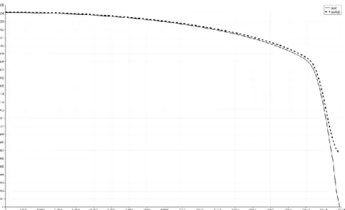
The void fraction profile obtained with 100 cells can therefore be considered as converged. In figure 3, we compare the profile obtained in the 100-cell calculation to the analytical one given by application of equation (22).
Fig 3 – Void fraction profile for the upward bubbly flow. The dashed line stands for the numerical solution computed with 100 cells, while the solid line results from formula (22).
The analytical and numerical curves are seen to be close to each other. As discussed in Section 3.2, in this upward bubbly flow configuration, bubbles accumulate in the near-wall region: the void fraction profile is seen to be almost uniform in the center of the pipe, to reach a maximum at a distance of the order of one bubble radius from the wall, and then to decrease at the wall.
3.2. Downward bubbly flow
The pressure gradient 𝜕𝑃 𝜕𝑧⁄ is now set to -9515 Pa.m-1, slightly above the hydrostatic pressure gradient. At initial time, t = 0, the void fraction field is uniform with value 0.02. In figure 4, we display the analytical void fraction profile and the numerical profile obtained in the 100-cell calculation.
Fig 4 – Void fraction profile for the downward bubbly flow. The dashed line stands for the numerical solution computed with 100 cells, while the solid line results from formula (22).
Both curves are in good agreement with each other. Unlike the upward bubbly flow case, the void fraction is maximum at the center of the pipe and decreases with the radial position. This decrease is slow in the bulk of the flow. At a distance of approximately one bubble radius, the void fraction decreases more rapidly, to tend to zero at the wall.
4. Conclusion
In this work, we perform an analytical study of the problem of a statistically steady axisymmetric fully developed adiabatic bubbly flow in a vertical pipe. The analysis is conducted with the two-fluid formalism.
The interfacial momentum transfer 𝑀⃗⃗⃗𝑔 is modeled as the sum of four contributions: drag, dispersion, lift, and wall forces, with constant coefficients.
We use the gas momentum balance equation to derive an analytical expression for the void fraction as a function of the liquid velocity and pressure profiles. Since the liquid momentum balance equation is not used, our analytical relation is valid independently of the model chosen for liquid turbulence. In view of this generality, it can serve as a verification case for multiphase flow codes.
We show that the void fraction profile results from an equilibrium between lift, wall and dispersion forces.
The effect of the lift force is seen to depend on the sign of the liquid velocity. If the lift coefficient is positive, upward flows push the bubbles towards the wall, whilst downward flows cause them to accumulate in the central region of the pipe, where the liquid velocity is (negative and) minimum. This behavior is illustrated by calculations with the
NEPTUNE_CFD code.
Near the wall, the dominant effects are dispersion and wall forces, which counterbalance each other, and the void fraction tends to zero.
It must be noted, however, that many models of dispersion force from the literature are derived in regions far away from the walls, where gradients (of velocity or velocity
covariance) can be neglected. We believe the derivation of dispersion models specific to near-wall regions would be an important topic of investigation.
Acknowledgements
This work has been achieved in the framework of the NEPTUNE project, financially
supported by CEA (Commissariat à l’Energie Atomique), EDF (Electricité de France), IRSN (Institut de Radioprotection et de Sûreté Nucléaire) and AREVA-NP.
Notations
B constant in equation (22), determined from the knowledge of the average void fraction
over a cross-section
CD drag coefficient
CL lift coefficient
CW1 , CW2 wall coefficients
db bubble diameter (m)
Deff effective dispersion coefficient (m2/s)
Deff * non-dimensional effective dispersion coefficient
g gravity (m2/s)
Mg interfacial momentum exchange term (Pa/m)
r radial coordinate (m) R radius of the pipe (m)
UR relative velocity (m/s)
Vk velocity of phase k (m/s)
y distance to the wall (m)
y* non-dimensional distance to the wall Y* non-dimensional quantity defined by (21) z axial coordinate (m)
Greek letters
αk volume fraction of phase k
μk viscosity of phase k ρk density of phase k Subscripts k k-th phase g gas phase l liquid phase Mathematical operators
sgn(x) sign of x : equals 1 for x > 0 and -1 for x < 0. References
1. M. Z. Podowski, Model verification and validation issues for multiphase flow and heat
transfer simulation in reactor systems, Keynote Lecture, CFD4NRS-5 conference, September
9-11 2014, Zurich, Switzerland.
2. C. Boyd, Perspectives on CFD analysis in nuclear reactor regulation, Keynote Lecture, CFD4NRS-5 conference, September 9-11 2014, Zurich, Switzerland.
3. A. Guelfi et al, NEPTUNE: A New Software Platform for Advanced Nuclear Thermal
4. M. Guingo et al, Recent Advances in Modeling and Validation of Nuclear
Thermal-Hydraulics Applications with NEPTUNE_CFD, Proceedings of the ICAPP conference, Nice,
3-6 May 2015.
5. C. Morel, Mathematical Modeling of Disperse Two-Phase Flows, Springer, 2015, DOI: 10.1007/978-3-319-20104-7.
6. M. Ishii, T. Hibiki, Thermo-Fluid Dynamics of Two-Phase Flows, Springer, 2010, DOI: 10.1007/978-1-4419-7985-8.
7. D.A. Drew, S. L. Passman, Theory of Multicomponent Fluids, Springer, 1999, ISBN 0-387-98380-5
8. O. E. Azpitarte, G. C. Buscaglia, Analytical and numerical evaluation of two-fluid model
solutions for laminar fully developed bubbly two-phase flows, Chemical Engineering Science,
2003, Vol 58, pp 3765 – 3776
9. S. P. Antal, R. T. Lahey Jr, J. E. Flaherty, Analysis of phase distribution in fully developed
laminar bubbly two-phase flow, International Journal of Multiphase Flow, Vol 17 (5), pp
635-652.
10. M. R. Davidson, Numerical calculations of two-phase flow in a liquid bath with bottom
gas injection: The central plume, Appl. Math. Modelling, 1990, Vol 14, pp 67 -76.
11. M. Lopez de Bertodano, Two-Fluid Model for Two-Phase Turbulent Jet, Nuclear Engineering and Design, 1998, Vol 179, 11, pp 65-74
12. A. D. B. Burns, T. Grank, I. Hamill, J. M. Shi, The Favre Averaged Drag Model for
Turbulent Dispersion in Eulerian Multi-Phase Flows, 5th International Conference on Multiphase Flows ICMF, Yokohama, Japan, 2004.
13. E. Krepper, D. Lucas, J. M. Shi, H. M. Prasser, Simulations of FZR adiabatic air-water
data with CFX-10, Nuresim European project, D.2.2.3.1
14. J. Laviéville, N. Mérigoux, M. Guingo, C. Baudry, S. Mimouni, A Generalized Turbulent
Dispersion Model for bubbly flow numerical simulation in NEPTUNE_CFD, Proceedings of