HAL Id: hal-00730457
https://hal.archives-ouvertes.fr/hal-00730457
Preprint submitted on 10 Sep 2012
HAL is a multi-disciplinary open access
archive for the deposit and dissemination of
sci-entific research documents, whether they are
pub-lished or not. The documents may come from
teaching and research institutions in France or
abroad, or from public or private research centers.
L’archive ouverte pluridisciplinaire HAL, est
destinée au dépôt et à la diffusion de documents
scientifiques de niveau recherche, publiés ou non,
émanant des établissements d’enseignement et de
recherche français ou étrangers, des laboratoires
publics ou privés.
Age-structured cell population model to study the
influence of growth factors on cell cycle dynamics.
Frédérique Billy, Jean Clairambault, Franck Delaunay, Céline Feillet, Natalia
Robert
To cite this version:
Frédérique Billy, Jean Clairambault, Franck Delaunay, Céline Feillet, Natalia Robert. Age-structured
cell population model to study the influence of growth factors on cell cycle dynamics.. 2012.
�hal-00730457�
AND ENGINEERING
Volume X, Number 0X, XX 201X pp. X–XX
AGE-STRUCTURED CELL POPULATION MODEL TO STUDY THE INFLUENCE OF GROWTH FACTORS ON CELL CYCLE DYNAMICS.
FRED´ ERIQUE´ BILLY
INRIA Paris-Rocquencourt, Domaine de Voluceau, Rocquencourt, B.P. 105, F-78153 Le Chesnay Cedex, France and Universit´e Pierre et Marie Curie, CNRS, UMR 7598, Laboratoire Jacques-Louis Lions, 4, place Jussieu, F-75005, Paris, France
JEANCLAIRAMBAULT
INRIA Paris-Rocquencourt, Domaine de Voluceau, Rocquencourt, B.P. 105, F-78153 Le Chesnay Cedex, France and Universit´e Pierre et Marie Curie, CNRS, UMR 7598, Laboratoire Jacques-Louis Lions, 4, place Jussieu, F-75005, Paris, France
FRANCKDELAUNAY
Universit´e Nice-Sophia-Antipolis, Institute of Biology Valrose, CNRS, UMR 7277, INSERM, U1091, 28, avenue Valrose, F-06108, Nice Cedex 02, France
C ´ELINEFEILLET
Universit´e Nice-Sophia-Antipolis, Institute of Biology Valrose, CNRS, UMR 7277, INSERM, U1091, 28, avenue Valrose, F-06108, Nice Cedex 02, France
NATALIAROBERT
School of Medicine, Universit´e Paris V - Ren´e Descartes, 12, rue de l’Ecole de M´edecine, F-75270, Paris Cedex 06, France
ABSTRACT. Cell proliferation is controlled by many complex regulatory networks. Our
purpose is to analyse, through mathematical modeling, the effects of growth factors on the dynamics of the division cycle in cell populations.
Our work is based on an age-structured PDE model of the cell division cycle within a population of cells in a common tissue. Cell proliferation is at its first stages exponential and is thus characterised by its growth exponent, the first eigenvalue of the linear sys-tem we consider here, a growth exponent that we will explicitly evaluate from biological data. Moreover, this study relies on recent and innovative imaging data (fluorescence mi-croscopy) that make us able to experimentally determine the parameters of the model and to validate numerical results. This model has allowed us to study the degree of simultane-ity of phase transitions within a proliferating cell population and to analyse the role of an increased growth factor concentration in this process.
This study thus aims at helping biologists to elicit the impact of growth factor concen-tration on cell cycle regulation, at making more precise the dynamics of key mechanisms controlling the division cycle in proliferating cell populations, and eventually at establish-ing theoretical bases for optimised combined anticancer treatments.
1. Introduction. The regulation of cell proliferation plays a crucial role in the develop-ment of living organisms. To divide into two daughter cells, a cell has to undergo a se-quence of molecular events, which is called the cell division cycle. The cell division cycle
(or briefly the cell cycle) is commonly composed of four phases: G1,S, G2 andM . G1
andG2are gap phases in which the cell is respectively preparing DNA synthesis,S phase, or mitosis,M phase. The progression of the cell in the division cycle is punctuated by checkpoints, at which the cell checks whether all requirements to continue the division process are met and whether there is no abnormality in its constituents, in particular in Key words and phrases. Cell population dynamics, Proliferation, Cell division cycle, Growth factors, Adap-tive dynamics.
the DNA. For instance, inG1the cell can check its environmental conditions and decide whether to undergo division, quiescence or apoptosis. The time of this ‘decision’ is called the restriction point [19,36,47]. This decision is irreversible: once the cell has passed the restriction point, the transition fromG1toS normally occurs and the cell continues its pro-gression in the cell cycle whatever the environmental conditions. Biological experiments have shown that growth factors were generally responsible for the synthesis of cyclin D, a protein whose binding to cyclin-dependent kinases (CDKs) 4 and 6 is known to regulate the transition fromG1toS [38,39]. Thus, by improving the cell environmental conditions, an increase in the growth factor concentration is in most cases supposed to reduce the duration of theG1 phase dynamics, i.e., to increase the probability that the transition fromG1to
S occurs. Although the progression of the cell in phases S, G2andM is known to occur
whatever the growth factor concentration, it is not yet very clear whether this concentration influences the dynamics of these phases or not. The dynamics of the cell cycle is certainly affected by the level of growth factors in its environment, but much remains to be done to precisely understand the mechanisms that underlie this dynamics.
Proliferation occurs in healthy and tumour tissue. However in cancer cells, various reg-ulation mechanisms are inefficient, which results in uncontrolled tissue growth. In particu-lar, checkpoints, that should induce cancer cell death, are no more efficient and let cancer cells divide. The circadian clock, that exists and is physiologically active in all nucleated cells, is also assumed to play a role on cell cycle regulation in a 24-hour periodic manner. The molecular functioning of this clock is quite complex since more than 15 genes are involved in positive and negative feedback loops. In humans, cell circadian clocks of the whole body are synchronised by a central pacemaker located in the hypothalamus [27,28]. Some biological and clinical experiments have shown that disrupted circadian clocks may enhance tumour growth [15,17,18,21]. Although it has clearly been observed that cir-cadian rhythms play a role in cell cycle regulation, this role has still to be investigated to understand their mechanisms of action, and how circadian control could be used to prevent or treat cancer. In this way, several experiments led by one of us (C. Feillet) resulted in amounts of available biological data related to the cell division cycle with and without cir-cadian control.
In [8], some of us based a theoretical study on biological data to investigate, through mathematical modelling, the population dynamics of healthy and cancer cells and set an optimisation problem for cancer chronotherapeutics, solving it numerically. With the same goal to base ourselves on biological data and eventually help improve cancer treatments, the aim of the present study was, temporarily leaving aside the influence of circadian clocks, to analyse the effects of growth factors on cell cycle regulation and thus on cell proliferation by means of an age-structured mathematical model of cell population dynamics.
This paper is organised as follows. Section2presents the mathematical model we used and the method we adopted to determine the model parameters. Numerical results are pre-sented in Section3. A conclusion, together with a discussion and consideration of future works, constitutes Section4.
2. Mathematical model.
2.1. Age-structured model for tissue proliferation and control. Physiologically struc-tured cell population dynamics models have been extensively studied in the last 25 years,
see e.g., [1,2,3,4,5,6,7,8,10,11,20,23,24,26,35,40,44,46]. The availability of amounts of biological data enables to build more relevant population models.
We consider here age-structured cell cycle models, age referring to age of cells in phases of the cell cycle. The main interest of considering an age-structured model is in distinguish-ing, in a representation of the cell division cycle, between physiological time (age, taking into account by a structure variable relevant biological variability in a proliferating cell population) and external time. Such models may be relevant in the perspective of control-ling the cell cycle by drugs that act on it, as do most anticancer drugs, and in particular cytotoxic drugs.
The cell division cycle being divided intoI phases (classically I=4: G1, S, G2andM ), the evolution of the densitiesni(t, x) of cells of age x at time t in phase i is well described by the following McKendrick model [33]:
∂ ∂tni(t, x) + ∂
∂x¡vi(x) ni(t, x)¢ + ¡di(t, x) + Ki→i+1(t, x)¢ ni(t, x) = 0 ,
ni(t, x = 0) = Z ξ≥0 Ki−1→i(t, ξ) ni−1(t, ξ) dξ 2 ≤ i ≤ I , n1(t, x = 0) = 2 Z ξ≥0 KI→1(t, ξ) nI(t, ξ) dξ . (1)
The model forI phases was first introduced in [12]. The particular case I = 1 has received attention from the authors [10,11]. In each phasei of this model, the cells are ageing with speedvi(transport term), they may die (with ratedi) or proceed to next phase (with rateKi→i+1) in which they start with age0.
Solutions to (1), if the coefficients are time-periodic, or stationary, satisfyni(t, x) ∼ C0Ni(t, x)eλt, asymptotically in aL1sense with respect to time [37], whereNiare defined by (forT −periodic coefficients):
∂ ∂tNi(t, x) + ∂
∂x¡vi(x)Ni(t, x)¢ + ¡λ + di(t, x) + Ki→i+1(t, x)¢Ni(t, x) = 0 ,
Ni+1(t, 0) = Z ∞ 0 Ki→i+1(t, x)Ni(t, x)dx , N1(t, 0) = 2 Z ∞ 0 KI→1(t, x)NI(t, x)dx , Ni> 0, Ni(t + T, .) = Ni(t, .), X i Z T 0 Z ∞ 0 Ni(t, x)dxdt = 1 . (2)
The growth exponentλ, first eigenvalue of the system, thus governs the long-time
be-haviour of the population, since theNi are bounded, according to the normalisation con-dition of the last equation. The study ofλ is therefore of crucial importance. More details about the asymptotic behaviour of (1) can be found in [37].
In the sequel, we will focus on the case of stationary phase transition coefficients (Ki→i+1(t, x) = Ki→i+1(x)), with no death rates (di(t, x) = 0) and constant velocities (vi(x) = vi).
As shown in [12], the first eigenvalueλ is then given as the only positive solution to the following equation, which in population dynamics is referred to, in the 1-phase case
(I = 1) with no death term, as Lotka’s (or Euler-Lotka) equation: 1 2 = I Y i=1 Z +∞ 0 1 viKi→i+1(x)e −Rx 0 1 viKi→i+1(ξ)dξe−vi1λxdx (3)
In the stationary case with no death rate, integrating Equation (1) along its characteristics, we can obtain the formula:
ni(t + x, vix) = ni(t, 0)e−Rx
0 Ki→i+1(viξ)dξ. (4)
This formula can be interpreted in the following form: the probability that a cell which entered phasei at time t stays for at least a duration x in phase i is given by:
P (τi≥ x) = e−R0xKi→i+1(viξ)dξ, (5)
whereτirepresents the time spent by the cell in the phasei.
This leads to the natural consideration of the timeτispent in phasei as a random variable on[0, +∞[, with probability density function fi:
dPτi(x) = fi(x)dx = Ki→i+1(vix)e
−Rx
0Ki→i+1(viξ)dξdx (6)
Notice that it is necessary for this interpretation to be coherent, andfito be a probability
density function, to imposeR0+∞Ki→i+1(x)dx = +∞, which physiologically means that
all cells leave any phase in finite time, without any hypothetical maximum age in phase to be introduced in the cell cycle model.
2.2. Identification of model parameters. In this section we present the method we used to identify the model parameters from recent imaging data on individual cells that enabled us to assess the variability of cell cycle phase durations in populations of cells.
2.2.1. FUCCI reporters to identify model parameters. From a biological point of view, as said in Section 1, the cell cycle is classically considered as composed of four phases
namedG1(gap 1),S (DNA synthesis), G2(gap 2) andM (mitosis). One challenge of our
modelling study was to determine the expression of the parametersKi→i+1mentioned in
the model equations (1) for each phase of the cell cycle (i = 1 . . . 4) (recalling that we assumeddi = 0 and viconstant for alli = 1 . . . 4). To get such an expression, we needed to have access to the distribution of the duration of the phases of the cell cycle within a cell population.
FUCCI is the acronym of fluorescent ubiquitination-based cell cycle indicator. This is a recently developed technique that allows tracking progression within the cell cycle of an individual cell with a high degree of contrast [41,42]. The FUCCI method consists in developing two fluorescent probes indicating whether a tracked cell is in theG1phase or in one of the phasesS, G2 orM of the cell cycle. Sakaue-Sawano et al. [41,42] fused red- and green-emitting fluorescent proteins to proteins called Cdt1 and Geminin. Cdt1 and Geminin oscillate reciprocally: Cdt1 level is highest in theG1 phase and falls down
when the cell enters theS phase, whereas Geminin level is highest in the S, G2andM
phases and falls when the cell enters theG1phase. Let us mention that Cdt1 and Geminin are degraded due to the process of ubiquitination, which is what is referred to (“U”) in the name of the reporter method. Consequently, the nucleus of a FUCCI cell fluoresces in red when this cell is in theG1phase of the cell cycle, and in green when it is in phasesS, G2 orM .
This method allows to measure the time a tracked cell spends in the phaseG1and in the
combined phaseS/G2/M of the cell cycle. Thus, by tracking each cell in a population,
we can get the distributions of the duration of these phases within the population, and so we can deduce the probability density functions of the random variables representing the duration of these phases (see below Section2.2.3for details).
2.2.2. Identification procedure. For the parameter identification procedure we used FUCCI data transmitted to us within the C5Sys EU project by F. Delaunay’s team, Institute of Bi-ology Valrose, CNRS UMR 7277, INSERM U1091, Universit´e Nice-Sophia-Antipolis, France. The cell lines were obtained by one of us (C. Feillet) by recloning cell cycle phase and circadian clock (through Rev-Erbα) markers and generating a stable NIH 3T3 cell line (mouse embryonic fibroblasts). To get fluorescences that were compatible with the one of the circadian clock marker, that was a yellow-green fluorescence, red- and far-red- (instead of red- and green-, cf Section2.2.1) emitting fluorescent proteins (mKO2 and E2-Crimson) were respectively fused to Cdt1 and Geminin. So the nucleus of each of our FUCCI cells fluoresced in red when this cell was in theG1phase of the cell cycle, and in far-red when it was in phasesS, G2orM . In the sequel, for historical reasons and to avoid confusion between red and far-red fluorescences, we will consider the initial color code according to which the nucleus of a FUCCI cell fluoresces in red when this cell is in theG1phase of the cell cycle and in green when it is in phasesS, G2orM .
These NIH 3T3 cells were proliferating in a liquid medium (Dulbecco’s Modified Ea-gle Medium, DMEM) with foetal bovine serum (FBS). FBS is known to contain several growth factors such as cytokines and proteins. Two experiments were performed on non confluent (i.e., proliferating) cells according to the concentration of FBS in the medium: 10% (usually considered as the “reference” concentration) and 15%. To avoid synchroni-sation of cells due to changing culture medium, cells were kept proliferating three days in the chosen medium before the measurements began. Thus, as measurements began, cells were at different stages of the cell cycle.
To compare numerically equivalent populations of cells in the two qualitative groups, 10% and 15% FBS medium, and as cells had also a fluorescent marker for their circadian clock (through the expression of the protein RevErb-α), we decided to keep only within the (obviously more numerous) 15% FBS group only those cells that showed the most robust circadian rhythms. This choice possibly enhanced the effect of FBS concentration increase, not only on cell cycle phase duration times, but also on possible clock synchronising ef-fects, which was the searched-for effect. In the present study, this is the only way we will take care of the circadian clock data. A more detailed analysis will be provided in a forth-coming study (cf Section4).
The data processed in the identification procedure thus consisted of time series of in-tensities recording the red and green fluorescences emitted by individual NIH 3T3 cells proliferating within an in vitro homogeneous population, in a medium composed of a given FBS concentration. Only cells that were alive during the whole measurement period were tracked, so that our assumption of a zero death rate in the model is in accordance with these experimental conditions. The intensities were recorded every fifteen minutes, over 63 hours. A graph representing such a time series is presented on Figure1.
We considered only data with at least the duration of a complete cell cycle, and measured the duration of the phasesG1andS/G2/M within this cell cycle. The end of a cell cycle is characterised by the birth of two daughter cells that were also labelled and tracked. Consequently we measured the cell cycle duration as the time between cell birth and the
FIGURE 1. Example of a time series of the intensity of red (deep grey, related toG1) and green (light grey, related toS/G2/M ) fluorescences
obtained by using the FUCCI method on a NIH 3T3 cell within a popu-lation in liquid medium.
division of this cell into two daughter cells. This method is equivalent to the one used in [8] since cell division is also characterised by a fast disappearance of the green fluorescence. During the transition fromG1 toS, red and green fluorescences overlap, so that it was not trivial to determine the duration of phaseG1. As in [8], we decided to define the end
of phaseG1as the time at which red fluorescence was maximum before decreasing. The
duration of phaseS/G2/M was obtained by subtracting the duration of phase G1from the
duration of the cell cycle. This method is summarised on Figure2.
2.2.3. Expression of the transition rates. Using the identification method presented above (Section2.2.2), we identified 117 data for the duration of the phasesG1andS/G2/M on individual cells cultured in a liquid medium containing 10% of foetal bovine serum (FBS), and 150 such data on individual cells cultured in a liquid medium containing 15% of FBS. The mean value of these durations and the corresponding standard deviation are given in Table1. 10% FBS 15% FBS mean (h) sd (h) mean (h) sd (h) G1 9.3 4.9 8.2 3.3 S/G2/M 12.1 2.5 10.4 2.1 cycle 21.4 5.5 18.6 4.1
TABLE1. Mean and standard deviation (sd) (in hours) of the duration of the phasesG1andS/G2/M and of the cell cycle for two experimental
conditions (culture medium composed of 10% of FBS or of 15% of FBS).
As expected, we could notice that the standard deviation ofG1was higher than the one ofS/G2/M , which reflects the known fact that the duration of G1is more variable than
the one ofS/G2/M in cell populations, a phenomenon that is common knowledge among
biologists. More surprisingly, we could notice that increasing the concentration of FBS
FIGURE 2. Graphic representation of the method used to determine the duration of the cell cycle and the one ofG1phase. The duration of phase
S/G2/M was deduced by subtracting the duration of phase G1from the
duration of the cell cycle.
leading to an overall higher growth rate of the population by a shortening of both phases. We rounded each duration to the nearest hour. As in [8], the distributions of the durations
of G1 and ofS/G2/M within the population were fitted to experimental data by using
Gamma laws.
For allx ≥ 0, we thus used the following probability density functions:
fi(x) = 1 Γ(αi)(x − γi) αi−1βαi i e−β i(x−γi)1[γ i;+∞[(x) i = 1, 2, (7)
whereΓ is the Gamma function,1[γi;+∞[the indicator function of interval[γi; +∞[ and
where the parametersαi, βi andγi are given in Table2. The corresponding curves are
presented on Figure3. 10% FBS 15% FBS G1(i = 1) S/G2/M (i = 2) G1(i = 1) S/G2/M (i = 2) αi 1.80 16.96 5.68 2.71 βi 0.43h−1 2.22h−1 1.23h−1 1.01h−1 γi 4.83h 4.37h 3.13h 7.77h
TABLE2. Parameters used to fit experimental data of the distribution of the durations of phasesG1andS/G2/M in the population by Gamma
laws, for the two experimental FBS supplementation of the medium (10% FBS and 15% FBS).
0 10 20 30 40 50 0 5 10 15 20 25 duration of G1 (h)
occurance in the population
data fit 0 10 20 30 40 50 0 5 10 15 20 25 30 duration of SG2M (h)
occurance in the population
data fit 0 10 20 30 40 50 0 5 10 15 20 25 30 35 40 duration of G1 (h)
occurance in the population
data fit 0 10 20 30 40 50 0 5 10 15 20 25 30 35 40 45 duration of SG2M (h)
occurance in the population
data fit
FIGURE 3. Gamma laws (solid line) (multiplied by a coefficient equal to the total number of data) that fit experimental data (bars) for the dis-tribution of the duration of phasesG1(left) andS/G2/M (right), for the
two experimental conditions i.e., 10% FBS (top) and 15% FBS (bottom).
As in [8], we chose Gamma laws because they allowed a good (phenomenological) fit
to our experimental data while keeping a reasonable number of parameters to be estimated. Moreover, there is a clear physiological basis to this choice: if the parameterα is an integer, the Gamma distribution is the law often used to represent probabilities of waiting times of the sum ofα i.i.d. random variables representing waiting times, each one of them following an exponential law with the same parameterβ. In our context, within G1orS/G2/M , these waiting times could be times between triggerings of crucial switches in a cascade of protein expressions leading to a phase transition, e.g.,G1/S. Such an explanation, or parts of it, has been proposed, in the literature, in this context or others dealing with gene or protein expression, for instance in [13,32,43].
The mean,m, and the standard deviation, sd, of a random variable that follows a shifted
Gamma law with parametersα, β,γ are given by the following formulas:
m = α
β + γ sd =
√ α
β (8)
The parameters we found for Gamma distributions led to a mean duration and a standard deviation on R+respectively of9.0h and 3.1h for the G1phase and of12.0h and 1.9h for
the S/G2/M phase in the case of 10% of FBS, and of 7.7h and 1.9h for the G1 phase
and of10.5h and 1.6h for the S/G2/M phase in the case of 15% of FBS. These figures,
summarised in Table3, are very close to the ones mentioned in Table1relative to the raw experimental data.
10% FBS 15% FBS m (h) sd (h) m (h) sd (h) G1 9.0 3.1 7.7 1.9
S/G2/M 12.0 1.9 10.5 1.6
TABLE 3. Mean (m) and standard deviation (sd) (in hours) of the
Gamma distributed duration of the phasesG1andS/G2/M for two
ex-perimental conditions (culture medium composed of 10% of FBS or of 15% of FBS), according to the parameters mentioned in Table2.
As the experimental data were performed in vitro in a liquid medium, and as cells were kept in the medium three days before the recordings in order not to be synchronised by a “serum shock” (meaning a steep increase in growth factors contained in FBS induced by sudden serum adjunction) from the beginning of recordings, we could consider that there was no synchronisation between cells, hence no time dependency of the control of the growth process at the cell population level. These facts were consistent with our assumption of stationary transition coefficients, i.e., the assumption under which transition rates from
G1toS/G2/M (K1→2) and fromS/G2/M to G1 (K2→1) did not depend on time, but
only on the age of cells in the two phases. From Equation (6), we deduced the expression of the cumulative distribution function [8]:
Z x
0 fi(ξ)dξ = 1 − e
−Rx
0 Ki→i+1(viξ)dξ i = 1, 2
(9) and thus we obtained:
Ki→i+1(x) = fi( x vi) 1 −R x vi 0 fi(ξ)dξ i = 1, 2 (10)
wherefirepresents the experimentally determined probability density function of the ran-dom variable representing the duration the cell spent in phasei. One may note here that the right hand side is usually known among probabilistic scientists as the hazard rate.
3. Numerical results.
3.1. Discretisation scheme. We discretized our equations by means of finite differences as we did in [8]. As we introduced in the present paper a velocityviin the model that is not necessarily equal to 1, we had to choose time and age steps, respectively denoted by ∆t and ∆x, so as to satisfy the CFL condition. Thus we assumed:
∆x = max{vi, i = 1, 2}∆t (11)
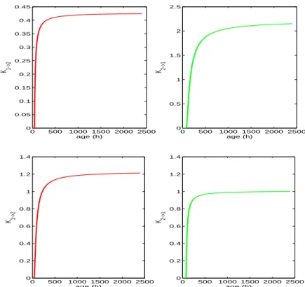
3.2. Internal validation. To make sure that our numerical results were in agreement with the biological data that we used to build our model (“internal validation”), we performed simulations in the case of no time control, that is,Ki→i+1(x, t) = Ki→i+1(x) (i = 1, 2), where theKi→i+1(x) were given by the expression (10). As we only wanted, in this inter-nal validation stage, to compare with biological data numerical results that were performed on the basis of modelling assumptions that corresponded to the two experimental condi-tions (10% and 15% of FBS), without assessing velocities, we assumed here that velocities v1andv2were constant, both equal to 1.
The graphs of the transition rates we obtained from formula (10) and experimental data are presented on Figure4.
0 500 1000 1500 2000 2500 0 0.05 0.1 0.15 0.2 0.25 0.3 0.35 0.4 0.45 age (h) K 1−>2 0 500 1000 1500 2000 2500 0 0.5 1 1.5 2 2.5 age (h) K 2−>1 0 500 1000 1500 2000 2500 0 0.2 0.4 0.6 0.8 1 1.2 1.4 age (h) K 1−>2 0 500 1000 1500 2000 2500 0 0.2 0.4 0.6 0.8 1 1.2 1.4 age (h) K 2−>1
FIGURE 4. Transition rates from G1 to S/G2/M (left) and from
S/G2/M to G1 (right) for the two experimental conditions, i.e. 10%
FBS (top) and 15% FBS (bottom). These rates are functions of age of cells in the phases only.
Figure5presents the time evolution of the percentage of cells in phasesG1andS/G2/M over the duration of one cell cycle resulting from numerical and biological experiments (biological data were preliminarily synchronised “by hand”, i.e., by deciding that all cells were at age nought in phaseG1at the beginning of simulations). We notice that modelled numerical data are very close to the raw biological data in the two experimental condi-tions. Therefore, we can conclude that the model and the method used to represent the proliferation phenomenon and fit our experimental data may have led us close to biological likelihood.
As mentioned in Section2.1, the growth exponentλ, first eigenvalue of System (2), can be computed from Lotka’s equation (cf Equation (3) and [12] for details). In the particular case of our experimentally based study described above, we had:
µ 1 + λ β1 ¶α1µ 1 + λ β2 ¶α2 eλ(γ1+γ2)= 2 (12) With the coefficients of the two Gamma distributions identified from FUCCI data (see
Ta-ble2) wherev1 = v2 = 1, this yielded λ ≈ 0.033h−1for the experiment with a medium
composed of 10% of FBS and λ ≈ 0.038h−1for the experiment with a medium composed
0 5 10 15 20 25 30 35 0 0.1 0.2 0.3 0.4 0.5 0.6 0.7 0.8 0.9 1 time (h) % of cells in G1 and SG2M G1 sim SG2M sim G1 data SG2M data
FIGURE5. Time evolution of the percentages of cells inG1(red or deep
grey) andS/G2/M (green or light grey) phases from biological data
(dashed line) and from numerical simulations (solid line), in the case of 10% FBS (top) and 15% FBS (bottom). Our model results in a good approximation of the biological data.
Td= 20.8h and Td = 18.1h. These figures are summarised in Table4.
10% FBS 15% FBS λ 0.033h−1 0.038h−1 Td 20.8h 18.1h
TABLE 4. Computed growth exponent (λ) and corresponding doubling time (Td) of the cell population for two experimental conditions (culture
medium composed of 10% of FBS or of 15% of FBS).
3.3. Simulations. We performed model simulations by means of the parameters identified
time evolution of the percentages of cells inG1and inS/G2/M and of the total population are presented on Figure6.
As expected, the oscillations of the percentages of cells inG1 and inS/G2/M were
damped. These percentages rapidly reached a steady state. This phenomenon reflects the progressive desynchronisation of cells in the population (asynchronous cell growth [1,2,
3]). We could notice that, even if the cell population submitted to 15% of FBS grew faster than the one submitted to 10% of FBS, desynchronisation occurred more rapidly in the case of 10% of FBS than in the case of 15% of FBS, i.e., it took longer for cells to desynchronise in the culture medium composed of 15% of FBS than in the medium composed of 10% of FBS. This corresponds to a lower phase duration variability in the case of 15% of FBS than in the case of 10% of FBS, lower variability in phase duration meaning sharper phase transition (cf. Section2.2.3).
As remarked in Section2.2.3and in Table4, an increased concentration in FBS (hence
in growth factors) in the medium resulted in shorter durations of phasesG1andS/G2/M
and thus in faster cell proliferation.
0 100 200 300 400 0 0.2 0.4 0.6 0.8 1 time (h) % of cells in G1 and SG2M G1 SG2M 0 100 200 300 400 0 2 4 6 8 10 12x 10 4 time (h)
total density of cells
0 100 200 300 400 0 0.2 0.4 0.6 0.8 1 time (h) % of cells in G1 and SG2M G1 SG2M 0 100 200 300 400 0 1 2 3 4 5 6 7x 10 5 time (h)
total density of cells
FIGURE 6. Time evolution of the percentages of cells inG1 (left, red
or deep grey) andS/G2/M (left, green or light grey) phases and of the
total population (right), in the case of 10% of FBS (top) and 15% of FBS (bottom). Cell desynchronisation occurs less rapidly and the population grows faster (λ ≈ 0.038h−1 vs. λ ≈ 0.033h−1) in the case of 15% of
FBS than in the case of 10% of FBS.
To model the effects of higher growth factor concentration in the medium on cell pop-ulation dynamics, we considered the experimental data for a concentration of 10% of FBS in the medium as reference data. Our aim was to recover the population dynamics for a concentration of 15% of FBS in the medium using this reference population as a basis. We
assumed that FBS influenced only cell ageing velocity and we wanted to check how this assumption was consistent with our biological data.
We thus calculated the probability density function deduced from the distribution of the
durations of phasesG1 andS/G2/M fitted in the population of cells proliferating in a
medium composed of 10% of FBS, using a shifted Gamma distribution model, whose
pa-rameters were found to beα1 = 1.80, β1 = 0.43h−1, γ1 = 4.83h, α2 = 16.96, β2 =
2.22h−1, γ2= 4.37h. From these figures we deduced the transition rates K
i→i+1,10%
un-der the assumptionv1= v2= 1 (cf Section2.2.3) and subsequently used these parameters of the age-structured model, except thatv1andv2 were no longer fixed, to identify these velocities in the case of 15% of FBS in the medium.
For convenience in this preliminary study, we assumed that v1 = v2 = v, i.e., that
15% FBS cells were ageing with the same, constant, velocity in G1 and in S/G2/M .
This velocityv was then viewed as a parameter to fit the percentages of cells in G1and S/G2/M resulting from the biological experiment with a medium composed of 15% of FBS (and synchronised “by hand” as in Section3.2). Thus the model we used was:
∂ ∂tni(t, x) + v ∂
∂xni(t, x) + Ki→i+1,10%(x) ni(t, x) = 0 i = 1, 2 ,
n2(t, x = 0) = Z ξ≥0 K1→2,10%(ξ) n1(t, ξ) dξ , n1(t, x = 0) = 2 Z ξ≥0 K2→1,10%(ξ) n2(t, ξ) dξ , (13)
whereKi→i+1,10%corresponded to the transition rates determined in the case of 10% FBS (cf Section2.2.3).
Our aim was thus to minimise the mean squared error that quantified the discrepancy
between the percentages of cells inG1and inS/G2/M computed by Equations (13) and
the experimental ones. We thus used the mean squared method by means of the fmincon Matlab function with the velocityv as parameter (the constraint being the positivity of v).
This method led to a computed value ofv equal to 1.095. The corresponding computed
and experimental percentages of cells inG1andS/G2/M are presented on Figure7. We
can notice that modelled numerical data were very close to raw biological data.
This valuev = 1.095 led to an exponential growth exponent λ (computed by means of
Equation (3)) equal to 0.045h−1and so to a doubling timeTdequal to 15.4h. These fig-ures tend to demonstrate that cells would proliferate approximately 10% faster in a medium composed of 15% of FBS than in a medium composed of 10% of FBS.
4. Conclusion and discussion. Growth factors, such as those contained in foetal bovine serum (FBS) are known to influence cell cycle dynamics. A lot of studies were and are still performed by scientists aiming at fully understanding the underlying mechanisms, see for instance [14,16,25,29,30,31,45]. We proposed an age-structured mathematical model whose parameters were computed on the basis of biological data, and that enabled us to analyse the cell synchronisation in the cell cycle according to the FBS concentration. This model also enabled us to recover the effects of an increase in the FBS concentration in the culture medium.
In our biological data, FBS decreased both the durations ofG1 andS/G2/M . These
results are in agreement with the results presented in the literature, for instance in [16,31]. In [16], the authors studied the effects of several concentrations of epidermal growth factor
FIGURE7. Time evolution of the percentages of cells inG1(red or deep
grey) andS/G2/M (green or light grey) phases from biological data in
the case of 15% FBS (dashed line) and from numerical simulations (solid line) resulting from Equations (13) forv = 1.095. Our model results in a good approximation of the biological data.
(EGF) on the proliferation and cell cycle regulation of cultured human amnion epithelial cells, using flow cytometry and gene expression measurements. They concluded that EGF increase resulted in reduced expression of the cell cycle control genes, which explained the
increased concentration of cells inS and G2/M phases they observed when using EGF
supplementation.
The value of the predicted exponential growth exponentλ for the case of 15% FBS (λ = 0.045h−1) was higher than the one we computed on the basis of the raw experimental data (λ = 0.038h−1). Nevertheless it seemed to us that the experimental data were “visually” better fitted by the predictive model (Equations (13)) than by the experimentally-based model (Equations (1)). This difference could be due to the fact that we directly fitted results of the model (percentages of cell inG1andS/G2/M ) instead of fitting it indirectly, i.e., through the Gamma distributions. Another way to improve the predictive character of our model would be to recur to another minimisation method (e.g., CMAES [22]).
Moreover, in this preliminary study, we assumed that FBS only impacted the cell ageing
velocities, in the same manner in the phase G1 as in the phase S/G2/M . In fact, the
mechanisms leading to changes in the cell cycle dynamics due to an increase (or decrease) of the FBS concentration in the culture medium might be much more complex.
Indeed, one may naturally question the way in which we investigated the effect of an increase in growth factors on the cell cycle model parameters: we focused on the velocity
parametersv1andv2with which phasesG1andS/G2/M are cruised by proliferating cell
populations in the division cycle, which implicitly assumes that protein synthesis
mech-anisms in phasesG1andG2, the major biological phenomena occurring in these phases,
are the main targets of growth factors, and this may be an oversimplified modelling as-sumption. Indeed, as mentioned in the introduction, it is known that growth factors affect in particular Cyclin D and its inhibitors at the restriction point of phaseG1, which could be differently represented in the model, namely by a direct action on phase transition rates Ki→i+1. This has been done only graphically (Figure4) in this paper, where the choice made here was to focus on velocity parametersv1andv2.
We based our study on two FBS concentrations. Biological FUCCI data performed on other cell types (healthy and/or cancer cells) with other varying FBS concentrations in the culture medium would help us to further analyse the effects of FBS on the cell cycle dy-namics and thus to improve the model predictability.
In a forthcoming work, we plan to introduce time control in the model presented in this paper in order to analyse the effect of increasing the FBS concentration of the cul-ture medium on cell circadian clocks. Such an analysis could help us to better understand the role of the circadian clock in cell cycle regulation of healthy and cancer cells in the presence of growth factor receptor (GFR) inhibitors. This should prove helpful to design theoretically optimised cancer treatments, that combine cytotoxic drugs, that exert their main action by arresting the cell cycle at phase transitions via DNA damage, ATM trigger-ing and p53 control, and GFR blockers. Such therapeutic combinations, currently in use in the clinic ([34], see also [9] and references therein), should indeed benefit from better knowledge of interactions between growth factors and the cell cycle from a modelling point of view.
Acknowledgments. This work has been supported by a grant from the European Research Area in Systems Biology (ERASysBio+) to the French National Research Agency (ANR) #ANR-09-SYSB-002 for the research network Circadian and Cell Cycle Clock Systems in Cancer (C5Sys) coordinated by Francis L´evi (INSERM U776, Villejuif, France) and by the University of Nice Sophia-Antipolis, CNRS and INSERM.
The authors heartily thank T. Lepoutre (Inria Grenoble - Rhˆone-Alpes, France) for fruit-ful discussions.
REFERENCES
[1] O. Arino. A survey of structured cell population dynamics. Acta Biotheor, 43(1-2):3–25, 1995.
[2] O. Arino and M. Kimmel. Comparison of approaches to modeling of cell population dynamics. SIAM J. Appl. Math., 53:1480–1504, 1993.
[3] O. Arino and E. Sanchez. A survey of cell population dynamics. J. Theor. Med., 1:35–51, 1997.
[4] D. Barbolosi, A. Benabdallah, F. Hubert, and F. Verga. Mathematical and numerical analysis for a model of growing metastatic tumors. Math Biosci, 218(1):1–14, 2009.
[5] B. Basse, B. C. Baguley, E. S. Marshall, G. C. Wake, and D. J. N. Wall. Modelling the flow [corrected] cytometric data obtained from unperturbed human tumour cell lines: parameter fitting and comparison. Bull Math Biol, 67(4):815–830, 2005.
[6] B. Basse and P. Ubezio. A generalised age- and phase-structured model of human tumour cell populations both unperturbed and exposed to a range of cancer therapies. Bull Math Biol, 69(5):1673–1690, 2007.
[7] S. Benzekry, N. Andr´e, A. Benabdallah, J. Ciccolini, C. Faivre, F. Hubert, and D. Barbolosi. Modeling the impact of anticancer agents on metastatic spreading. Mathematical Modelling of Natural Phenomena, 7(1):306–336, 2012.
[8] F. Billy, J. Clairambault, O. Fercoq, S. Gaubert, T. Lepoutre, T. Ouillon, and S. Saito. Synchronisation and control of proliferation in cycling cell population models with age structure. Math. Comp. Simul., 2012. in press, available on line Apr. 2012.
[9] J. Clairambault. Optimizing cancer pharmacotherapeutics using mathematical modeling and a systems biol-ogy approach. Personalized Medicine, 8:271–286, 2011.
[10] J. Clairambault, S. Gaubert, and T. Lepoutre. Comparison of Perron and Floquet eigenvalues in age struc-tured cell division models. Mathematical Modelling of Natural Phenomena, 4:183–209, 2009.
[11] J. Clairambault, S. Gaubert, and T. Lepoutre. Circadian rhythm and cell population growth. Mathematical and Computer Modelling, 53:1558–1567, 2011.
[12] J. Clairambault, B. Laroche, S. Mischler, and B. Perthame. A mathematical model of the cell cycle and its control. Technical report, Number 4892, INRIA, Domaine de Voluceau, BP 105, 78153 Rocquencourt, France, 2003.
[13] A. A. Cohen, T. Kalisky, A. Mayo, N. Geva-Zatorsky, T. Danon, I. Issaeva, R. Kopito, N. Perzov, R. Milo, A. Sigal, and U. Alon. Protein dynamics in individual human cells: Experiment and theory. PLoS one, 4:1–12, 2009.
[14] M. Cross and T. M. Dexter. Growth factors in development, transformation, and tumorigenesis. Cell, 64(2):271–280, Jan 1991.
[15] S. Davis and D. K. Mirick. Circadian disruption, shift work and the risk of cancer: a summary of the evidence and studies in seattle. Cancer Causes Control, 17(4):539–545, 2006.
[16] S. S. Fatimah, G. C. Tan, K. H. Chua, A. E. Tan, and A. R. Hayati. Effects of epidermal growth factor on the proliferation and cell cycle regulation of cultured human amnion epithelial cells. J Biosci Bioeng, 114(2):220–227, 2012.
[17] E. Filipski, X. M. Li, and F. L´evi. Disruption of circadian coordination and malignant growth. Cancer Causes Control, 17(4):509–514, 2006.
[18] E. Filipski, P. Subramanian, J. Carri`ere, C. Guettier, H. Barbason, and F. L´evi. Circadian disruption acceler-ates liver carcinogenesis in mice. Mutat Res, 680(1-2):95–105, 2009.
[19] D. A. Foster, P. Yellen, L. Xu, and M. Saqcena. Regulation of g1 cell cycle progression: Distinguishing the restriction point from a nutrient-sensing cell growth checkpoint(s). Genes Cancer, 1(11):1124–1131, Nov 2010.
[20] M. Gyllenberg and G. F. Webb. A nonlinear structured population model of tumor growth with quiescence. J Math Biol, 28(6):671–694, 1990.
[21] J. Hansen. Risk of breast cancer after night- and shift work: current evidence and ongoing studies in den-mark. Cancer Causes Control, 17(4):531–537, 2006.
[22] N. Hansen. The CMA evolution strategy: a comparing review. towards a new evolutionary computation. In J. Lozano, P. Larranaga, I. Inza, and E. Bengoetxea, editors, Advances on Estimation of Distribution Algorithms, pages 75–102. Springer, New York, 2006.
[23] P. Hinow, S. E. Wang, C. L. Arteaga, and G. F. Webb. A mathematical model separates quantitatively the cytostatic and cytotoxic effects of a HER2 tyrosine kinase inhibitor. Theor Biol Med Model, 4:14, 2007.
[24] K. Iwata, K. Kawasaki, and N. Shigesada. A dynamical model for the growth and size distribution of multiple metastatic tumors. J Theor Biol, 203(2):177–186, 2000.
[25] S. M. Jones and A. Kazlauskas. Connecting signaling and cell cycle progression in growth factor-stimulated cells. Oncogene, 19(49):5558–5567, Nov 2000.
[26] Y. Kheifetz, Y. Kogan, and Z. Agur. Long-range predictability in models of cell populations subjected to phase-specific drugs: growth-rate approximation using properties of positive compact operators. Math. Mod-els Methods Appl. Sci., 16(7, suppl.):1155–1172, 2006.
[27] F. L´evi, A. Okyar, S. Dulong, P. F. Innominato, and J. Clairambault. Circadian timing in cancer treatments. Annu Rev Pharmacol Toxicol, 50:377–421, 2010.
[28] F. L´evi and U. Schibler. Circadian rhythms: mechanisms and therapeutic implications. Annu Rev Pharmacol Toxicol, 47:593–628, 2007.
[29] J. Massagu´e. How cells read TGF-β signals. Nat Rev Mol Cell Biol, 1(3):169–178, Dec 2000.
[30] J. Massagu´e, S. W. Blain, and R. S. Lo. TGFβ signaling in growth control, cancer, and heritable disorders. Cell, 103(2):295–309, Oct 2000.
[31] A. L. Mazlyzam, B. S. Aminuddin, L. Saim, and B. H. I. Ruszymah. Human serum is an advantageous supplement for human dermal fibroblast expansion: clinical implications for tissue engineering of skin. Arch Med Res, 39(8):743–752, 2008.
[32] H. H. McAdams and A. Arkin. Stochastic mechanisms in gene expression. Proc. Natl. Acad. Sci. USA, 31:814–819, 1997.
[33] A. McKendrick. Applications of mathematics to medical problems. Proc. Edinburgh Math. Soc., 54:98–130, 1926.
[34] J. Mendelsohn and J. Baselga. Status of epidermal growth factor receptor antagonists in the biology and treatment of cancer. J. Clin. Oncol., 14:2787–2799, 2003.
[35] J. Metz and O. Diekmann. The dynamics of physiologically structured populations, volume 68 of Lecture notes in biomathematics. Springer, New York, 1986.
[36] A. B. Pardee. A restriction point for control of normal animal cell proliferation. Proc Natl Acad Sci U S A, 71(4):1286–1290, 1974.
[37] B. Perthame. Transport Equations in Biology. Frontiers in Mathematics series. Birkh¨auser, Boston, 2007.
[38] S. I. Reed, E. Bailly, V. Dulic, L. Hengst, D. Resnitzky, and J. Slingerland. G1 control in mammalian cells. J Cell Sci Suppl, 18:69–73, 1994.
[39] D. Resnitzky, M. Gossen, H. Bujard, and S. I. Reed. Acceleration of the G1/S phase transition by expression of cyclins D1 and E with an inducible system. Mol Cell Biol, 14(3):1669–1679, 1994.
[40] B. Ribba, O. Saut, T. Colin, D. Bresch, E. Grenier, and J. P. Boissel. A multiscale mathematical model of avascular tumor growth to investigate the therapeutic benefit of anti-invasive agents. J Theor Biol, 243(4):532–541, 2006.
[41] A. Sakaue-Sawano, H. Kurokawa, T. Morimura, A. Hanyu, H. Hama, H. Osawa, S. Kashiwagi, K. Fukami, T. Miyata, H. Miyoshi, T. Imamura, M. Ogawa, H. Masai, and A. Miyawaki. Visualizing spatiotemporal dynamics of multicellular cell-cycle progression. Cell, 132(3):487–498, 2008.
[42] A. Sakaue-Sawano, K. Ohtawa, H. Hama, M. Kawano, M. Ogawa, and A. Miyawaki. Tracing the silhouette of individual cells in S/G2/M phases with fluorescence. Chem Biol, 15(12):1243–1248, 2008.
[43] V. Shahreazaei and P. G. Swain. Analytical distributions for stochastic gene expression. Proc. Natl. Acad. Sci. USA, 105:17256–17261, 2008.
[44] E. Sherer, E. Tocce, R. E. Hannemann, A. E. Rundell, and D. Ramkrishna. Identification of age-structured models: cell cycle phase transitions. Biotechnol Bioeng, 99(4):960–974, 2008.
[45] R. Taub. Liver regeneration: from myth to mechanism. Nat Rev Mol Cell Biol, 5(10):836–847, Oct 2004.
[46] G. Webb. Resonance phenomena in cell population chemotherapy models. Rocky Mountain J. Math, 20(4):1195–1216, 1990.
[47] A. Zetterberg, O. Larsson, and K. G. Wiman. What is the restriction point? Curr Opin Cell Biol, 7(6):835– 842, Dec 1995.
Received August 06, 2012; Accepted xx xx, 201x.
E-mail address: [email protected] E-mail address: [email protected] E-mail address: [email protected] E-mail address: [email protected] E-mail address: [email protected]