B
TUTORIAL
Microsoft Access Tutorial
Microsoft Access is a relational database package that runs on the Microsoft Windows operating system. This tutorial was pre-pared using Access 2003.
Before using this tutorial, you should know the fundamentals of Microsoft Access and know how to use Windows. This tutorial teaches you some advanced Access skills you’ll need to do data-base case studies. This tutorial concludes with a discussion of com-mon Access problems and how to solve them.
A preliminary caution: Always observe proper file-saving and closing procedures. Use these steps to exit from Access: (1) File— Close, then (2) File—Exit. This gets you back to Windows. Always end your work with these two steps. Never pull out your disk, CD, or other portable storage device and walk away with work remaining on the screen, or you will lose your work.
To begin this tutorial, you will create a new database called
Employee. AT THE KEYBOARD
Open a new database (in the Task Pane—New—Blank database). (According to Microsoft, the Task Pane is a universal remote con-trol, which saves the user steps.) Call the database Employee. If you are saving to a floppy disk, first select the drive (A:), and then enter the filename. EMPLOYEE.mdb would be a good choice. Your opening screen should resemble the screen shown in Figure B-1.
In this tutorial, the screen shown in Figure B-1 is called the Database window. From this screen, you can create or change objects.
C
REATINGT
ABLESYour database will contain data about employees, their wage rates, and their hours worked.
Defining Tables
In the Database window, make three new tables, using the instructions that follow.
AT THE KEYBOARD
(1) Define a table called EMPLOYEE.
This table contains permanent data about employees. To create it, in the Table Objects screen, click New, then Design View, and then define the table EMPLOYEE. The table’s fields are Last Name, First Name, SSN (Social Security Number), Street Address, City, State, Zip, Date Hired, and US Citizen. The field SSN is the primary key field. Change the length of text fields from the default 50 spaces to more appropriate lengths; for example, the field Last Name might be 30 spaces, and the Zip field might be 10 spaces. Your completed definition should resemble the one shown in Figure B-2.
Figure B-2 Fields in the EMPLOYEE table
When you’re finished, choose File—Save. Enter the name desired for the table (here, EMPLOYEE). Make sure that you specify the name of the table, not the database itself. (Here, it is a coincidence that the EMPLOYEE table has the same name as its database file.) (2) Define a table called WAGE DATA.
This table contains permanent data about employees and their wage rates. The table’s fields are SSN, Wage Rate, and Salaried. The field SSN is the primary key field. Use the data types shown in Figure B-3. Your definition should resemble the one shown in Figure B-3.
Figure B-3 Fields in the WAGE DATA table
T
utorial B
T
utorial B
(3) Define a table called HOURS WORKED.
The purpose of this table is to record the number of hours employees work each week in the year. The table’s fields are SSN (text), Week # (number—long integer), and Hours (number— double). The SSN and Week# are the compound keys.
In the following example, the employee having SSN 089-65-9000 worked 40 hours in Week 1 of the year and 52 hours in Week 2.
SSN Week # Hours
089-65-9000 1 40
089-65-9000 2 52
Note that no single field can be the primary key field. Why? Notice that 089-65-9000 is an entry for each week. If the employee works each week of the year, at the end of the year, there will be 52 records with that value. Thus, SSN values will not distinguish records. However, no other single field can distinguish these records either, because other employees will have worked during the same week number, and some employees will have worked the same number of hours (40 would be common).
However, a table must have a primary key field. What is the solution? Use a com-pound primary key; that is, use values from more than one field. Here, the comcom-pound key to use consists of the field SSN plus the Week # field. Why? There is only one combina-tion of SSN 089-65-9000 and Week# 1—those values can occur in only one record; there-fore, the combination distinguishes that record from all others.
How do you set a compound key? The first step is to highlight the fields in the key. These must appear one after the other in the table definition screen. (Plan ahead for this format.) Alternately, you can highlight one field, hold down the Control key, and highlight the next field.
AT THE KEYBOARD
For the HOURS WORKED table, click in the first field’s left prefix area, hold down the but-ton, then drag down to highlight names of all fields in the compound primary key. Your screen should resemble the one shown in Figure B-4.
Figure B-4 Selecting fields as the compound primary key for the HOURS WORKED table
Now, click the Key icon. Your screen should resemble the one shown in Figure B-5.
Figure B-5 The compound primary key for the HOURS WORKED table
That completes the compound primary key and the table definition. Use File—Save to save the table as HOURS WORKED.
Adding Records to a Table
At this point, all you have done is to set up the skeletons of three tables. The tables have no data records yet. If you were to print the tables, all you would see would be column headings (the field names). The most direct way to enter data into a table is to select the table, open it, and type the data directly into the cells.
AT THE KEYBOARD
At the Database window, select Tables, then EMPLOYEE. Then select Open. Your data-entry screen should resemble the one shown in Figure B-6.
Figure B-6 The data-entry screen for the EMPLOYEE table
The table has many fields, and some of them may be off the screen, to the right. Scroll to see obscured fields. (Scrolling happens automatically as data is entered.) Figure B-6 has been adjusted to view all fields on one screen.
Type in your data, one field value at a time. Note that the first row is empty when you begin. Each time you finish a value, hit Enter, and the cursor will move to the next cell. After the last cell in a row, the cursor moves to the first cell of the next row, and Access automati-cally saves the record. (Thus, there is no File—Save step after entering data into a table.) Dates (for example, Date Hired) are entered as “6/15/04” (without the quotation marks). Access automatically expands the entry to the proper format in output.
Yes/No variables are clicked (checked) for Yes; otherwise (for No), the box is left blank. You can click the box from Yes to No, as if you were using a toggle switch.
If you make errors in data entry, click in the cell, backspace over the error, and type the correction.
Enter the data shown in Figure B-7 into the EMPLOYEE table.
Figure B-7 Data for the EMPLOYEE table
Note that the sixth record is your data record. The edit pencil in the left prefix area marks that record. Assume that you live in Newark, Minnesota, were hired on today’s date (enter the date), and are a U.S. citizen. (Later in this tutorial, you will see that one entry is for the author’s name and the SSN 099-11-3344 for this record.)
T
utorial B
T
utorial B
Figure B-8 Data for the WAGE DATA table
Again, you must enter your SSN. Assume that you earn $8 an hour and are not salaried. (Note that Salaried = No implies someone is paid by the hour. Those who are salaried do not get paid by the hour, so their hourly rate is shown as 0.00.)
Open the HOURS WORKED table and enter the data shown in Figure B-9 into the table.
Figure B-9 Data for the HOURS WORKED table
Notice that salaried employees are always given 40 hours. Non-salaried employees (including you) might work any number of hours. For your record, enter your SSN, 60 hours worked for Week 1, and 55 hours worked for Week 2.
C
REATINGQ
UERIESBecause you can already create basic queries, this section teaches you the kinds of advanced queries you will create in the Case Studies.
Using Calculated Fields in Queries
A calculated field is an output field that is made from other field values. A calculated field is not a field in a table; it is created in the query generator. The calculated field does not become part of the table—it is just part of query output. The best way to explain this process is by working through an example.
AT THE KEYBOARD
Suppose that you want to see the SSNs and wage rates of hourly workers, and you want to see what the wage rates would be if all employees were given a 10% raise. To do this,
show the SSN, the current wage rate, and the higher rate (which should be titled New Rate in the output). Figure B-10 shows how to set up the query.
Figure B-10 Query set-up for the calculated field
The Salaried field is needed, with the Criteria =No, to select hourly workers. The Show box for that field is not checked, so the Salaried field values will not show in the query output. Note the expression for the calculated field, which you see in the rightmost field cell:
New Rate: 1.1*[Wage Rate]
New Rate: merely specifies the desired output heading. (Don’t forget the colon.) The 1.1*[Wage Rate] multiplies the old wage rate by 110%, which results in the 10% raise.
In the expression, the field name Wage Rate must be enclosed in square brackets. This is a rule: Any time that an Access expression refers to a field name, it must be enclosed in square brackets.
If you run this query, your output should resemble that shown in Figure B-11.
Figure B-11 Output for a query with calculated field
Notice that the calculated field output is not shown in Currency format; it’s shown as a Double—a number with digits after the decimal point. To convert the output to Currency for-mat, click the line above the calculated field expression, thus activating the column (it dark-ens). Your data-entry screen should resemble the one shown in Figure B-12.
T
utorial B
T
utorial B
Figure B-12 Activating a calculated field in query design
Then select View—Properties. Click the Format drop-down menu. A window, such as the one shown in Figure B-13, will pop up.
Figure B-13 Field Properties of a calculated field
Click Currency. Then click the upper-right X to close the window. Now when you run the query, the output should resemble that shown in Figure B-14.
Figure B-14 Query output with formatted calculated field
Next, let’s look at how to avoid errors when making calculated fields.
Avoiding Errors in Making Calculated Fields
Follow these guidelines to avoid making errors in calculated fields:
• Don’t put the expression in the Criteria cell, as if the field definition were a filter. You are making a field, so put the expression in the Field cell.
• Spell, capitalize, and space a field’s name exactly as you did in the table definition. If the table definition differs from what you type, Access thinks you’re defining a new field by that name. Access then prompts you to enter values for the new field, which it calls a “Parameter Query” field. This is easy to debug because of the tag Parameter Query. If Access asks you to enter values for a Parameter, you almost certainly have misspelled a field name in an expression in a calculated field or a criterion.
Example: Here are some errors you might make for Wage Rate: Misspelling: (Wag Rate)
Case change: (wage Rate / WAGE RATE) Spacing change: (WageRate / Wage Rate)
• Don’t use parentheses or curly braces instead of the square brackets. Also, don’t put parentheses inside square brackets. You are allowed to use parentheses outside the square brackets, in the normal algebraic manner.
Example: Suppose that you want to multiply Hours times Wage Rate, to get a field called Wages Owed. This is the correct expression:
Wages Owed: [Wage Rate]*[Hours] This would also be correct:
Wages Owed: ([Wage Rate]*[Hours])
But it would not be correct to leave out the inside brackets, which is a common error: Wages Owed: [Wage Rate*Hours]
“Relating” Two (or More) Tables by the Join Operation
Often, the data you need for a query is in more than one table. To complete the query, you must join the tables. One rule of thumb is that joins are made on fields that have common values, and those fields can often be key fields. The names of the join fields are irrelevant— the names may be the same, but that is not a requirement for an effective join.
Make a join by first bringing in (Adding) the tables needed. Next, decide which fields you will join. Then, click one field name and hold down the left mouse button while dragging the cursor over to the other field’s name in its window. Release the button. Access puts in a line, signifying the join. (Note: If there are two fields in the tables with the same name, Access will put in the line automatically, so you do not have to do the click-and-drag opera-tion.)
You can join more than two tables together. The common fields need not be the same in all tables; that is, you can “daisy-chain” them together.
A common join error is to Add a table to the query and then fail to link it to another table. You have a table just “floating” in the top part of the QBE screen! When you run the query, your output will show the same records over and over. This error is unmistakable because there is so much redundant output. The rules are: (1) add only the tables you need and (2) link all tables.
Next, you’ll work through an example of a query needing a join.
AT THE KEYBOARD
Suppose that you want to see the last names, SSNs, wage rates, salary status, and citizenship only for U.S. citizens and hourly workers. The data is spread across two tables, EMPLOYEE and WAGE DATA, so both tables are added, and five fields are pulled down. Criteria are then added. Set up your work to resemble that shown in Figure B-15.
T
utorial B
T
utorial B
Figure B-15 A query based on two joined tables
In Figure B-15, the join is on the SSN field. A field by that name is in both tables, so Access automatically puts in the join. If one field had been spelled SSN and the other Social Security Number, you would still join on these fields (because of the common values). You would click and drag to do this operation.
Now run the query. The output should resemble that shown in Figure B-16, with the exception of the name Brady.
Figure B-16 Output of a query based on two joined tables
Here is a quick review of Criteria: If you want data for employees who are U.S. citizens and who are hourly workers, the Criteria expressions go into the same Criteria row. If you want data for employees who are U.S. citizens or who are hourly workers, one of the expres-sions goes into the second Criteria row (the one that has the “or:” notation).
There is no need to print the query output or to save it. Go back to the Design View and close the query. Another practice query follows.
AT THE KEYBOARD
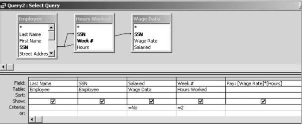
Suppose that you want to see the wages owed to hourly employees for Week 2. Show the last name, the SSN, the salaried status, the week #, and the wages owed. Wages will have to be a calculated field ([Wage Rate]*[Hours]). The criteria are =No for Salaried and =2 for the Week # (another “And” query). You’d set up the query the way it is displayed in Figure B-17.
Figure B-17 Query set-up for wages owed to hourly employees for Week 2
In the previous table, the calculated field column was widened so you can see the whole expression. To widen a column, remember to click the column boundary line and drag to the right.
Run the query. The output should be similar to that shown in Figure B-18 (if you format-ted your calculaformat-ted field to currency).
Figure B-18 Query output for wages owed to hourly employees for Week 2
Notice that it was not necessary to pull down the Wage Rate and Hours fields to make this query work. Return to the Design View. There is no need to save. Select File—Close.
Summarizing Data from Multiple Records (Sigma Queries)
You may want data that summarizes values from a field for several records (or possibly all records) in a table. For example, you might want to know the average hours worked for all employees in a week, or perhaps the total (sum of) all the hours worked. Furthermore, you might want data grouped (“stratified”) in some way. For example, you might want to know the average hours worked, grouped by all U.S. citizens versus all non-U.S. citizens. Access calls this kind of query a “summary” query, or a Sigma query. Unfortunately, this terminol-ogy is not intuitive, but the statistical operations that are allowed will be familiar. These oper-ations include the following:
Sum The total of some field’s values
Count A count of the number of instances in a field, that is, the number of records. Here, to get the number of employees, you’d count the number of SSN numbers.
T
utorial B
T
utorial B
Min The minimum of some field’s values Var The variance of some field’s values
StDev The standard deviation of some field’s values
AT THE KEYBOARD
Suppose that you want to know how many employees are represented in a database. The first step is to bring the EMPLOYEE table into the QBE screen. Do that now. The query will Count the number of SSNs, which is a Sigma query operation. Thus, you must bring down the SSN field.
To tell Access you want a Sigma query, click the little “Sigma” icon in the menu, as shown in Figure B-19.
Figure B-19 Sigma icon
This opens up a new row in the lower part of the QBE screen, called the Total row. At this point, the screen would resemble that shown in Figure B-20.
Figure B-20 Sigma query set-up
Note that the Total cell contains the words “Group By.” Until you specify a statistical operation, Access just assumes that a field will be used for grouping (stratifying) data.
To count the number of SSNs, click next to Group By, revealing a little arrow. Click the arrow to reveal a drop-down menu, as shown in Figure B-21.
Figure B-21 Choices for statistical operation in a Sigma query
Select the Count operator. (With this menu, you may need to scroll to see the operator you want.) Your screen should now resemble that shown in Figure B-22.
Figure B-22 Count in a Sigma query
Run the query. Your output should resemble that shown in Figure B-23.
Figure B-23 Output of Count in a Sigma query
Notice that Access has made a pseudo-heading “CountOfSSN.” To do this, Access just spliced together the statistical operation (Count), the word Of, and the name of the field
T
utorial B
T
utorial B
(SSN). What if you wanted an English phrase, such as “Count of Employees,” as a heading? In the Design View, you’d change the query to resemble the one shown in Figure B-24.
Figure B-24 Heading change in a Sigma query
Now when you run the query, the output should resemble that shown in Figure B-25.
Figure B-25 Output of heading change in a Sigma query
There is no need to save this query. Go back to the Design View and Close.
AT THE KEYBOARD
Here is another example. Suppose that you want to know the average wage rate of employ-ees, grouped by whether they are salaried.
Figure B-26 shows how your query should be set up.
When you run the query, your output should resemble that shown in Figure B-27.
Figure B-27 Output of query for average wage rate of employees
Recall the convention that salaried workers are assigned zero dollars an hour. Suppose that you want to eliminate the output line for zero dollars an hour because only hourly-rate workers matter for this query. The query set-up is shown in Figure B-28.
Figure B-28 Query set-up for non-salaried workers only
When you run the query, you’ll get output for non-salaried employees only, as shown in Figure B-29.
Figure B-29 Query output for non-salaried workers only
Thus, it’s possible to use a Criteria in a Sigma query without any problem, just as you would with a “regular” query.
There is no need to save the query. Go back to the Design View and Close.
AT THE KEYBOARD
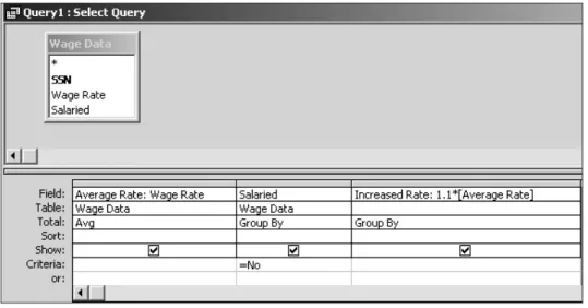
You can make a calculated field in a Sigma query. Assume that you want to see two things for hourly workers: (1) the average wage rate—call it Average Rate in the output; and (2) 110% of this average rate—call it the Increased Rate.
T
utorial B
T
utorial B
You already know how to do certain things for this query. The revised heading for the average rate will be Average Rate (Average Rate: Wage Rate, in the Field cell). You want the Average of that field. Grouping would be by the Salaried field (with Criteria: =No, for hourly workers).
The most difficult part of this query is to construct the expression for the calculated field. Conceptually, it is as follows:
Increased Rate: 1.1*[The current average, however that is denoted]
The question is how to represent [The current average]. You cannot use Wage Rate for this, because that heading denotes the wages before they are averaged. Surprisingly, it turns out that you can use the new heading (Average Rate) to denote the averaged amount. Thus:
Increased Rate: 1.1*[Average Rate]
Counterintuitively, you can treat “Average Rate” as if it were an actual field name. Note, however, that if you use a calculated field, such as Average Rate, in another calculated field, as shown in Figure B-30, you must show that original calculated field in the query output, or the query will ask you to “enter parameter value,” which is incorrect. Use the set-up shown in Figure B-30.
Figure B-30 Using a calculated field in another calculated field
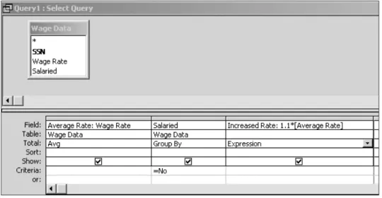
However, if you ran the query now shown in Figure B-30, you’d get some sort of error message. You do not want Group By in the calculated field’s Total cell. There is not a statistical operator that applies to the calculated field. You must change the Group By operator to Expression. You may have to scroll to get to Expression in the list. Figure B-31 shows how your screen should look.
Figure B-31 Changing the Group By to an Expression in a Sigma query
Figure B-32 shows how the screen looks before running the query.
Figure B-32 An Expression in a Sigma query
Figure B-33 shows the output of the query.
Figure B-33 Output of an Expression in a Sigma query
There is no need to save the query definition. Go back to the Design View. Select File—Close.
T
utorial B
T
utorial B
Using the Date() Function in Queries
Access has two date function features that you should know about. A description of them follows:
1. The following built-in function gives you today’s date: Date()
You can use this function in a query criteria or in a calculated field. The function “returns” the day on which the query is run—that is, it puts that value into the place where the function is in an expression.
2. Date arithmetic lets you subtract one date from another to obtain the number of days difference. Access would evaluate the following expression as the integer 5 (9 less 4 is 5).
10/9/2006 – 10/4/2006
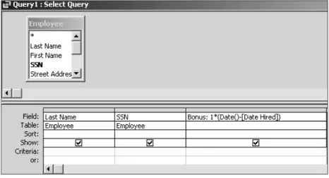
Here is an example of how date arithmetic works. Suppose that you want to give each employee a bonus equaling a dollar for each day the employee has worked for you. You’d need to calculate the number of days between the employee’s date of hire and the day that the query is run, then multiply that number by 1.
The number of elapsed days is shown by the following equation: Date() – [Date Hired]
Suppose that for each employee, you want to see the last name, SSN, and bonus amount. You’d set up the query as shown in Figure B-34.
Figure B-34 Date arithmetic in a query
Assume that you set the format of the Bonus field to Currency. The output will be similar to Figure B-35. (Your Bonus data will be different because you are working on a date differ-ent from the date when this tutorial was written.)
Figure B-35 Output of query with date arithmetic
Using Time Arithmetic in Queries
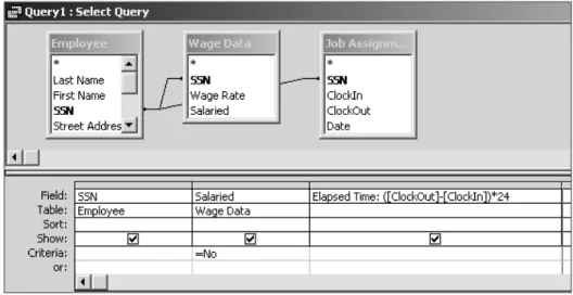
Access will also let you subtract the values of time fields to get an elapsed time. Assume that your database has a JOB ASSIGNMENTS table showing the times that non-salaried employ-ees were at work during a day. The definition is shown in Figure B-36.
Figure B-36 Date/Time data definition in the JOB ASSIGNMENTS table
Assume that the Date field is formatted for Long Date and that the ClockIn and ClockOut fields are formatted for Medium Time. Assume that, for a particular day, non-salaried workers were scheduled as shown in Figure B-37.
Figure B-37 Display of date and time in a table
You want a query that will show the elapsed time on premises for the day. When you add the tables, your screen may show the links differently. Click and drag the JOB ASSIGNMENTS, EMPLOYEE, and WAGE DATA table icons to look like those in Figure B-38.
T
utorial B
T
utorial B
Figure B-38 Query set-up for time arithmetic
Figure B-39 shows the output.
Figure B-39 Query output for time arithmetic
The output looks right. For example, employee 099-11-3344 was at work from 8:30 a.m. to 4:30 p.m., which is eight hours. But how does the odd expression that follows yield the correct answers?
([ClockOut] – [ClockIn]) * 24
Why wouldn’t the following expression, alone, work? [ClockOut] – [ClockIn]
This is the answer: In Access, subtracting one time from the other yields the decimal portion of a 24-hour day. Employee 099-11-3344 worked 8 hours, which is one-third of a day, so .3333 would result. That is why you must multiply by 24—to convert to an hour basis. Continuing with 099-11-3344, 1/3 x 24 = 8.
Note that parentheses are needed to force Access to do the subtraction first, before the multiplication. Without parentheses, multiplication takes precedence over subtraction. With the following expression, ClockIn would be multiplied by 24 and then that value would be subtracted from ClockOut, and the output would be a nonsense decimal number:
[ClockOut] – [ClockIn] * 24
Delete and Update Queries
Thus far, the queries presented in this tutorial have been Select queries. They select certain data from specific tables, based on a given criterion. You can also create queries to update the original data in a database. Businesses do this often, and in real time. For example, when you
order an item from a Web site, the company’s database is updated to reflect the purchase of the item by deleting it from inventory.
Let’s look at an example. Suppose that you want to give all the non-salaried workers a $.50 per hour pay raise. With the three non-salaried workers you have now, it would be easy simply to go into the table and change the Wage Rate data. But assume that you have 3,000 non-salaried employees. It would be much faster and more accurate to change each of the 3,000 non-salaried employees’ Wage Rate data by using an Update query to add the $.50 to each employee’s wage rate.
AT THE KEYBOARD
Let’s change each of the non-salaried employees’ pay via an Update query. Figure B-40 shows how to set up the query.
Figure B-40 Query set-up for an Update Query
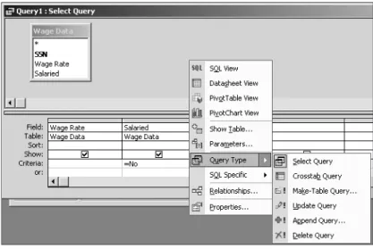
So far, this query is just a Select query. Place your cursor somewhere above the QBE grid, and then right-click the mouse. Once you are in that menu, choose Query Type— Update Query, as shown in Figure B-41.
T
utorial B
T
utorial B
Notice that you now have another line on the QBE grid called “Update to:”. This is where you specify the change or update to the data. Notice that you are going to update only the non-salaried workers by using a filter under the Salaried field. Update the Wage Rate data to Wage Rate plus $.50, as shown in Figure B-42. (Note the [ ] as in a calculated field.)
Figure B-42 Updating the wage rate for non-salaried workers
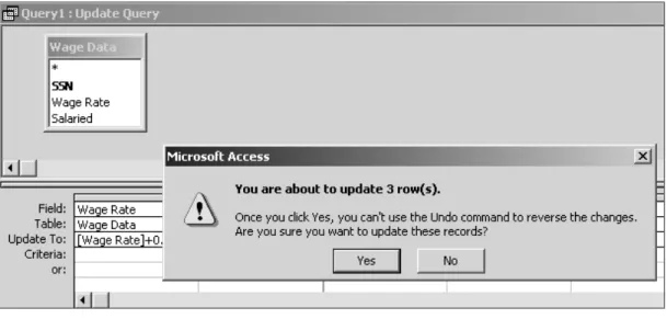
Now run the query. You will first get a warning message, as shown in Figure B-43.
Figure B-43 Update Query warning
Once you click “Yes,” the records will be updated. Check those updated records now by viewing the WAGE DATA table. Each salaried wage rate should now be increased by $.50. Note that in this example, you are simply adding $.50 to each salaried wage rate. You could add or subtract data from another table as well. If you do that, remember to call the field name in square brackets.
Delete queries work the same way as Update queries. Assume that your company has been taken over by the state of Delaware. The state has a policy of employing only Delaware residents. Thus, you must delete (or fire) all employees who are not only Delaware residents. To do this, you would first create a Select query using the EMPLOYEE table, right-click your mouse, choose Delete Query from Query Type, then bring down the State field and filter only
those records not in Delaware (DE). Do not perform this operation, but note that, if you did, the set-up would look like that in Figure B-44.
Figure B-44 Deleting all employees who are not Delaware residents
Parameter Queries
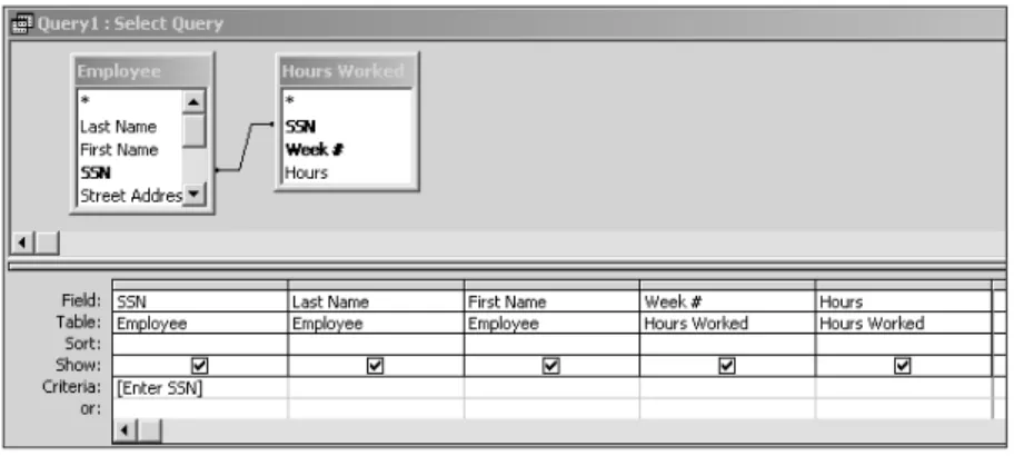
Another type of query, which is a type of Select query, is called a Parameter query. Here is an example: Suppose that your company has 5,000 employees. You might want to query the database to find the same kind of information again and again, only about different employ-ees. For example, you might want to query the database to find out how many hours a par-ticular employee has worked. To do this, you could run a query previously created and stored, but run it only for a particular employee.
AT THE KEYBOARD
Create a Select query with the format shown in Figure B-45.
Figure B-45 Design of a Parameter query begins as a Select query
T
utorial B
T
utorial B
Figure B-46 Design of a Parameter query
Note the square brackets, as you would expect to see in a calculated field.
Now run that query. You will be prompted for the specific employee’s SSN, as shown in Figure B-47.
Figure B-47 Enter Parameter Value dialog box
Type in your own SSN. Your query output should resemble that shown in Figure B-48.
Figure B-48 Output of a Parameter query
S
EVENP
RACTICEQ
UERIESThis portion of the tutorial is designed to provide you with additional practice in making queries. Before making these queries, you must create the specified tables and enter the records shown in the Creating Tables section of this tutorial. The output shown for the prac-tice queries is based on those inputs.
AT THE KEYBOARD
For each query that follows, you are given a problem statement and a “scratch area.” You are also shown what the query output should look like. Follow this procedure: Set up a query in Access. Run the query. When you are satisfied with the results, save the query and continue with the next query. You will be working with the EMPLOYEE, HOURS WORKED, and WAGE DATA tables.
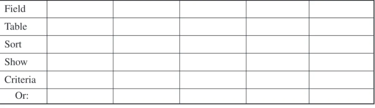
1. Create a query that shows the SSN, last name, state, and date hired for those living in Delaware and who were hired after 12/31/92. Sort (ascending) by SSN. (Sorting review: Click in the Sort cell of the field. Choose Ascending or Descending.) Use the table shown in Figure B-49 to work out your QBE grid on paper before creating your query.
Figure B-49 QBE grid template
Your output should resemble that shown in Figure B-50.
Figure B-50 Number 1 query output
2. Create a query that shows the last name, first name, date hired, and state for those living in Delaware or who were hired after 12/31/92. The primary sort (ascending) is on last name, and the secondary sort (ascending) is on first name. (Review: The Primary Sort field must be to the left of the Secondary Sort field in the query set-up.) Use the table shown in Figure B-51 to work out your QBE grid on paper before creat-ing your query.
Figure B-51 QBE grid template
If your name were Brady, your output would look like that shown in Figure B-52. Field Table Sort Show Criteria Or: Field Table Sort Show Criteria Or:
T
utorial B
T
utorial B
Figure B-52 Number 2 query output
3. Create a query that shows the sum of hours worked by U.S. citizens and by non-U.S. citizens (that is, group on citizenship). The heading for total hours worked should be Total Hours Worked. Use the table shown in Figure B-53 to work out your QBE grid on paper before creating your query.
Figure B-53 QBE grid template
Your output should resemble that shown in Figure B-54.
Figure B-54 Number 3 query output
4. Create a query that shows the wages owed to hourly workers for Week 1. The heading for the wages owed should be Total Owed. The output headings should be: Last Name, SSN, Week #, and Total Owed. Use the table shown in Figure B-55 to work out your QBE grid on paper before creating your query.
Field Table Total Sort Show Criteria Or:
Figure B-55 QBE grid template
If your name were Joseph Brady, your output would look like that in Figure B-56.
Figure B-56 Number 4 query output
5. Create a query that shows the last name, SSN, hours worked, and overtime amount owed for employees paid hourly who earned overtime during Week 2. Overtime is paid at 1.5 times the normal hourly rate for hours over 40. The amount shown should be just the overtime portion of the wages paid. This is not a Sigma query—amounts should be shown for individual workers. Use the table shown in Figure B-57 to work out your QBE grid on paper before creating your query.
Figure B-57 QBE grid template
If your name were Joseph Brady, your output would look like that shown in Figure B-58.
Figure B-58 Number 5 query output
Field Table Sort Show Criteria Or: Field Table Sort Show Criteria Or:
T
utorial B
T
utorial B
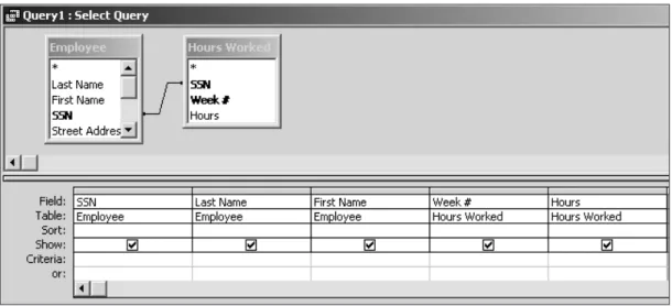
6. Create a Parameter query that shows the hours employees have worked. Have the Parameter query prompt for the week number. The output headings should be Last Name, First Name, Week #, and Hours. Do this only for the non-salaried workers. Use the table shown in Figure B-59 to work out your QBE grid on paper before creating your query.
Figure B-59 QBE grid template
Run the query with “2” when prompted for the Week #. Your output should look like that shown in Figure B-60.
Figure B-60 Number 6 query output
7. Create an update query that gives certain workers a merit raise. You must first create an additional table as shown in Figure B-61.
Figure B-61 MERIT RAISES table
Now make a query that adds the Merit Raise to the current Wage Rate for those who will receive a raise. When you run the query, you should be prompted with “You are about to update two rows.” Check the original WAGE DATA table to confirm the update. Use the table shown in Figure B-62 to work out your QBE grid on paper before creating your query.
Field Table Sort Show Criteria Or:
Figure B-62 QBE grid template
C
REATINGR
EPORTSDatabase packages let you make attractive management reports from a table’s records or from a query’s output. If you are making a report from a table, the Access report generator looks up the data in the table and puts it into report format. If you are making a report from a query’s output, Access runs the query in the background (you do not control this or see this happen) and then puts the output in report format.
There are three ways to make a report. One is to handcraft the report in the Design View, from scratch. This is tedious and is not shown in this tutorial. The second way is to use the Report Wizard, during which Access leads you through a menu-driven construction. This method is shown in this tutorial. The third way is to start in the Wizard and then use the Design View to tailor what the Wizard produces. This method is also shown in this tutorial.
Creating a Grouped Report
This tutorial assumes that you can use the Wizard to make a basic ungrouped report. This section of the tutorial teaches you how to make a grouped report. (If you cannot make an ungrouped report, you might learn how to make one by following the first example that follows.)
AT THE KEYBOARD
Suppose that you want to make a report out of the HOURS WORKED table. At the main Objects menu, start a new report by choosing Reports—New. Select the Report Wizard and select the HOURS WORKED table from the drop-down menu as the report basis. Select OK. In the next screen, select all the fields (using the >> button), as shown in Figure B-63.
Field Table Update to Criteria
T
utorial B
T
utorial B
Figure B-63 Field selection step in the Report Wizard
Click Next. Then tell Access that you want to group on Week # by double-clicking that field name. You’ll see that shown in Figure B-64.
Figure B-64 Grouping step in the Report Wizard
Click Next. You’ll see a screen, similar to the one shown in Figure B-65, for Sorting and for Summary Options.
Figure B-65 Sorting and Summary Options step in the Report Wizard
Because you chose a grouping field, Access will now let you decide whether you want to see group subtotals and/or report grand totals. All numeric fields could be added, if you choose that option. In this example, group subtotals are for total hours in each week. Assume that you do want the total of hours by week. Click Summary Options. You’ll get a screen similar to the one in Figure B-66.
Figure B-66 Summary Options in the Report Wizard
Next, follow these steps:
1. Click the Sum box for Hours (to sum the hours in the group).
2. Click Detail and Summary. (Detail equates with “group,” and Summary with “grand total for the report.”)
3. Click OK. This takes you back to the Sorting screen, where you can choose an order-ing within the group, if desired. (In this case, none is.)
T
utorial B
T
utorial B
4. Click Next to continue.
5. In the Layout screen (not shown here) choose Stepped and Portrait.
6. Make sure that the “Adjust the field width so all fields fit on a page” check box is unchecked.
7. Click Next.
8. In the Style screen (not shown), accept Corporate. 9. Click Next.
10. Provide a title—Hours Worked by Week would be appropriate. 11. Select the Preview button to view the report.
12. Click Finish.
The top portion of your report will look like that shown in Figure B-67.
Figure B-67 Hours Worked by Week report
Notice that data is shown grouped by weeks, with Week 1 on top, then a subtotal for that week. Week 2 data is next, then there is a grand total (which you can scroll down to see). The subtotal is labeled “Sum,” which is not very descriptive. This can be changed later in the Design View. Also, there is the apparently useless italicized line that starts out “Summary for ‘Week ...” This also can be deleted later in the Design View. At this point, you should select File—Save As (accept the suggested title if you like). Then select File—Close to get back the Database window. Try it. Your report’s Objects screen should resemble that shown in Figure B-68.
To edit the report in the Design View, click the report title, then the Design button. You will see a complex (and intimidating) screen, similar to the one shown in Figure B-69.
Figure B-69 Report design screen
The organization of the screen is hierarchical. At the top is the Report level. The next level down (within a report) is the Page level. The next level or levels down (within a page) are for any data groupings you have specified.
If you told Access to make group (summary) totals, your report will have a Report Header area and end with a Grand Total in the Report Footer. The report header is usually just the title you have specified.
A page also has a header, which is usually just the names of the fields you have told Access to put in the report (here, Week #, SSN, and Hours fields). Sometimes the page num-ber is put in by default.
Groupings of data are more complex. There is a header for the group—in this case, the value of the Week # will be the header; for example, there is a group of data for the first week, then one for the second—the values shown will be 1 and 2. Within each data grouping is the other “detail” that you’ve requested. In this case, there will be data for each SSN and the related hours.
Each Week # gets a “footer,” which is a labeled sum—recall that you asked for that to be shown (Detail and Summary were requested). The Week # Footer is indicated by three things:
1. The italicized line that starts =Summary for ... 2. The Sum label
3. The adjacent expression =Sum(Hours)
The italicized line beneath the Week # Footer will be printed unless you eliminate it. Similarly, the word “Sum” will be printed as the subtotal label unless you eliminate it. The “=Sum(Hours)” is an expression that tells Access to add up the quantity for the header in question and put that number into the report as the subtotal. (In this example, that would be the sum of hours, by Week #.)
T
utorial B
T
utorial B
Each report also gets a footer—the grand total (in this case, of hours) for the report. If you look closely, each of the detail items appears to be doubly inserted in the design. For example, you will see the notation for SSN twice, once in the Page Header and then again in the Detail band. Hours are treated similarly.
The data items will not actually be printed twice, because each data element is an object in the report; each object is denoted by a label and by its value. There is a representation of the name, which is the boldface name itself (in this example, “SSN” in the page header), and there is a representation in less-bold type for the value “SSN” in the Detail band.
Sometimes, the Report Wizard is arbitrary about where it puts labels and data. If you do not like where the Wizard puts data, the objects containing data can be moved around in the Design View. You can click and drag within the band or across bands. Often, a box will be too small to allow full numerical values to show. When that happens, select the box and then click one of the sides to stretch it. This will allow full values to show. At other times, an object’s box will be very long. When that happens, the box can be clicked, re-sized, then dragged right or left in its panel to reposition the output.
Suppose that you do not want the italicized line to appear in the report. Also suppose that you would like different subtotal and grand total labels. The italicized line is an object that can be activated by clicking it. Do that. “Handles” (little squares) appear around its edges, as shown in Figure B-70.
Figure B-70 Selecting an object in the Report Design View
Press the Delete key to get rid of the selected object.
To change the subtotal heading, click the Sum object, as shown in Figure B-71.
Figure B-71 Selecting the Sum object in the Report Design View
Click again. This gives you an insertion point from which you can type, as shown in Figure B-72.
Figure B-72 Typing in an object in the Report Design View
Change the label to something like Sum of Hours for Week, then hit Enter, or click some-where else in the report to deactivate. Your screen should resemble that shown in Figure B-73.
You can change the Grand Total in the same way.
Finally, you’ll want to save and then print the file: Select File—Save, then select File— Print Preview. You should see a report similar to that in Figure B-74 (top part is shown).
Figure B-74 Hours Worked by Week report
Notice that the data are grouped by week number (data for Week 1 is shown) and subto-taled for that week. The report would also have a grand total at the bottom.
Moving Fields in the Design View
When you group on more than one field in the Report Wizard, the report has an odd “staircase” look. There is a way to overcome that effect in the Design View, which you will learn next. Suppose that you make a query showing an employee’s last name, street address, zip code, and wage rate. Then you make a report from that query, grouping on last name, street address, and zip code. (Why you would want to organize a report in this way is not clear, but for the moment, accept the organization for the purpose of the example.) This is shown in Figure B-75.
T
utorial B
T
utorial B
Then, follow these steps: 1. Click Next.
2. You do not Sum anything in Summary Options.
3. Click off the check mark by “Adjust the field width so all fields fit on a page”. 4. Select Landscape.
5. Select Stepped. Click Next. 6. Select Corporate. Click Next.
7. Type a title (Wage Rates for Employees). Click Finish.
When you run the report, it will have a “staircase” grouped organization. In the report that follows in Figure B-76, notice that Zip data is shown below Street Address data, and Street Address data is shown below Last Name data. (The field Wage Rate is shown subordi-nate to all others, as desired. Wage rates may not show on the screen without scrolling.)
Figure B-76 Wage Rates for Employees grouped report (Wage Rate not shown)
Suppose that you want the last name, street address, and zip all on the same line. The way to do that is to take the report into the Design View for editing. At the Database window, select “Wage Rates for Employees” Report and Design. At this point, the headers look like those shown in Figure B-77.
Your goal is to get the Street Address and Zip fields into the last name header (not into the page header!), so they will then print on the same line. The first step is to click the Street Address object in the Street Address Header, as shown in Figure B-78.
Figure B-78 Selecting Street Address object in the Street Address header
Hold down the button with the little hand icon, and drag the object up into the Last Name Header, as shown in Figure B-79.
Figure B-79 Moving the Street Address object to the Last Name header
Do the same thing with the Zip object, as shown in Figure B-80.
Figure B-80 Moving the Zip object to the Last Name header
To get rid of the header space allocated to the objects, tighten up the “dotted” area between each header. Put the cursor on the top of the header panel. The arrow changes to something that looks like a crossbar. Click and drag it up to close the distance. After both headers are moved up, your screen should look like that shown in Figure B-81.
Figure B-81 Adjusting header space
Your report should now resemble the portion of the one shown in Figure B-82.
T
utorial B
T
utorial B
I
MPORTINGD
ATAText or spreadsheet data is easily imported into Access. In business, importing data hap-pens frequently due to disparate systems. Assume that your healthcare coverage data is on the Human Resources Manager’s computer in an Excel spreadsheet. Open the software application Microsoft Excel. Create that spreadsheet in Excel now, using the data shown in Figure B-83.
Figure B-83 Excel data
Save the file, then close it. Now you can easily import that spreadsheet data into a new table in Access. With your Employee database open and Tables object selected, click New and click Import Table, as shown in Figure B-84. Click OK.
Find and import your spreadsheet. Be sure to choose Microsoft Excel as Files of Type. Assuming that you just have one worksheet in your Excel file, your next screen looks like that shown in Figure B-85.
Figure B-85 First screen in the Import Spreadsheet Wizard
Choose Next, and then make sure you select the check box that says First Row Contains Column Headings, as shown in Figure B-86.
T
utorial B
T
utorial B
Store your data in a new table, do not index anything (you’ll see this in the next screen of the Wizard), but choose your own primary key, which would be SSN, as chosen in Figure B-87.
Figure B-87 Choosing a primary key field in the Import Spreadsheet Wizard
Continue through the Wizard, giving your table an appropriate name. After the table is imported, take a look at it and its design. (Highlight the Table option and use the Design but-ton.) Note the width of each field (very large). Adjust the field properties as needed.
F
ORMSForms simplify adding new records to a table. The Form Wizard is easy to use and can be performed on a single table or on multiple tables.
When you base a form on one table, you simply identify that table when you are in the Form Wizard set-up. The form will have all the fields from that table and only those fields. When data is entered into the form, a complete new record is automatically added to the table. But what if you need a form that includes the data from two (or more) tables? Begin (counterintuitively) with a query. Bring all tables you need in the form into the query. Bring down the fields you need from each table. (For data-entry purposes, this probably means bringing down all the fields from each table.) All you are doing is selecting fields that you want to show up in the form, so you make no criteria after bringing fields down in the query. Save the query. When making the form, tell Access to base the form on the query. The form will show all the fields in the query; thus, you can enter data into all the tables at once.
Suppose that you want to make one form that would, at the same time, enter records into the EMPLOYEE table and the WAGE DATA table. The first table holds relatively permanent data about an employee. The second table holds data about the employee’s starting wage rate, which will probably change.
The first step is to make a query based on both tables. Bring down all the fields from both tables into the lower area. Basically, the query just gathers up all the fields from both tables into one place. No criteria are needed. Save the query.
The second step is to make a form based on the query. This works because the query knows about all the fields. Tell the form to display all fields in the query. (Common fields— here, SSN—would appear twice, once for each table.)
Forms with Subforms
You can also make a form that contains a subform. This application would be particularly handy for viewing all hours worked each week by employee. Before you create a form that contains a subform, you must form a relationship between the tables. Suppose that you want to show all the fields from the EMPLOYEE table, and for each employee, you want to show the hours worked (all fields from the HOURS WORKED table).
Join the Tables
To begin, first form a relationship between those two tables by joining them: Choose the Tables object and then choose Tools-Relationships. The Show Table dialog box will pop up. Add the EMPLOYEE table and the HOURS WORKED table. Drag your cursor from the SSN field in the EMPLOYEE table to the SSN field in the HOURS WORKED table. Another dialog box will pop up, as shown in Figure B-88.
Figure B-88 The Edit Relationships dialog box
Click the Join Type button, and choose Number 2: Include ALL records from ‘Employee’ and only those records from ‘Hours Worked’ where the joined fields are equal, as shown in Figure B-89.
T
utorial B
T
utorial B
Click OK, then click Create. Close the Edit Relationships window and save the changes.
Create the Form and Subform
To create the form and subform, first create a simple, one-table form using the Form Wizard on the EMPLOYEE table. Follow these steps:
1. In the Forms Object, choose Create form by using Wizard.
2. Make sure the table Employee is selected under the drop-down menu of Tables/Queries.
3. Select all Available Fields by clicking the right double-arrow button. 4. Select Next.
5. Select Columnar layout. 6. Select Next.
7. Select Standard Style. 8. Select Next.
9. When asked, “What title do you want for your form?”, type Employee Hours. 10. Select Finish.
After the form is complete, click on the Design View, so your screen looks like the one shown in Figure B-90.
Make sure the Toolbox window is showing on the screen (Figure B-91). If it is not visible, select View—Toolbox. (The Toolbox may also appear as a toolbar for some students.)
Figure B-91 The Toolbox window
Click the Subform/Subreport button (6throw, button on right) and, using your cursor, drag
a small section next to the State, Zip, Date Hired, and US Citizen fields in your form design. As you lift your cursor, the Subform Wizard will appear, as shown in Figure B-92.
Figure B-92 The Subform Wizard
Follow these steps to create data in the subform: 1. Select the button Use Existing Tables and Queries. 2. Select Next.
3. Under Tables/Queries, choose the HOURS WORKED table, and bring all fields into the Selected Fields box by clicking the right double-arrow button.
T
utorial B
T
utorial B
5. Select the Choose from a list radio button. 6. Select Next.
7. Use the default subform name. 8. Select Finish.
Now you will need to adjust the design so all fields’ data are visible. Go to the Datasheet View, and click through the various records to see how the subform data changes. Your final form should resemble the one shown in Figure B-93.
Figure B-93 The Employee Hours form with the Hours Worked subform
Create a Switchboard Form
If you want someone who knows nothing about Access to run your Access database, you can use the Switchboard Manager to create a Switchboard form to simplify their work. A Switchboard form provides a simple, user-friendly interface that has buttons to click to do certain tasks. For example, you could design a Switchboard with three buttons: one for the Employee Hours Worked form, one for the Wage Rates for Employees report, and one for the Hours Worked by Week report. Your finished product will be a page showing three buttons. Each button can be clicked to open either the form, or one of the two reports. To design that Switchboard, use the following steps:
1. Remain on the Forms Object. 2. Select Tools.
3. Select Database Utilities. 4. Select Switchboard Manager.
5. A screen will prompt you with the question, “The Switchboard Manager was unable to find a valid switchboard in this database. Would you like to create one?” Click Yes.
The Switchboard Manager screen will open, as shown in Figure B-94. Leaving the Switchboard (Default) highlighted, click the Edit button.
Figure B-94 The Switchboard Manager screen
In the Edit Switchboard page, you will create three new items on the page. Click the New button. In the Edit Switchboard Item box, insert the following three items of data (as shown in Figure B-95):
1. Text: Employee Hours Worked Form 2. Command: Open Form in Add Mode 3. Form: Employee Hours
Click OK when you are finished.
Figure B-95 The Edit Switchboard Item screen
You will repeat this procedure two more times (that is, click the New button in the Edit Switchboard Page). Next, insert the following data:
1. Text: Wage Rate for Employees Report 2. Command: Open Report
3. Report: Wage Rate for Employees
Click OK when you are finished. Then, repeat the procedure (that is, click the New but-ton in the Edit Switchboard Page) and insert the following data:
T
utorial B
T
utorial B
2. Command: Open Report 3. Report: Hours Worked by Week
Click OK when you are finished. At this point, your Edit Switchboard screen should look like Figure B-96.
Figure B-96 The Edit Switchboard Page
Click the Close button, and then click the Close button again.
You can test the Switchboard by clicking the Switchboard in the Forms Objects. It should look like that shown in Figure B-97.
T
ROUBLESHOOTINGC
OMMONP
ROBLEMSAccess beginners (and veterans!) sometimes create databases that have problems. Common problems are described here, along with their causes and corrections.
1. “I saved my database file, but it is not on my disk! Where is it?”
You saved to some fixed disk. Use the Search option of the Windows Start button. Search for all files ending in “.mdb” (search for *.mdb). If you did save it, it is on the hard Drive (C:\) or on some network drive. (Your site assistant can tell you the drive designators.) Once you have found it, use Windows Explorer to copy it to your diskette in Drive A:. Click it, and drag to Drive A:.
Reminder: Your first step with a new database should be to Open it on the intended drive, which is usually Drive A: for a student. Don’t rush this step. Get it right. Then, for each object made, save it within the current database file.
2. “What is a ‘duplicate key field value’? I’m trying to enter records into my Sales table. The first record was for a sale of product X to customer #101, and I was able to enter that one. But when I try to enter a second sale for customer #101, Access tells me I already have a record with that key field value. Am I only allowed to enter one sale per customer!?”
Your primary key field needs work. You may need a compound primary key— CUSTOMER NUMBER and some other field or fields. In this case, CUSTOMER NUMBER, PRODUCT NUMBER, and DATE OF SALE might provide a unique combination of values—or you might consider using an INVOICE NUMBER field as a key.
3. “My query says ‘Enter Parameter Value’ when I run it. What is that?”
This symptom, 99 times out of 100, indicates you have an expression in a Criteria or a Calculated Field, and you misspelled a field name in the expression. Access is very fussy about spelling. For example, Access is case sensitive. Furthermore, if you put a space in a field name when you define the table, then you must put a space in the field name when you reference it in a query expression. Fix the typo in the query expression. This symptom infrequently appears when you have a calculated field in a query, and you elect not to show the value of the calculated field in the query output. (You clicked off the Show box for the calculated field.) To get around this problem, click Show back on.
4. “I’m getting a fantastic number of rows in my query output—many times more than I need. Most of the rows are duplicates!”
This symptom is usually caused by a failure to link together all tables you brought into the top half of the query generator. The solution is to use the manual click-and-drag method. Link the fields (usually primary key fields) with common values between tables. (Spelling of the field names is irrelevant because the link fields need not be spelled the same.)
5. “For the most part, my query output is what I expected, but I am getting one or two duplicate rows.”
You may have linked too many fields between tables. Usually only a single link is needed between two tables. It’s unnecessary to link each common field in all combina-tions of tables; usually it’s enough to link the primary keys. A layman’s explanation for why over-linking causes problems is that excess linking causes Access to “overthink” the problem and repeat itself in its answer.
On the other hand, you might be using too many tables in the query design. For exam-ple, you brought in a table, linked it on a common field with some other table, but then did not use the table. You brought down none of its fields and/or you used none of its fields in query expressions. Therefore, get rid of the table, and the query should still work. Try doing this to see whether the few duplicate rows disappear: Click the unneeded table’s header in the top of the QBE area and press the Delete key. 6. “I expected six rows in my query output, but I only got five. What happened to the
other one?”
Usually this indicates a data-entry error in your tables. When you link together the proper tables and fields to make the query, remember that the linking operation joins records from the tables on common values (equal values in the two tables). For exam-ple, if a primary key in one table has the value “123”, the primary key or the linking field in the other table should be the same to allow linking. Note that the text string “123” is not the same as the text string “123 ”—the space in the second string is considered a character too! Access does not see unequal values as an error: Access moves on to consider the rest of the records in the table for linking. Solution: Look at the values entered into the linked fields in each table and fix any data-entry errors. 7. “I linked fields correctly in a query, but I’m getting the empty set in the output. All I
get are the field name headings!”
You probably have zero common (equal) values in the linked fields. For example, suppose you are linking on Part Number (which you declared as text): In one field you have part numbers “001”, “002”, and “003”, and in the other table part numbers “0001”, “0002”, and “0003”. Your tables have no common values, which means no records are selected for output. You’ll have to change the values in one of the tables. 8. “I’m trying to count the number of today’s sales orders. A Sigma query is called for.
Sales are denoted by an invoice number, and I made this a text field in the table design. However, when I ask the Sigma query to ‘Sum’ the number of invoice numbers, Access tells me I cannot add them up! What is the problem?”
Text variables are words! You cannot add words, but you can count them. Use the Count Sigma operator (not the Sum operator): Count the number of sales, each being denoted by an invoice number.
9. “I’m doing Time arithmetic in a calculated field expression. I subtracted the Time In from the Time Out and I got a decimal number! I expected 8 hours, and I got the number .33333. Why?”
[Time Out] – [Time In] yields the decimal percentage of a 24-hour day. In your case, 8 hours is one-third of a day. You must complete the expression by multiplying by 24: ([Time Out] – [Time In]) * 24. Don’t forget the parentheses!
10. “I formatted a calculated field for currency in the query generator, and the values did show as currency in the query output; however, the report based on the query output does not show the dollar sign in its output. What happened?”
Go into the report Design View. There is a box in one of the panels representing the calculated field’s value. Click the box and drag to widen it. That should give Access enough room to show the dollar sign, as well as the number, in output.
11. “I told the Report Wizard to fit all my output to one page. It does print to just one page. But some of the data is missing! What happened?”
T
Access fits the output all on one page by leaving data out! If you can stand to see the output on more than one page, click off the “Fit to a Page” option in the Wizard. One way to tighten output is to go into the Design View and remove space from each of the boxes representing output values and labels. Access usually provides more space than needed.
12. “I grouped on three fields in the Report Wizard, and the Wizard prints the output in a staircase fashion. I want the grouping fields to be on one line! How can I do that?” Make adjustments in the Design View. See the Reports section of this tutorial for instruction.
13. “When I create an Update query, Access tells me that zero rows are updating, or more rows are updating than I want. What is wrong?”
If your Update query is not correctly set up, for example, if the tables are not joined properly, it will either try not to update anything, or it will update all the records. Check the query, make corrections, and run it again.
14. “After making a Summation Query with a Sum in the Group By row and saving that query, when I go back to it, the Sum field now says Expression, and Sum is put in the field name box. Is this wrong?”
Access sometimes changes that particular statistic when the query is saved. The data remains the same, and you can be assured your query is correct.