HAL Id: halshs-00620825
https://halshs.archives-ouvertes.fr/halshs-00620825
Submitted on 8 Sep 2011HAL is a multi-disciplinary open access archive for the deposit and dissemination of sci-entific research documents, whether they are pub-lished or not. The documents may come from teaching and research institutions in France or abroad, or from public or private research centers.
L’archive ouverte pluridisciplinaire HAL, est destinée au dépôt et à la diffusion de documents scientifiques de niveau recherche, publiés ou non, émanant des établissements d’enseignement et de recherche français ou étrangers, des laboratoires publics ou privés.
Global modelisation and local characteristics of French
periurban spatial organization
Matthieu Drevelle
To cite this version:
Matthieu Drevelle. Global modelisation and local characteristics of French periurban spatial organi-zation. 17th European Colloquium on Quantitative and Theoretical Geography, Sep 2011, Athènes, Greece. pp.130-138. �halshs-00620825�
Global modelisation and local characteristics of French periurban
spatial organization
Matthieu DREVELLE1
1
PhD Student, UMR Géographie-Cités - University Paris 1 Panthéon la Sorbonne – Transamo, France, Email : [email protected]
ABSTRACT
This paper aims at finding global rules about periurban spatial organization in France according to three main indexes: intensity of periurbanisation, range of periurban commutes and concentration of periurban flows. Comparing all French agglomerations with more than 5.000 jobs, we have highlighted links between the population of these agglomerations and our three indexes. That is why this research proposes statistical models to determinate periurban spatial organization according to agglomeration size.
Moreover, observing the spatial repartition of residuals, we have highlighted some local characteristics in this organization. Using geographical information systems, we have tried, in this paper, to explain these local characteristics by geographic facts and historic resilience.
KEYWORDS
Periurbanisation, urban spatial structure, spatial analysis, GIS, France
1. INTRODUCTION
No one can deny that the face of our cities has been transformed by periurbanisation during the last decades. Most of the urban studies community agrees to say that today’s cities cannot be reduced to the historic core or to the morphological agglomeration. In fact, our cities can be compared to an archipelago (Beaucire, Emangard, 1995) composed of a central continent (the historical core of the agglomeration) and a lot of islands (the periurban areas) which are attracted by the continent. Nevertheless, the boundaries of this “urban archipelago” are hard to define because we can use many different definitions. This study does not aim at giving a new definition of cities: “it’s too big, we have many chance to make mistakes” (Perec, 1974), its purpose is to answer the two following questions:
- Does periurbanisation spatial characteristics (intensity, range and concentration) are linked with the size of agglomeration? Can we find a “global rule” for periurban spatial organization?
- Can we observe local characteristics in the spatial organization of periurbanisation? And how can we explain these characteristics by history and geography?
The periurbanisation process is well studied in geography; many recent works focus on new urban and suburban structures in the world (Boiteux-Orain, Huriot, 2001 ; Bertaud, Malpezzi, 2004). Moreover, a lot of monographic works have been done on specific periurban areas, such as Paris’ metropolitan area (Berger, 2004), Rennes (Baudelle et al., 2007) or Toulouse (Rougé, 2009). Commuting is also a well studied subject with some major comparative works (Newman & Kenworthy, 1999). Nevertheless, in France, only a few researches have tried to compare a great number of agglomerations. Le Jeannic (1997) has done a very interesting research on the demographical evolution of periurban population and on the mobility between periurban areas and core agglomerations for all the French agglomerations. But his work is now quite old (proposing an analysis on the 1962-1990 period) and it does not really deal with periurban spatial organization. Wiel (1999) has calculated some indexes of periurban spatial organization for many cities, but his work as not been updated and does not concern all the French agglomerations. A new approach is to study periurban morphology at a fine scale and to characterize the form of all periurban islands (Emangard, 2008) but this method requires a priori the analysis of spatial structure at a more large scale.
In this paper, we have studied periurban spatial organization for all the 354 French agglomerations with more than 5.000 jobs, using the methods developed by quantitative geography (Haggett, 1973; Pumain, Saint Julien, 1997) and GIS spatial analysis. We have also tried to explain our results with thematic and historical geography (Braudel, 1990; Planhol, 1988).
2. METHODOLOGY
Define periurban spatial characteristics in France requires to qualify periurbanisation. As we said previously the concept of ‘periurbanisation’ has multiple definitions.In this research, we do not choose to use INSEE’s (French Institute of statistics) official definition of “periurban area” which is old (1999) and inappropriate to our work because it gives a periurban attribute to places and not to people. In fact, this official definition is based on a threshold of municipalities’ workers working in the agglomeration (40%); so many periurban commuters are excluded of the definition (if the threshold of 40% is not reached). Our own definition of periurbanisation is based on people’s behavior: is considered as a periurban everyone who works in an agglomeration and lives outside of this agglomeration within a range of 100km (which is the official maximum distance of “daily mobility”). With this definition, the influence area of an agglomeration is not necessary a continuous area and a municipality could be in the influence area of many agglomerations.
Our definition of agglomeration is the INSEE’s one (named “pole urbain” and defined as morphological agglomeration with more than 5000 jobs). Because of this morphological definition, the “pole urbain” contains the historical center and most of the suburban subcenters. Assuming a monocentic urban structure in French metropolitan areas ((Boiteux-Orain, Huriot, 2001), our work doesn’t focus on outlying subcenters which represent a very low part of metropolitan jobs (Aguilera, Mignot, 2004).
All our quantitative work and our definition of periurban is based on an individualized database of daily commuting in France in 2007 (RGP INSEE 2007). Methodology of this paper is divided in three steps:
2.1. Building indexes to define periurbanisation
Our analysis is based on three indexes: the intensity, the range and the concentration of periurbanisation. The intensity index (I) aims at quantifying the proportion of periurban people for each agglomeration. It is calculated by dividing the number of people working in the agglomeration and living outside by the total job number in the agglomeration.
The range index (R) is used to know how far periurban people are living from their job and by extension how big is the influence area of the agglomeration. This index is the median (Rmedian), the first (RQ1) and the third quartile (RQ3) of periurban commutes length. Commutes lengths are calculated for each periurban people as the Euclidian distance between the place of residence’s townhouse and the place of work’s townhouse.
The concentration index (C) aims at showing how the periurbanisation is concentrated in a few number of periurban towns, or how it is dispersed in a lot of periurban villages. This index is based on the weight of commuters’ flows: we have calculated for each agglomeration a Gini coefficient (Gini, 1909) (which is an inequality index) on these weighted flows. The nearer the index is to 1, the more unequal the flows are, so the more concentrated in a few municipalities periurbanisation is. On the contrary, the nearer the index is to 0, the more equal the flows are, so the more dispersed in all the attracted municipalities periurbanisation is.
These indexes have been calculated for all the agglomerations in order to make regressions and to highlight global rules for periurban spatial organization.
2.2. Observing local and spatial characteristics
As our statistical model based on agglomeration size is not perfect, we have decided to do a spatial analysis on the previous regressions’ residuals. We have classified the residuals of the different regressions in different classes and plotted them on a map. Observing the repartition of agglomeration with high or low residuals could give keys to highlight local characteristics of periurban spatial structure. In order to complete our local analysis, we have also calculated a Kernel density (Rosenblatt, 1956; Parzen, 1962) on the residuals with a range of 100km. Smoothing is often used in geography to transform punctual data into a continuous area (Grasland, 1999). The range of 100km has been chosen in order to fit with the “daily mobility” definition. This step aims at identifying and to observing areas with high intensity of positive or negative residuals.
2.3. Trying to explain local characteristics
A last step in this local analysis is to compare our quantitative results with the analysis of thematic geography and historical geography. In fact, we assume the postulate that the actual organization of cities can be explained by the resilience of territory organization. In this work, this step is only based on map observation and comparison, but a further analysis in a future research could use a statistical approach such as Geographically Weighted Regression (Charlton, Fortheringham, 2009).
3. RESULTS
3.1. Range, intensity and dispersion of periurbanisation are correlated to city’s population
Our first research hypothesis is that intensity, range and concentration of periurbanisation are correlated to the population of agglomeration. This hypothesis is checked by our statistical work for the 354 French agglomerations. Indeed, we get good results for our three statistical models with a R² around 0,5. Some of these results are patently obvious: the median range of periurban commutes increases with core agglomeration size. One interesting information is that the median range, but also the first and the third quartiles, are correlated with the logarithm of agglomeration population (see table 1) and that the interquartile coefficient is globally around 2,5. These regressions allow to model the repartition of periurban population around the core agglomeration: it allows us to draw three circles around the centre of city containing respectively 25%, 50% and 75% of the periurban commuters.
Charts 1 & 2: Median range and intensity of periurbanisation according to agglomeration size
The two other statistical regressions give less intuitive results and permit to precise our model of periurban people’s spatial repartition. The periurban intensity model gives us the percentage of periurban commuters. It is a power regression (or log-log regression) and it gives a surprising result: the bigger the city is, the lower the intensity of periurbanisation is. This phenomenon, traducing a strong residential attractiveness of big agglomerations, might be explained by the greater number of services offered to people living in big agglomerations. Moreover, because of congestion, these central services are harder to access to periurban people. On the contrary, in smaller agglomerations, central area can be reached quicker, so it might be more attractive to live in periurban area to benefit lower housing price and natural land. Nevertheless, this intensity index is a relative number: if the percentage of periurban is lower in big agglomerations, their number is greater. As a matter of fact, we can identify a linear relation between the population of core city and the number of periurban people with a very good R² (0,92 with all the cities and 0,78 if we exclude Paris)(see table 1).
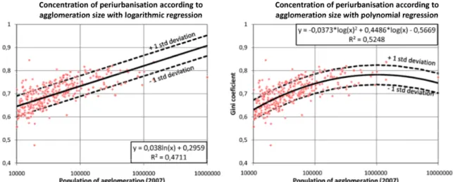
The last regression (on concentration index, based on Gini’s coefficient) also gives interesting results. We can observe that periurbanisation is more concentrated in big agglomerations than in smaller ones. In other
words, the commuters’ flows are more concentrated in a few number of municipalities in big agglomeration and more equally distributed in the smaller ones (even if the number of municipalities attracted by an agglomeration grows exponentially with the size of the agglomeration)(see table 1). Nevertheless, if a logarithmic regression gives good results for agglomerations until 1.000.000 inhabitants (see chart 3), we can observe that the Gini’s coefficient is never higher than 0,85. In fact, it seems to exist a threshold around 1.000.000 inhabitants. After that, we can see that the Gini’s coefficient seems to stabilize or slowly decline (even if we have only one very big agglomeration in our study). That’s why we can propose a second model for concentration using logarithms and polynomial regression (chart 4). This second model has a better R² and seems closer to the reality, so we can conclude that after one or two million inhabitants in the core agglomeration, the number of attracted municipalities is so huge that the concentration index cannot continue to grow.
Charts 3 & 4: Concentration of periurbanisation according to agglomeration size with logarithmic regression and
polynomial regression
As a first conclusion, it is possible to model periurban spatial structure of French agglomerations according to their population. Indeed, our statistical models are able to determine the intensity of periurbanisation, the number of periurban commuters and their spatial localization: distance to the core agglomeration and level of concentration in a few number of municipalities (see table 1). Nevertheless, even if the precision of our models is quite good (with a R² around 0,5), it seems to be very interesting to see the spatial repartition of residuals. It will lead us to know if some local characteristics can influence our model.
Index Formula (x=population of the core
agglomeration)
Adjusted R² Range of periurbanisation (1st quartile) RQ1 = 3,3293*log(x) - 6,3461 0,554
Range of periurbanisation (median) Rmedian = 4,4825*log(x) - 6,6195 0,5276
Range of periurbanisation (3rd quartile) RQ3 = 5,2561*log(x) - 1,4689 0,3531
Intensity of periurbanisation I = 3,76662x-0,19951 0,4858
Number of periurban people P = 0,099x + 5737,5 0,7833
Concentration of periurbanisation (Gini coefficient) C = -0,0373*log(x)2 + 0,4486*log(x) - 0,5669
0,5248
Number of municipalities attracted N = 4,2939x0,3901 0,78
3.2. Behind global rules: the local characteristics of periurbanisation in France
If the statistical models have shown global rules of periurban spatial organization, the cartography of residuals is useful to highlight local characteristics independently of agglomerations size. The results of this step of our research are quite surprising because a spatial structure of residuals clearly appears for the difference indexes, but each index has its own specific spatial organization. These organizations appear in the following maps where we have plotted all our agglomerations with a specific color representing residuals. Agglomerations who are represented in the previous graphs (part 3.1) between the two lines of “+ 1 standard deviation” and “- 1 standard deviation” are plotted in white because we estimate that they are explained by the model. Agglomerations with a negative residual bigger than one standard deviation are plotted in blue and these with a positive residual higher than one standard deviation are plotted in red. A smoothing function (using Kernel density) permits to observe regional areas with negative or positive residuals (see map1).
Map 1: Localisation of residuals of the statistical models of periurbanisation
The first results of this analysis is that intensity of periurbanisation is greater in the North-West of France (especially in Picardie, Normandie and Bretagne), in the east (North of Alsace) and around Lyon. On the contrary the intensity of periurbanisation is lower in a diagonal starting from North-East to South-West (known in France as the “empty diagonal”) and in the South-East (the Alps and the East part of Mediterranean coast). The repartition of residuals for the concentration model also shows a clear spatial organization. Periurbanisation is more concentrated along a diagonal running from west (Bretagne) to South-East (mediterrean coast) and more dispersed in North, East and South-West. The residuals of range model have a less apparent spatial structure. However, we can see that the median range of periurban commutes is lower in the Nort-East border and in the valley of Rhine and Rhone.
3.3. Explaining local characteristics of periurbanisation: geographic facts or historical resilience?
One of our hypotheses to explain this phenomenon is that periurban spatial organization is linked to historical resilience. In other word, we think that historical or geo-historical facts (such as distance between cities, boundaries of municipalities or rural population before rural-urban migration) could explain a part of today’s periurban spatial organization.
The first spatial repartition we want to explain is the concentration index. This index is based on commuters flows between municipalities and a problem of scale appears. In fact, French municipalities have different areas, so a high concentration index could just be caused by a territory with wide municipalities. To cancel this effect, we have done the map of municipalities’ density in France and we have observed that areas with a high density of municipalities are areas with low periurban concentration (see Map 2). So we have decided to add this parameter (density of municipalities) in our previous statistical model and we have obtained a very good result (R²=0,743, see the formula in Map 6). Moreover the residuals map of this new model reveals a new spatial organization highlighting a greater concentration of periurbanisation in the Rhone valley, in the west and the north-east of France and in the north-west of Paris (see map 3). This analysis prevents us against the danger of using non regular geographical entities and shows how geo-historical facts could affect statistical index. In fact the boundaries of municipalities have not been created by chance: they have been created during the French revolution of 1789 but are based on old parishes (which size was depending of agrarian system).
Map 2: Density of municipalities compared to the residuals of the concentration model.
Map 3: Location of residuals of our new concentration statistical model (population of agglomeration + density of
Area of municipality does not appear as a significant element in the spatial repartition of range (R²=0,002) except in Arcachon (on the South-West coast) where it clearly appears that the high range of periurban commutes is due to the extreme size of municipalities around the agglomeration (more than 10 times the average area of French municipalities). Nonetheless we have another geographical hypothesis to explain residuals: the urban system and concurrence between cities. This hypothesis is based on the Reilly law: if an agglomeration is far from all the others, it can extend its influence area wildly, on the contrary if an agglomeration is in a dense urban system, its influence area enters in concurrence with other agglomerations. We have not been able to link with a good correlation coefficient the range of periurbanisation and the density of the urban system. But the comparison between the map of density of urban system and the map of median range model’s residuals reveals that some areas, where range of periurbanisation is lower than the model (North of France, East and Rhone valley), are also areas with a very dense urban system: the only exception is Normandy (see Map 4).
Map 4: Density of municipalities compared to the residuals of the concentration model.
Map 5: Density of rural people in 1861 compared to the residuals of the intensity model.
The last residuals repartition to explain is the intensity index. For us, the differences in the spatial repartition of periurbanisation intensity might be explained by “rural tradition” of territories, which could influence the wish of people to live out of agglomerations. In other words, territories with a high density of rural population before the “rural exodus” may have conserved a rural tradition, so more people would like to settle in the country land. To prove our hypothesis, we have used data from the French census of 1861 to know the density of rural population before rural-urban migration. Results are quite conclusive,
we observe a very good similarity between the residuals map of intensity model and the map of density of rural population in 1861 (see map 5). Of course this comparison is not enough to prove that “rural tradition” is a cause of high periurban intensity but it shows the resilience of historic facts in nowadays urban organization.
4. CONCLUSION
Periurban spatial organization in France can be explained by core agglomeration population: the intensity of periurbanisation decreases with the number of inhabitants in the agglomeration although the range of commuting and the concentration of periurban people increase with agglomeration size. We have also highlighted some local or regional characteristics. So, as a final result of our research, we are able to present a global statistical model of periurban spatial structure and a synthesis map which shows the local particularities of this structure (see map 6).
Moreover, we have shown that a part of these local characteristics seems to be explained by geographical facts and historical resilience, such as urban system density or importance of rural population during the 19th century. So it may be interesting to do further research on resilience in periurban spatial organization.
Map 6: Synthesis map of local characteristics of periurban spatial organization in France
5. ACKNOWLEDGMENTS
I would like to thank Francis BEAUCIRE, my PhD director, and all the PhD students of the “tempête dans
les transports” brain storming team for their precious advices and their help. Thanks to Fred, Marion and
Alice for the review.
6. REFERENCES
AGUILERA A., MIGNOT D., “Urban sprawl, polycentrism and commuting”, in Urban Public Economic
BAUDELLE G., DARRIS G., OLLIVRO J., PIHAN J., “Les conséquences d’un choix résidentiel périurbain sur la mobilité : pratiques et représentations des ménages”, in Cybergeo : European Journal of
Geography, article 287, 2007
BERTAUD A., MALPEZZI S., 2003, The Spatial Distribution of Population in 48 World Cities:
Implications for Economies in Transition, University of Wisconsin.
BEAUCIRE F., EMANGARD P.H., Dynamique spatiale de l’agglomération nantaise, CETE ouest, 1995 BERGER M., Les périurbains de Paris. De la ville dense à la métropole éclatée ? CNRS Éditions, Espaces et Milieux, 2004, 317 p.
BOITEUX-ORAIN C, HURIOT J.M., 2001, “Modéliser la suburbanisation. Succès et limites de la microéconomie urbaine”, in Economie (1991-2003), n°2001-02, LATEC, Université de Bourgogne. BRAUDEL F., L’identité de la France, Flammarion, Paris, 1990, 553p.
CHARLTON M., FOTHERINGHAM S., 2009, Geographically weighted regression, National Centre for Geocomputation, Maynooth, Ireland.
EMANGARD P.H., Diversité des formes de la périurbanisation en France, Journées ESIU, Paris – La Défense, 2008
GINI C., Concentration and dependency ratios, 1909
GRASLAND C., 1999, “Lissage cartographique et animation spatio-temporelle: quelques réfléxions théoriques et méthodologiques”, in Travaux de l’institut de Géographie de Reims, n°101-104, pp.83-104. HAGGET P., L’analyse spatiale en géographie humaine, Armand Colin, collection U, 1973, 390p. LE JEANNIC T., “Trente ans de périurbanisation : extention et diluation des villes”, In Economie et
statistiques, n°307, sept 1997, pp 21-41
NEWMAN P., KENWORTHY J., Sustainability and Cities: Overcoming Automobile Dependence, Island Press, Washington, D.C., USA, 1999.
PARZEN E., “On estimation of a probability density function and mode”, in Annals of Mathematical
Statistics, 33: pp. 1065–1076, 1962
PLANHOL X., Géographie historique de la France, Fayard, Paris, 1988, 635p.
PUMAIN D., SAINT-JULIEN T., L'analyse spatiale. 1. Localisations dans l'espace. Paris, Armand Colin, Col. Cursus, Série Géographie, 1997, 167 p.
ROUGE L., “L’installation périurbaine entre risque de captivité et opportunités d’autonomisation”, in
Articulo - Journal of Urban Research [Online], 5, 2009
ROSENBLATT M., “Remarks on some nonparametric estimates of a density function”, in Annals of
Mathematical Statistics 27: pp. 832–837, 1956
WIEL M., Forme et intensité de la périurbanisation et aptitude à la canaliser, Paris, DRAST, 1999.- 74 p., annexes, cartes.