Frequency Selection for Reflectometry-based Soft Fault Detection using Principal Component Analysis

HAL Id: hal-02295328

https://hal-centralesupelec.archives-ouvertes.fr/hal-02295328

Submitted on 12 Mar 2020

HAL is a multi-disciplinary open access

archive for the deposit and dissemination of

sci-entific research documents, whether they are

pub-lished or not. The documents may come from

teaching and research institutions in France or

abroad, or from public or private research centers.

L’archive ouverte pluridisciplinaire HAL, est

destinée au dépôt et à la diffusion de documents

scientifiques de niveau recherche, publiés ou non,

émanant des établissements d’enseignement et de

recherche français ou étrangers, des laboratoires

publics ou privés.

Frequency Selection for Reflectometry-based Soft Fault

Detection using Principal Component Analysis

Nour Taki, Wafa Ben Hassen, Nicolas Ravot, Claude Delpha, Demba Diallo

To cite this version:

Nour Taki, Wafa Ben Hassen, Nicolas Ravot, Claude Delpha, Demba Diallo. Frequency Selection

for Reflectometry-based Soft Fault Detection using Principal Component Analysis. Prognostics and

Systems Health Management Conference (PHM-Paris 2019), May 2019, Paris, France. �hal-02295328�

Frequency Selection for Reflectometry-based Soft

Fault Detection using Principal Component Analysis

Nour TAKI 1,2 1. _{CEA, LIST} 2. _{L2S, CNRS UMR 8506-} CentraleSupelec - Univ. Paris

Sud

91192 Gif-sur-Yvette, France nour.taki@cea.fr

Wafa BEN HASSEN CEA, LIST 91192 Gif-sur-Yvette, France wafa.benhassen@cea.fr Nicolas RAVOT CEA, LIST 91192 Gif-sur-Yvette, France nicolas.ravot@cea.fr Claude DELPHA*

Laboratoire des Signaux et Systèmes (L2S)

CNRS UMR 8506 - CentraleSupelec - Univ. Paris Sud

91192 Gif Sur Yvette, France claude.delpha@l2s.centralesupelec.fr

Demba DIALLO

Group of Electrical Engineering of Paris(GeePs) CNRS UMR 8507, CentraleSupelec,

Univ. Paris Sud, Sorbonne Univ. 91192 Gif Sur Yvette, France demba.diallo@geeps.centralesupelec.fr Abstract—This paper introduces an efficient approach to

select the best frequency for soft fault detection in wired networks. In the literature, reflectometry method has been well investigated to deal with the problem of soft fault diagnosis (i.e. chafing, bending radius, pinching, etc.). Soft faults are characterized by a small impedance variation resulting in a low amplitude signature on the corresponding reflectograms. Accordingly, the detection of those faults depends strongly on the test signal frequency. Although the increase of test signal frequency enhances the soft fault “spatial” resolution, it provides signal attenuation and dispersion in electrical wired networks. In this context, the proposed method combines reflectometry-based data and Principal Component Analysis (PCA) algorithm to overcome this problem. To do so, the Time Domain Reflectometry (TDR) responses of 3D based-models of faulty coaxial cable RG316 and shielding damages have been simulated at different frequencies. Based on the obtained reflectograms, a PCA model is developed and used to detect the existing soft faults. This latter permits to determine the best frequency of the test signal to fit the target soft fault.

Keywords—Time domain reflectometry, Principal component analysis, Wire diagnosis, Soft fault, Frequency selection, Statistical Chart.

I. INTRODUCTION

ire diagnosis addresses the problem of electrical fault detection, localization and characterization. Various arising technologies are used to resolve this issue [1]. However, the lights are spotted widely on the Time Domain Reflectometry (TDR) method, which utilizes a fast rise time pulse and deals with most industry’s wiring issues [2]. Based on the principle of radar, it injects a high-frequency test signal down the wire under test and records the echoes created at each impedance discontinuity such as junctions and faults. The correlation of the obtained signal to the injected one is known as a reflectogram where each peak corresponds to an impedance singularity. The energy of the test signal may be well attenuated due to the presence of cable inhomogeneity, junctions, coupling, splices, etc., and detecting electrical faults becomes complex. This

complexity increases in presence of soft faults (i.e. chafing, bending radius, pinching).

In fact, soft faults are characterized by a small impedance variation leading to a low amplitude signature on the corresponding reflectogram. Moreover, in noisy environments such as vibration, high temperature, crosstalk, etc., those faults detection encounter several difficulties. As a solution, further development is needed to make the reflectometry method sensitive enough to detect and locate soft faults. In this context, several post-processing methods have been proposed in [3–5]. A Self-Adaptive Correlation Method (SACM) where the gain is automatically adjusted depending on the fault signature is proposed in [3]. A Signature Magnification by Selective Windowing (SMSW) method is proposed in [4] to select the critical zone based on a predetermined window. In [5], a fusion approach of several post-processing results is proposed where a probabilistic model is developed and used to detect the soft fault. Although interesting methods have been proposed to enhance soft fault diagnosis, they are prone to test signal attenuation and dispersion phenomena.

Moreover, the signature of the soft fault may be invisible on the corresponding reflectogram since the front and back of the fault may cancel each other out when the time width of the test signal is greater than the length of the soft fault [6]. Hence, the choice of the test signal bandwidth is very important and affects the diagnosis performance. Although bandwidth increases the resolution for detecting soft faults, it provides more attenuation. Thereby, a compromise between those two quantities should be defined.

In this paper, a new approach for the frequency selection in the case of soft fault diagnosis is proposed. Indeed, the TDR response has been simulated for several soft fault cases at four different frequencies after which principal component analysis (PCA) is applied to the obtained data where a multivariate statistical test is used to select the proper frequency.

The remaining of the paper is organized as follows. Section II illustrates the used model in our approach and the simulation results. Section III focuses on the PCA theory and how it is used for Fault Detection and Diagnosis (FDD). Section IV describes the proposed approach for the frequency selection and the obtained results. Section V concludes the paper.

II. SOFT FAULT DETECTION BASED ON TDR Reflectometry techniques rely on the propagation of electrical signals in a transmission line. Indeed, the way in which the signals propagate is related to the physical characteristics of the line. The behavior of the line, at the electrical level, can provide information on the existing faults. The basics of line theory are presented here in order to establish the link between the electrical response of a line and the characteristics of the faults. An RLCG circuit constituted of the following parameters models the high-frequency propagation in a transmission line: resistance R (Ohm/m), inductance L (Henry/m), capacitance C (Farad/m) and conductance G (Siemens/m). Equations (1) and (2) indicate the variation of the parameters L and C as a function of frequency where 𝜇₀ is the vacuum magnetic permeability and 𝜇𝑟 is the relative permeability of the

conductor. D and d are the outer and inner conductor diameters respectively. The parameter 𝜀₀ defines the air permittivity and 𝜀𝑟 is the relative permittivity of the

dielectric [7]. In the case of loss-free propagation R=G=0. L=𝜇𝑟 𝜇0 𝜋

acos (

𝐷 𝑑

)

(1) C= 𝜋 𝜀𝑟 𝜀0 acosh(𝐷_𝑑) (2)

In [8], the complex propagation constant (3) is defined as a function of the radian frequency 𝜔= 2𝜋f (radian/s) and its imaginary part (4), 𝛽 (radian/m), defines the phase constant where Im(.) is the imaginary part operator. The solution of the Telegraph’s equations gives (5), the characteristic impedance Zc (Ohm) of the line.

The presence of an impedance discontinuity along the line generates reflected waves. Equation (6) gives the reflection coefficient

Γ

f at any discontinuity along the line

where Zf is the fault impedance [3]. This parameter is of high importance in the principle of reflectometry.

𝛾(ω)= √(R+jωL)(G+jωC) (3) 𝛽= Im(𝛾) (4) Zc=

√

R+jωL G+jωC (5)

Γ

f

=

Z_f - Z_c Zf + Zc (6)

In fact, the propagation velocity (7) and the spatial resolution (8) enabled by a test signal vary with the frequency as shown [9]: vp(f)= 2πf β (7) ∆

=

_𝐵vp 𝑇 (8)

where 𝐵𝑇 is the bandwidth of the test signal.

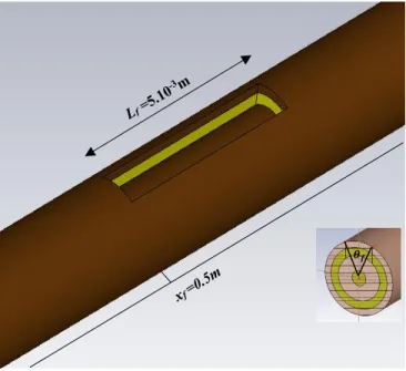
In the process of understanding the behavior of a point-to-point cable in presence of soft faults, in a noiseless environment, an RG316 coaxial cable with 1m length is modeled using 3D simulation software (CST). Then, shielding damage is introduced as shown in Fig.1 and is defined by three parameters: the length Lf, the position xf

and the angular cutaways 𝜃𝑓. In this case, the length of the

fault Lf = 5.10-3m and the position is set at the middle of the

cable (xf = 0.5m).

The construction specifications of this cable are given in Table I. Using the formula in (5), Zc⋍ 45Ω.

Fig. 1. Fault parameters

TABLEI.RG316CONSTRUCTIONSPECIFICATIONS

Description Material Diameter

Core Copper 0.51 10-3_m

Dielectric PTFE 1.52 10-3_m

Shield Copper 2.06 10-3_m

Jacket FEP 2.59 10-3_m

First, the healthy cable signature reflectograms are simulated at four different bandwidths, where the bandwidth is defined from DC to a maximal frequency 𝑓𝑚𝑎𝑥. The

angular cutaways parameter 𝜃𝑓 is set to one of the three

values: 45°, 90° and 180°. The cable is excited using a Gaussian pulse with different maximal frequencies (1GHz, 2GHz, 3GHz and 4GHz).

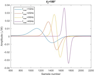
Figures 2, 3 and 4 represent the signature of the shielding damage with angular cutaways 𝜃𝑓=45°, 𝜃𝑓=90°

and 𝜃𝑓=180° respectively and this, for the different maximal

frequencies. It is obvious that the signature amplitude and the resolution of the soft fault increase with the frequency as described in (8). Since frequency changes with velocity as described in (7), a shift between the signatures of the same fault at different frequencies is observed on the reflectograms.

As shown in Table II, both the fault severity and the excitation frequency causes the peak amplitudes of the fault signatures to be increased.

Fig. 2. Soft fault signatures for 𝜃𝑓= 45°

Fig. 3. Soft fault signatures for 𝜃𝑓= 90°

Fig. 4. Soft fault signatures for 𝜃𝑓= 180°

TABLEII.THEDIFFERENTFAULTSIGNATUREPOSITIVEPEAKS

Frequency (GHz) Amplitude (√w.10 -3₎ A45° A90° A180° 1 2.79 9.04 10.13 2 3.69 15.93 18.62 3 5.41 24.40 27.98 4 6.89 31.67 36.22

III. PCA FOR FDD

A. PCA principle

PCA [10] is a multivariate data-driven statistical modeling technique. It uses information redundancy in a high-dimensional correlated input space to project the original data set into a lower dimensional subspace defined by the principal components (PCs). The main research objective of PCA is the dimensionality reduction of the problem. It considers, in several cases, a substantial variability percentage in the data that can be interpreted using a limited number of components.

The analysis begins with the data matrix X ∈ ℝn×m_which

consists of m variables with n observations (n>m). The element xij is the ith observation of the jth variable. In PCA,

before processing, X is normalized into Xc [11]. Precisely,

each vector of Xc is calculated as:

𝒙𝒋𝒄=

𝒙𝒋− 𝜇𝑥_𝑗

𝜎𝑥_𝑗 (9)

where 𝜇𝑥_𝑗and 𝜎𝑥_𝑗 are the mean and the standard deviation

values of the jth _{vector 𝒙}

𝒋 respectively.

PCA depends on eigenvalue decomposition of the Xc

covariance or correlation matrix. Let C denotes the correlation matrix of Xc as follows:

C= 1

𝑛−1

X

c

T

X

c (10)

where (. )𝑇_{is the transpose operator.}

By means of Singular Value Decomposition (SVD), one can write C as:

C= P

ΛP

T

_{, where PP}

T

_{= P}

T

_{P= I}

mxm (11)

where P= [p1,p2,…, pm] ∈ ℝm×m is the PCA loading matrix

such that its columns pj are the eigenvectors of the

correlation matrix C. Vectors pj are orthonormal and they

are also known as the weight vectors. The matrix Λ is diagonal with the elements {λj} for 1 ≤ j≤ m are the

eigenvalues of C sorted in descending order.

According to [12-14], PCA decomposes the data matrix into two parts; the first explains the system variation while the second encapsulates the residual information (noise):

X

c

= TP

T

= T

l

P

lT

+

𝑇̃

𝑃̃

T (12)

where T, highlighting the relationship between the samples in Xc, stands for the principal component score matrix and

the superscript (~) is the residual matrix operator.

The selection of the number l (with

l

≤ m) of principal components to retain is considered as a matter of high importance. Different methods had been used for this purpose [15-16]. Cumulative Percent Variance (CPV) method [17] is used in this paper to set _l as the number of PCs cumulatively contributing to more than 90 percent of the data variability:

CPV (

l

)

=

∑ λk l 1 ∑ λm _k 1

≥ 90%

(13) B. PCA-based FDD

Fault detection is to figure out if a fault has occurred or not. The first step here is to have the normal operating data upon which the PCA model will be established. This model is utilized then to examine new measurement data. Two statistical methods are used here. The Q (or Squared Prediction Error SPE) and the Hotelling T2 _{statistics [13].}

PCA-based FDD includes two phases. First, the training phase where data are collected during fault-free operation and PCA model is developed. Second, the monitoring phase, i.e., fault detection is handled using the monitoring statistics and fault diagnosis will be managed through contribution plots.

New measurements Xnew will be projected into the

framework spanned with the loading matrix Pl.. The new scores Tnew and the residual 𝑇̃new are calculated according to

(14) and (15). Then, the Q and T2 _{statistical values in (16)} and (17) are used for evaluating the fault presence. They display the variations that are not interpretable by the retained PCs in the residual and the principal subspaces respectively.

T

new

= X

new

P

_l (14)

𝑇̃

new

= X

new

(I- P

_l

P

_lT

)

(15)

Q= 𝑇̃

new

𝑇̃

newT (16)

T

2

₌

∑ (

tj λ_j

)

2 l 1 (17)

where tj is the jth column vector of

T

new

.

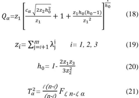
In the case of an abnormal event, the Q and T2 _statistic values will be greater than the confidence limits 𝑄𝛼 and 𝑇𝛼2

respectively. Those limits are calculated using the healthy original data that constructs the PCA model:

𝑄𝛼=𝑧1[ 𝑐𝛼 √2𝑧2ℎ02 𝑧1 + 1 + 𝑧₁ℎ₀(ℎ₀−1) 𝑧12 ] 1 ℎ0 (18)

𝑧

_𝑖

= ∑

m_j=l+1

λ

_ji

i= 1, 2, 3 (19) ℎ0= 1- 2𝑧_3𝑧1𝑧3 2 2 (20) 𝑇𝛼2= l (n-l)_(n-l)

F

_{l, n-l, α} (21)

where 𝑐𝛼 is the critical value of the normal distribution at 𝛼

significance level and

F

_{l, n-l, α} is the Fisher–Snedecor distribution critical value.

If at a specific sample the Q or T2 _{value falls outside the} confidence limit, then there exists an abnormality. We can inspect the inputs (responsible variables) that highly influence their residual. Contribution plots are used for this purpose.

IV. RESULTS AND DISCUSSIONS

The reference, healthy performance, representation of the data is given by (22). X is formed up of four variables. Each variable 𝑅̅_{𝑓𝐺𝐻𝑧} is a column vector of the matrix and corresponds to the cable healthy TDR response at the frequency f (1GHz, 2GHz, 3GHz and 4GHz respectively). The number of samples for each variable 𝑅̅𝑓𝐺𝐻𝑧 is 4101, i.e.,

X ∈ ℝ4101×4.

= [𝑅̅1𝐺𝐻𝑧 𝑅̅2𝐺𝐻𝑧 𝑅̅3𝐺𝐻𝑧 𝑅̅4𝐺𝐻𝑧] (22)

The obtained data matrix X is then used for the construction of the PCA model according to (9), (10), (11) and (12).

Table III shows the PCs coefficients, also known as loadings. Table IV indicates that the cumulative variance of the first two scores is 98.64% that is greater than the lower limit. This implies that the observed variables are highly correlated. Using (13), the data is well described by a two principal component model. Thus, l is equal to two.

The new measurement data set corresponds to the faulty modeled cases. It has four vectors such that Xnew=[x1 x2 x3

x4]. Each one of the four variables is a concatenated vector of the fault signature data (𝜃𝑓= 45°, 𝜃𝑓= 90° and 𝜃𝑓= 180°)

at the same frequency. The new data matrix is defined as follows: = [ 𝑅̅45°1𝐺𝐻𝑧 𝑅̅45°2𝐺𝐻𝑧 𝑅̅45°3𝐺𝐻𝑧 𝑅̅45°4𝐺𝐻𝑧 𝑅̅90°1𝐺𝐻𝑧 𝑅̅90°2𝐺𝐻𝑧 𝑅̅90°3𝐺𝐻𝑧 𝑅̅90°4𝐺𝐻𝑧 𝑅̅180°1𝐺𝐻𝑧 𝑅̅180°2𝐺𝐻𝑧 𝑅̅180°3𝐺𝐻𝑧 𝑅̅180°4𝐺𝐻𝑧 ] (23) = [x1 x2 x3 x4]

where 𝑅̅_𝜃°_𝑓 describes the fault signature data vector with angular cutaways 𝜃 and frequency f.

The constructed PCA model is then used to check the new measurement data. To do so, the differences between the new measurement data and their projections into the constructed model are then subjected to the Q and Hoteling’s T2 _{statistical tests. The 95% confidence limits of} those tests are calculated according to (18-21). Thus, 𝑄_𝛼= 22.25 and 𝑇𝛼2= 26.92.

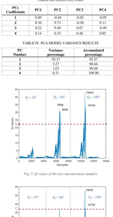
According to (14-17), the SPE and the T2 _{values of each} new measurement sample are calculated. Figures 5 and 6 present the Q and the T2 _{control charts respectively, with the} dashed red line representing the 95% confidence limit. It is shown that 𝑄𝛼 have been exceeded by some samples (6508,

6630, 10620 and 10730) and 𝑇𝛼2 by the samples (10620 and

10730). This indicates that faults have occurred.

Plotting the contribution charts in Fig. 7 and Fig. 8 of the indicated faulty samples permits to know the variable (x1, x2, x3 or x4) that highly influences their Q and T2 values. Thereby, the selection of the relevant frequency is performed by Q and Hotelling T2 _{control tests. The sample} 6508 in Fig.7 is related only to the Q test whereas the sample 10620 in Fig.8 is related to the two tests. The contribution of the first variable x1 is almost neglected with respect to the other variables; hence, it does not appear in the plots.

If we look at Figures 5, 7 and 8, we can draw the following concluding remarks:

- for 𝜃𝑓= 45°, the fault cannot be detected whatever the

frequency.

- for 𝜃𝑓= 90° and 𝜃𝑓= 180°, the faults are undetectable at

1, 2 or 3GHz frequencies.

- for 𝜃𝑓= 90° and 𝜃𝑓= 180°, at 4GHz, the faults are

clearly detected.

However, Figures 6, 7 and 8 show that the fault is only detectable for 𝜃𝑓= 180° at 4GHz.

Thanks to the simulation results of a 1m length RG316 coaxial cable with a shielding damage with 3 severity levels (45°, 90° and 180°), the combination of reflectometry and PCA coupled to Q and T2 _{statistics shows that:}

- the highest frequency (4GHz) leads to the best fault detection capability for the two largest severities if Q test is used and the largest severity detection if T2 _{test is used.}

- for the lowest fault severity, the Q and T2 _{in the PCA} framework fail to detect the fault.

- Q test is more suitable than T2 _{to be used in our case} study since it is able to detect more faults.

TABLEIII.EIGENVECTORS

PCs Coefficients PC1 PC2 PC3 PC4 1 0.89 -0.44 -0.02 -0.05 2 0.36 0.73 -0.56 0.11 3 0.22 0.48 0.67 -0.49 4 0.14 0.15 0.46 0.85 TABLEIV.PCAMODELVARIANCERESULTS

PC Number Variance percentage Accumulated percentage 1 95.37 95.37 2 3.27 98.64 3 1.03 99.68 4 0.31 100.00

Fig. 5. Q values of the new measurement samples

Fig. 6. T² values of the new measurement samples

𝜃𝑓= 45° 𝜃𝑓= 90° 𝜃𝑓= 180°

𝜃𝑓= 45° 𝜃𝑓= 90° 𝜃𝑓= 180°

Fig. 7. Contribution plot of the sample 6508

Fig. 8. Contribution plot of the sample 10620

V. CONCLUSION

This paper introduces an efficient approach to select the best frequency bandwidth for soft fault detection in wired networks based on a judicious combination of reflectometry and Principal Component Analysis.

In practice, the expert configures and calibrates the Vector Network Analyzer (VNA) at a given frequency and records the healthy cable measurement. Measurements at the same frequency as before will be done on a faulty cable. Analysis of the measurements will be established at this frequency on the PC. If the fault is not detected, the expert must redo the measurements at a higher frequency and so on. Therefore, there is a loss of information and time in addition to the subjectivity of the decision-making.

The proposed method permits to configure and calibrate the VNA at different frequencies. It performs measurements on different frequencies for the healthy case. After which the PCA model is established. It performs the real-time measurements at different frequencies. If a difference is detected between the model and the real-time data, the contribution of each variable (i.e. frequencies) to this difference is calculated. The algorithm then chooses the most relevant frequency to monitor the non-frank defect in

the perspective of a prognosis. The advantages are thus time saving and objectivity of the decision-making. Furthermore, monitoring the evolution of defects in the prognosis perspective.

The simulation results are in coherence with the previously known rule that for short cables, the higher the frequency, the better it is for the fault detection. In future works, this approach will be applied to another set of cables with different operating conditions and different fault types. Other statistics will also be evaluated to cope with the detection of incipient faults.

REFERENCES

[1] F. Auzanneau, "Wire troubleshooting and diagnosis: review and perspectives", Progress In Electromagnetics Research B, vol. 49, pp. 253-279, 2013.

[2] C. Furse, Y. C. Chung, C. Lo, P. Pendayala. "A critical comparison of reflectometry methods for location of wiring faults", Journal of Smart

Structures and Systems, 2(1), pp. 25-46, 2006.

[3] S. Sallem, N. Ravot, "Self-adaptive correlation method for soft defect detection in cable by reflectometry", Proceeding of 2014 IEEE

Sensors Conference, 2114-2117, Valencia, Spain, 2014.

[4] S. Sallem, N. Ravot, "Self-adaptive correlation method for soft defect detection in cable by reflectometry". In Sensors, 2014 IEEE, pp. 2114-2117, 2014.

[5] W. Ben Hassen, M. Gallego Roman, B. Charnier, N. Ravot, A. Dupret, A. Zanchetta, F. Morel, "Embedded OMTDR Sensor for Small Soft Fault Location on Aging Aircraft Wiring Systems",

Procedia Engineering, vol. 168, pp. 1698-1701, 2016.

[6] L. A. Griffiths, R. Parakh, C.Furse, B. Baker, "The invisible fray: A critical analysis of the use of reflectometry for fray location". IEEE

Sensors Journal, 6(3), 697-706, 2006.

[7] W. Ben Hassen, N. Ravot, A. Dupret, A. Zanchetta, F. Morel, L. Pillon, C. Chuc, "OMTDR-based embedded cable diagnosis for mutliple fire zones detection and location in aircraft engines". In

Sensors, 2017 IEEE (pp. 1-3), 2017.

[8] M. B. Steer, "Microwave and RF design: a systems approach".

SciTech Pub, 2010.

[9] M. Kafal, A. Cozza, L. Pichon, "Locating faults with high resolution using single-frequency TR-MUSIC processing". IEEE Transactions

on Instrumentation and Measurement, 65(10), 2342-2348, 2016.

[10] R. Penha, J.W. Hines, "Using principal component analysis modeling to monitor temperature sensors in a nuclear research reactor". In

Proceedings of the 2001 Maintenance and Reliability Conference

(MARCON 2001), Knoxville, TN, 2001.

[11] H. Wang, Z. Song, P. Li, "Fault detection behavior and performance analysis of principal component analysis based process monitoring methods". Industrial & Engineering Chemistry Research, 41(10), 2455-2464, 2002.

[12] T. J. McAvoy, "Intelligent "Control" applications in the Process Industries". Annual Reviews in Control, 26, pp.75-86, 2002. [13] D. Slišković, R. Grbić, Ž. Hocenski, "Multivariate statistical process

monitoring". Tehnicki Vjesnik-Technical Gazette, 19(1), 33-41, 2012. [14] J. Harmouche, C. Delpha, D. Diallo, "Incipient fault detection and

diagnosis based on Kullback–Leibler divergence using principal component analysis: Part I". Signal Processing, 94, 278-287, 2014. [15] G. Diana, C. Tommasi, "Cross-validation methods in principal

component analysis: a comparison. Statistical Methods and Applications", 11(1), 71-82, 2002.

[16] R. B. Cattell, "The scree test for the number of factors". Multivariate

behavioral research, 1(2), 245-276, 1966.

[17] J. L. Horn, "A rationale and test for the number of factors in factor analysis". Psychometrika, 30(2), 179-185, 1965.