HAL Id: hal-01557077
https://hal.archives-ouvertes.fr/hal-01557077
Submitted on 5 Jul 2017
HAL is a multi-disciplinary open access
archive for the deposit and dissemination of
sci-entific research documents, whether they are
pub-lished or not. The documents may come from
teaching and research institutions in France or
abroad, or from public or private research centers.
L’archive ouverte pluridisciplinaire HAL, est
destinée au dépôt et à la diffusion de documents
scientifiques de niveau recherche, publiés ou non,
émanant des établissements d’enseignement et de
recherche français ou étrangers, des laboratoires
publics ou privés.
Distributed under a Creative Commons Attribution| 4.0 International License
Multiscale analysis of genome-wide replication timing
profiles using a wavelet-based signal-processing
algorithm
Benjamin Audit, Antoine Baker, Chun-Long Chen, Aurélien Rappailles,
Guillaume Guilbaud, Hanna Julienne, Arach Goldar, Yves
d’Aubenton-Carafa, Olivier Hyrien, Claude Thermes, et al.
To cite this version:
Benjamin Audit, Antoine Baker, Chun-Long Chen, Aurélien Rappailles, Guillaume Guilbaud, et
al..
Multiscale analysis of genome-wide replication timing profiles using a wavelet-based
signal-processing algorithm.
Nature Protocols, Nature Publishing Group, 2013, 8 (1), pp.98-110.
�10.1038/nprot.2012.145�. �hal-01557077�
IntroDuctIon
Replication of eukaryotic genomes is an essential process that guaran-tees the accurate copying of genetic information before cell division. The regulation of this process during the synthesis phase (S phase) of the cell cycle is fundamental for genome stability. Replication starts from a set of initiation loci, called replication origins, where two repli-cation forks are assembled and begin replicating DNA while proceeding in opposite directions, away from the loci; fork progression continues until two converging forks ‘collide’ at a terminus of replication1,2.
The DNA replication program in a cell is defined as the tempo-ral sequence of locus replication events during the S phase. The program depends on the locations of the replication origins, their activation times and the speed at which replication forks move along the DNA double helix. Among these parameters, the location of the active replication origins has been the subject of extensive experimental interest. In Saccharomyces cerevisiae, replication ori-gins are well defined by 100- to 150-bp-wide loci that present an 11-bp consensus sequence motif1,2. By contrast, the detection of replication origins in higher eukaryotes has proven to be more elu-sive. For many years, only tens of origins had been experimentally identified in metazoan genomes, including the human genome3,4, to be compared with the tens of thousands that are required to complete each replication cycle in mammals. The number of iden-tified origins has markedly increased owing to high-throughput approaches based on the purification of replication bubbles and of small nascent DNA strands5–11. For example, a few hundred replication origins were recently mapped over ≤1% of the human genome7,8, and several thousands were mapped over 60 and 120 Mb of the mouse and Drosophila genomes, respectively10.
Note that comparative analyses of experimentally determined replication origin data sets for the same organism proved to be rather disappointing with low overlap (from < 5 to < 25%), and this incon-sistency was observed even when the same technique was used8,9. The reasons for these discrepancies are still not known4, but they could be the result of insufficient origin DNA purification and amplification biases. Nevertheless, these analyses clearly point to the flexibility in replication origin usage across developmental stages and underline the importance of the local context, such as the chromatin state, the tran-scriptional activity and the activation patterns of neighboring replica-tion origins12–17. Although the principles of replication initiation are likely to be conserved across eukaryotes, they are complex and far from being fully understood, particularly in higher eukaryotes3,18–20.
The fact that robust methodologies exist to analyze the DNA rep-lication program averaged over large populations of cells contrasts with the extreme difficulty of identifying individual replication ori-gins19,21,22. Most methods of analysis of DNA replication programs consist of the initial sorting of cells according to their advancement in the cell cycle; for each locus, either the DNA contents of cells in the S and G1 phases, respectively, are compared or this comparison is performed between the amounts of newly synthesized DNA in two or more fractions of cells in the S phase19,21.
In all cases, at the end of the analysis, each locus is associated with a measure of the production of DNA as the S phase progresses, a measure that is assumed to be representative of the average rep-lication timing of the specific locus in the cell population under investigation. However, the exact relationship between changes in the extent of DNA production and the mean timing of replication
Multiscale analysis of genome-wide replication
timing profiles using a wavelet-based
signal-processing algorithm
Benjamin Audit
1,2, Antoine Baker
1,2, Chun-Long Chen
3, Aurélien Rappailles
4,6, Guillaume Guilbaud
4,6,
Hanna Julienne
1,2, Arach Goldar
5, Yves d’Aubenton-Carafa
3, Olivier Hyrien
4, Claude Thermes
3& Alain Arneodo
1,2 1Université de Lyon, Lyon, France. 2Laboratoire de Physique, Centre National de la Recherche Scientifique (CNRS), Limité Mixte de Recherche (LMR) 5672, Ecole Normale Supérieure de Lyon, Lyon, France. 3Centre de Génétique Moléculaire, CNRS Unité Propre de Recherche (UPR) 3404, Associée à l’Université Paris-Sud, Fédération de Recherche du CNAS (FRC) 3115, Gif-sur-Yvette, France. 4Institut de Biologie de l’Ecole Normale Supérieure, CNRS UMR8197, Institut National de la Santé et de la Recherche Médicale (INSERM) U1024, Paris, France. 5Commissariat à l’Énergie Atomique, iBiTecS, Gif-sur-Yvette, France. 6Present addresses: Institut Pasteur, Laboratoire Régulation Spatiale du Génome, Paris, France (A.R.), Medical Research Council (MRC) Laboratory of Molecular Biology, Cambridge, UK (G.G.). Correspondence should be addressed to B.A. (benjamin.audit@ens-lyon.fr).In this protocol, we describe the use of the lastWave open-source signal-processing command language (http://perso.ens-lyon.fr/ benjamin.audit/lastWave/) for analyzing cellular Dna replication timing profiles. lastWave makes use of a multiscale,
wavelet-based signal-processing algorithm that is based on a rigorous theoretical analysis linking timing profiles to fundamental features of the cell’s Dna replication program, such as the average replication fork polarity and the difference between replication origin density and termination site density. We describe the flow of signal-processing operations to obtain interactive visual analyses of Dna replication timing profiles. We focus on procedures for exploring the space-scale map of apparent replication speeds to detect peaks in the replication timing profiles that represent preferential replication initiation zones, and for delimiting u-shaped domains in the replication timing profile. In comparison with the generally adopted approach that involves genome segmentation into regions of constant timing separated by timing transition regions, the present protocol enables the recognition of more complex patterns of the spatio-temporal replication program and has a broader range of applications. completing the full procedure should not take more than 1 h, although learning the basics of the program can take a few hours and achieving full proficiency in the use of the software may take days.
along the S phase is usually not known. For example, regardless of the length of the S phase, the ratio between the DNA content in cells in the S phase and that of cells in the G1 phase (S/G1 ratio) is close to 2 at early-replicating loci, whereas it is close to 1 at late-replicating loci.
Today, replication timing profiles are available for several eukaryotic organisms ranging from yeast23 to Drosophila15,24,25 to mice26,27 and to humans28–35. These data have been extensively analyzed in relation to transcriptional activity, chromatin state and genomic features, such as gene density and GC content. In metazoa, significant correlations have been observed between loci that are replicated early in the S phase and regions that present a strong transcriptional activity, an open chromatin state, a high gene den-sity or a high GC content15,24–26,29,31,33,34.
Replication timing profiles have also been used to identify replica-tion domains along chromosomes. A frequently adopted approach is to look for constant timing regions (CTRs) using algorithms designed to delimit regions of locally flat profile, such as those devel-oped to analyze variation in genome copy number (microarray- based comparative genomic hybridization)22,26,27,29,32,36. Alternatively, timing transition regions (TTRs) have been extracted from replication timing profiles directly by looking for long, steep transition regions of constant slope33. Such segmentations of rep-lication timing profiles implicitly assume a crude dichotomous nature of replication domains, in which CTRs are regions of coordi-nated origin firings and the intervening TTRs are originless regions replicated by the unidirectional progression of a single fork26,27,33. Recent DNA-combing data have questioned these interpretations37. Here we propose a novel method for analyzing replication timing profiles that does not assume this dichotomy.
For humans, mice and Drosophila, genome-wide replication tim-ing data have been collected for several cell types25,31,33–35,38,39; this provides the opportunity to study changes in the replication program in relation to cell differentiation and across evolution-ary history. Evidence shows that each cell type presents specific replication timing patterns; in fact, different cell type–dependent timing patterns occur in the replication of more than half of the human and mouse genomes27,34. In that respect, cell differentiation is concomitant with global changes in replication timing profiles, and some cell type–specific timing patterns are conserved between corresponding cell types27,38,39.
Single-cell determination of the replication timing profile cannot be currently achieved experimentally. As mentioned above, replica-tion timing data are instead obtained from large cell populareplica-tions (thousands to millions), and thus they only determine a popula-tion’s average replication program. If we assume a nearly deter-ministic replication program, in which at each cell cycle nearly the same set of replication origins is used, and in which each replication origin fires at (roughly) the same time from cell cycle to cell cycle, then the average replication program reflects faithfully what occurs at the individual cell level. However, a growing body of evidence suggests that the replication program is stochastic in nature40–43 and that no two replication cycles actually occur via the same set of replication origins and the same firing times.
If we accept the stochasticity of the replication program, some care is therefore needed in interpreting mean replication timing profiles44–46. For instance, the gradient of the mean replication timing profile has been proposed as a possible measure of the rep-lication fork velocity23. However, this approximation holds true
only for a nearly deterministic replication program. In fact, as rep-lication forks propagate, the reprep-lication timing at a given locus depends not only on the local initiation properties, but also on the initiation properties of neighboring loci44,47. Replication origins have also been proposed to correspond to the minima of the mean replication timing profile23, but this intuitive claim turns out to be incorrect because of the confounding effect of passive replication by forks originating from nearby replication origins44–46. A careful and rigorous analysis is therefore necessary to measure replication kinetic parameters from mean replication timing profiles44,47,48. A very challenging ‘inverse’ problem is to infer the underly-ing initiation properties from the replication timunderly-ing data47,49,50. Preliminary studies suggest that the time-dependent rate of ori-gin activation averaged over the entire genome is conserved across eukaryotes49,51.
With the perspective of extracting information about the rep-lication program directly from the DNA sequence, our research group carried out an in silico analysis of the strand composition asymmetry, also called skew (a measure of the difference of nucle-otide compositions between the two complementary DNA strands), along the human genome in relation to replication52,53 and tran-scription54,55. We found evidence that the sign of the skew abruptly changed at known origins, presumably reflecting the inversion of replication fork polarity at these sites as expected at replication ori-gins from which emerge two divergent replication forks. We identi-fied more than a thousand putative replication origins where the skew showed a similar abrupt inversion. These origins border 663 genomic N-domains, which are so called because their skew profile has an N-like shape that is attributed to differences in the mutation rates between the complementary DNA strands associated with the replication process53,56–60. To the best of our knowledge, these data provide the largest set of human replication origin predictions available to date.
Overall, skew N domains have a mean length L = 1.2 ± 0.6 Mb and cover 29.2% of the human genome57,58. Notably, the putative origins at N-domain borders were also shown to be at the heart of a remarkable gene organization57: genes neighboring these bor-ders are abundant and broadly expressed, and their transcription is mainly directed away from the borders. These features (gene density, expression breadth, preferential gene orientation) weaken progressively as the distance between genes and these domain bor-ders increases. N-domain borbor-ders were hypothesized to be replica-tion origins active in the germ line, possibly specified by an open chromatin structure favorable for early replication initiation and permissive to transcription61. However, no data on germ-line rep-lication origins enabled us to test this hypothesis. The analysis of human replication timing data31 showed that a significant number of N-domain borders are initiation zones that replicate earlier than their surrounding regions during the S phase, whereas N-domain central regions replicate late56. These very promising results have been confirmed in recent analyses59,62 of newly available genome-wide replication timing data in several human cell types33–35,38,39. In contrast with the viewpoint that replication domains are CTRs, we have shown that skew N-domains correspond to U-shaped replication timing patterns (in which the derivative of the replica-tion timing is N-shaped) that are not specific to the germ line but are generally observed in multiple human cell types62. The early initiation zones bordering the replication timing U-domains have been found to be significantly enriched in open chromatin markers,
including the insulator-binding protein CTCF63,64, and to be prone to gene expression.
Analysis of genome-wide chromatin conformation capture (Hi-C) data65 has revealed a link between replication timing and spatial chromatin organization38. Further study has highlighted replication timing U-domains as self-interacting structural chromatin units62. Hence, the segmentation of the genome into replication U-domains coincides with the segmentation into topological domains identi-fied by the analysis of chromatin interaction data66. Together, these results make a compelling case that the ‘islands’ of open chromatin observed at replication timing U-domain borders are at the heart of a compartmentalization of chromosomes into chromatin units of independent replication and of coordinated gene transcription62.
We present here the original wavelet-based multiscale methodo-logy that we have developed for the analysis of replication timing data in order to extract information about the mechanisms under-lying the spatio-temporal replication program in higher eukaryo-tes35,37,59,62. Our approach takes advantage of the knowledge of the replication timing continuously along the chromosomes.
In accordance with rigorous mathematical arguments, we con-sider the timing values per se, but we also concon-sider the space deriva-tives (i.e., the local shape) of the timing profiles. In contrast with model-fitting strategies47,67, in this approach we extract informa-tion independently of any prior knowledge of parameters such as potential replication origin locations. By partitioning the genome on the basis of the apparent speed of replication (the inverse of the timing profile slope)37, we are in the position to question the reported absence of replication origins within TTRs26,27,33 and to determine the extent of origin synchrony within CTRs. Moreover, as explained in the theoretical background section, given reasonable assumptions, the described wavelet-based methodology enables us to extract fundamental parameters, such as the average replication fork polarity and the difference between the densities of replication origins and termination sites62.
In this protocol, we describe the main steps of this signal process-ing strategy when applied to mean replication timprocess-ing profiles in HeLa cells that have been fully calibrated to real time along the S phase37. Note that if this normalization is not possible, then replication time and speed estimates will not be absolute but will be relative to the total duration of the S phase. The absence of time calibration is a limitation to our protocol (as well as of any other method used so far), and so are the limited temporal and spatial resolutions of experimental replication timing data that are variable from one experiment to another. Our protocol has been implemented using LastWave (http://www.cmap.polytechnique. fr/~bacry/LastWave/), an open-source signal-processing command language. The PROCEDURE section is devoted to the description of the distinct LastWave commands and scripts that constitute the standard protocol for (i) loading an experimental timing profile, (ii) computing a space-scale map of the apparent speed of tion, (iii) detecting peaks in the timing profile as putative replica-tion origins and (iv) delineating replicareplica-tion timing U-domains.
Applications
The wavelet-based multiscale methods presented here have a broad range of applications, for example, in physics, geophysics and image processing68–71. In the context of the analysis of biological data60, they have been used by our group (i) to demonstrate the existence of long-range correlations in DNA sequences related to
the nucleosomal structure72–74, (ii) to characterize the organiza-tion of human and microbial genomes75–77, (iii) to analyze strand compositional asymmetry profiles in relation to transcription and replication58,78, (iv) to assist diagnosis in digitized mammograms79 and (vi) to determine the shape of chromosome territories from confocal microscopy images80,81. Finally, we are currently devel-oping novel procedures to define, from chromosome conforma-tion data65, an objective segmentation of the human genome into topological chromatin domains66, which will enable us to quanti-tatively assess the relationship between replication domains and chromatin domains.
Theoretical background
The central hypothesis at the basis of our approach to extracting fundamental clues about the spatio-temporal program of DNA replication from mean replication timing profiles is that the replica-tion fork speed v is constant. In this scenario, the spatio-temporal program of replication of one cell cycle is completely specified by the position xi and the firing time ti of the n activated bidirectional
replication origins Oi (refs. 44,47). Upon definition of Ti as the
ter-mination locus in which the replication fork coming from Oi meets the replication fork coming from Oi + 1 (Fig. 1), straightforward calculations lead to the space-time coordinates (yi, ui) for Ti:
y x x v t t u t t x x v i i i i i i i i i i = + + − = + + − + + + + 1 2 1 2 1 1 1 1 [( ) ( )] [( ) ( )/ ]
and to the replication timing profile r(x) and replication fork polar-ity p(x) around origin Oi (yi − 1≤x ≤yi):
r x( )= + −ti |x xi| /vandp x( )=sign(x x− i)
where sign(u) = + 1 if u ≥ 0 and = − 1 if u < 0. Finally, by using the Dirac function δ to represent origin locations δ(x − xi) and
termination sites δ(x − yi) (Fig. 1c), we obtain the following
fun-damental relationships: n d xr x p x d ( )= ( ) v d x r x d xp x i x xi i x yi 2 2 2 2 d ( )=d ( )=
∑
d( − )−∑
d( − ) In other words, we can extract, up to a multiplicative constant, the fork polarity p(x) (Fig. 1b) and the location of origins and of termination sites (Fig. 1c) by simply taking successive derivatives (equations (3) and (4)) of the timing profile r(x) (Fig. 1a).As mentioned, today’s experimental replication timing profile protocols require a large number of cells (millions), so that only population statistics data can be derived. Moreover, experimental timing profiles31,33–35,38,39 have a finite spatial resolution (tens of kb at best). For application to experimental replication data, as taking the spatial derivative commutes with statistical and spatial average, equations (3) and (4) remain valid after averaging:
d x r x x v p x x d 〈( )〉Cells,∆ = 〈 ( )〉Cells,∆ 1 (1) (1) (2) (2) (3) (3) (4) (4) (5) (5)
d x r x x v N x x N x x 2 2 2 d Cells Cells Ori CellsTer 〈 ( )〉 ,∆ = ( ,∆ ( )− ,∆ ( )) where 〈.〉Cells,∆x stands for the average over many cells and over the spatial resolution ∆x and NCellsOri ,∆x( )x and NCellsTer ,∆x( )x are the number of origins and termination sites, respectively, per unit length averaged over many cells and the spatial resolution of ∆x. Note that when the speed of the replication fork is inhomogeneous, but fork speed fluctuations do not depend either on replication (6) (6)
timing or on chromosomal position, then equations (5) and (6) remain valid, with v representing the average replication speed.
A concern about experimental data is the presence of noise. Strictly speaking, the derivative of a noisy profile is not defined and, correspondingly, the naive derivative of a profile based on the numerical difference between two successive samples is ill defined and numerically unstable. However, the derivative of a smoothed version of a noisy profile is well defined. In other words, the rate of signal variation has to be estimated over a sufficiently large number of data points. This objective can be achieved using the (continuous) wavelet transform (WT), which provides a powerful framework for the estimation of signal variations over different length scales68,69.
The WT is a space-scale analysis, which consists in expanding signals in terms of wavelets that are constructed from a single func-tion, the analyzing wavelet ψ, by means of dilations and transla-tions68,69,82,83: T f x a a f y x y a y y( )a[ ]( , )= a ( )y − −∞ +∞
∫
dwhere x and a ( > 0) are the space and scale parameters, respectively, and α is the normalization exponent. When using the derivatives of the Gaussian function, namely N(n)(x) = dnN(0)(x) / dxn, with
N( )0( )x 1 x2 2/ 2
= −
p e , then the WT of a profile f has the follow-ing property: T f x a d x N f x N n n n n a ( ) ( (− +1))[ ]( , )=
(
( )0 ∗)
( ) dEquation (8) shows that the WT computed with N(n) and normali-zation exponent α = − (n + 1) simply reduces to the nth derivative of the profile f smoothed by a dilated version N x
aN x a
a( )0( )=1 ( )0( / ) of the Gaussian function. The regularization (smoothing) process underlying the use of the WT is at the heart of various applications of the WT microscope as a very efficient multiscale technique to detect singularities (e.g., discontinuities) of functions68,69,82–84. Note that the norm of the rescaled Gaussian Na( )0 is 1, so that the convolution Na( )0 ∗ is a moving average of the f profile. Whenf applied to replication timing profile 〈r(x)〉Cells,∆x the spatial res-olution in equations (5) and (6) becomes ∆x + a. It reduces to a for a >> ∆x and to ∆x for a << ∆x (at small scales, the resolution remains limited by the intrinsic spatial resolution of the data).
(7) (7) (8) (8) 0
a
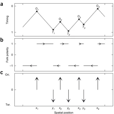
O1 O2 T2 T1 O3 O4 T3 1 Timingb
0 Fork polarity 1 –1c
x1 y1 x2 y2 x3 y3 x4 0 Ori. Ter. Spatial positionFigure 1 | Modeling the spatio-temporal replication program in a single
cell. (a–c) Schematic representations of DNA replication timing r(x) from the
beginning (represented by the value 0 in the y axis) to the end (represented by the value 1 in the y axis) of the S phase (a), replication fork polarity p(x) (b) and spatial location of replication origins (Ori., upward arrows)
and termination sites (Ter., downward arrows) as a function of the spatial position x along the DNA (c). Oi represents the replication origin i located
at xi and firing at time ti. A replication fork proceeding from Oi meets the replication fork coming from Oi + 1 at the termination site Ti, with space-time coordinates yi and ui given in equation (1). Note that one can deduce the fork polarity in b and the origin and termination site location in c by simply
taking successive derivatives of the timing profile in a (equations (3) and (4)).
The fundamental hypothesis at the base of these representations is that the replication fork velocity v is constant.
MaterIals
EQUIPMENT
A computer running Unix/Linux or Mac OSX with access to the Internet crItIcal Windows users should refer to the relevant comments in Equipment Setup.
DNA replication timing profile data formatted as a column text file, in which a value of –1 is imposed for missing data points crItIcal Other data file formats can be used, but the PROCEDURE detailed below must be modified accordingly (see the TROUBLESHOOTING section). Branch of the LastWave signal-processing command language (freely available from our group (B.A.)). As compared with the main branch of the program, this branch implements the color-coding of WTs on the basis of the signed •
•
•
value of the wavelet coefficients and a new fast convolution library based on FFTW (http://www.fftw.org/), a C subroutine library for computing the discrete Fourier transform crItIcal LastWave is open-source software written in C. The version of this program we provide includes a sample data set of the timing profile of chromosome 1 in HeLa cells35,37. The necessary scripts
written in the LastWave command language to perform the protocols are also included. Users who are interested in knowing exactly what is being computed should look into these script files to see how the algorithms are implemented in terms of LastWave commands. Moreover, the numerical implementation of the signal processing tools (WT, convolution and so on) is also available in the
C code. We recommend that interested users read the LastWave C-Application Programming Interface (API) documentation and to contact the corres-ponding author (B.A.) to be directed to the most relevant part of the code.
EQUIPMENT SETUP
LastWave installation To install the branch of LastWave that our group
makes available, follow the instructions at http://perso.ens-lyon.fr/benjamin.
audit/LastWave/. Installation has two dependencies: FFTW3 and X11. crItIcal For Unix/Linux-based systems and Mac OSX, the installation has been extensively tested and should be straightforward. Windows users can use LastWave through CYGWIN, a Linux-like environment for Windows. Note, however, that we have not tested our branch of LastWave and its dependencies on FFTW3 on this platform.
proceDure Getting started
1| Find the shortcut routines written in the LastWave script language in the file replication_timing/rep_timing.
mlw in the LastWave script directory, which can be found in the list variable_scriptDirectory.
nice _scriptDirectory
source replication_timing/rep_timing.mlw
crItIcal step The commands described in this step and in all that follow have to be typed within the LastWave terminal window.
loading the timing profile
2| Change the working directory to the directory in which the data file is stored. As an example, in this protocol, the HeLa
cell timing profile of chromosome 1 determined in a 100-kb-wide window that slides along from the start of the chromosome by incremental steps of 10 kb (the sampling period is thus 10 kb) is uploaded37. The name of the one-column text file that
contains these data is chr1_timing_HeLa_w100kbp_skip10kbp.dat, which can be found in replication_
timing/data.
file cd _scriptDirectory[0] + “/replication_timing/data”
3| Upload the timing profile from a column text file into LastWave. Provide the name of the data file, as well as the
coordinate of the first point and the distance between data points, to the loading routine; for example, for the data file
provided, use 0.05 0.01 to have spatial axis expressed in Mb units. Note that the loading routine assumes that timing
values for windows in which timing cannot be measured are set to − 1.
{rep_timing masked_regions masked_sig} = [load_timing_data “chr1_timing_HeLa_w100kbp_
skip10kbp.dat” 0.05 0.01]
The routine returns a list containing three elements: the timing profile signal (rep_timing), in which missing data have
been linearly interpolated; a binary signal (masked_sig) that is set to 1 in data-less regions and to 0 outside of them;
and a list of signals of size 2 (masked_regions) corresponding to the start and end points of each of these data-less
regions. The variables masked_sig and masked_regions keep track of the regions with missing data. Ensure that
things look as expected by using the command disp to display the timing profile and the binary signal. disp rep_timing masked_sig
?trouBlesHootInG
computing the spatial derivatives at finite resolution using Wt 4| Create two new WT variables named w_N1 and w_N2.
w_N1 = [new &wtrans]
w_N2 = [new &wtrans]
5| Copy the replication timing profile for the mentioned chromosome 1 of HeLa cells as the signal to be analyzed.
w_N1.A[0,0] = rep_timing
w_N2.A[0,0] = rep_timing
6| Compute the WT using the first and second derivatives of the Gaussian function as the analyzing wavelets with a
amin = 5.0;; noct = 6;; nvoice = 10
fftw_cwtd w_N1 amin noct nvoice ‘N1’ − e − 2
fftw_cwtd w_N2 amin noct nvoice ‘N2’ − e − 3
The researcher will obtain the WT described by equation (7) for the series of scales a a= min2(o− +1) v n/ voice, where 1≤o ≤noct
and 0≤v ≤nvoice − 1 (o and v can only have integer values). Scales are expressed in sampling period unit (see Step 2).
These results are stored in the D array of the WT variable w.D[o,v] and can be used as a regular signal (try disp
w_N1.D[4,2]; see the LastWave manual). As amin = 5.0, and the sampling period is 10 kb, when the scale assumes its
minimum value the smoothing Gaussian has a standard deviation of 50 kb. As amax = 5.0×2(6 − 1) + 9/10≈299, when the scale
assumes its maximum possible value the smoothing Gaussian has a standard deviation of 2.99 Mb. Option -e enables to
specify the normalization exponent α of the WT (equation (7)); in order to obtain the first and second derivatives of the smoothed replication timing profile, according to equation (8), α is set to − 2 and − 3, respectively.
crItIcal step Beware that the actual meaning of a specific value for scale a is relative to the definition of the analyzing wavelet. The distance between the two extrema of N(1)(x) is 2 (indeed N( )2( )x 1 (x2 ) x2 2/
2 1
= − −
p e is null at x = ±1). Thus,
the WT with Na( )1 captures the fluctuation of the analyzed profile over a distance 2a. Hence, 2amin = 100 kb is the smallest
meaningful scale for a replication timing profile estimated in a 100-kb sliding window.
7| Correct the slope to be in the usual min and kb units. Note that the units of the output depend on the choice of the
sampling period as the scale unit. Here the timing data are in h, and hence the slopes are expressed in h per 10 kb and the curvature in h per (10 kb)2.
w_N1 = [wtrans_combine {w_N1} %{l}‘return 60*l[0]/10’]
8| Display the results obtained so far. Note that when plotting a WT the scale unit is the scale index ia = nvoice(o − 1) + v
(ia∈[0, 1, …, noct × nvoice − 1]).
disp rep_timing w_N1 w_N2 -..* -norm ‘signedglobal’
9| Explore specific regions of the display of the timing profile and of the space-scale representation of its first and second
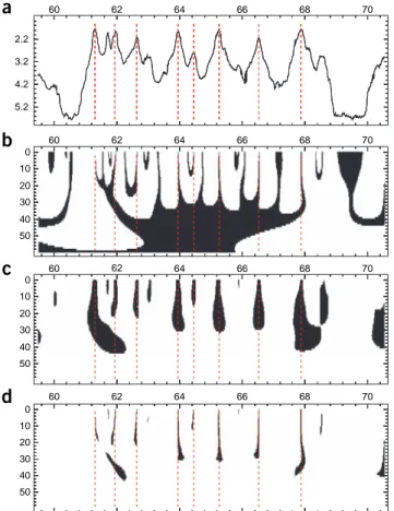
derivatives obtained in Step 8 using the mouse buttons (see LastWave manual for a description of the different zooming modes). As illustrated in Figure 2, when smoothing the timing profile over large distances (large values of scale a), both its
first and second derivatives (equation (8)) appear black (null values of the derivatives), as the signature that the average fork polarity (equation (5)) and the difference between replication origin and termination site densities (equation (6)) are null. At small scale, red (positive values) and blue (negative values) regions are visible; these regions correspond to areas of positive and negative average fork polarity and to areas with either a density of replication origins larger than the density of termination sites or the opposite, respectively (Fig. 2).
?trouBlesHootInG
exploring the apparent speed of replication in space scale
10| Compute an apparent replication speed map introducing the two thresholds for |T( )( ) | N 1
2
− : 0.1 min kb − 1 and 0.5 min kb − 1
(corresponding to an apparent replication speed of 10 kb min − 1 and 2 kb min − 1, respectively).
app_speed = [wtrans_combine {w_N1} %{l}‘return (abs(l[0]) < 0.1) + (abs(l[0]) < 0.5)’]
disp app_speed -..1 -norm ‘global’ -cm ‘color’
The resulting space-scale map (Fig. 2d) presents three types of regions: at small scales, very few black regions are present;
by definition, these are regions in which the timing profile space derivative is > 0.5 (these regions are given a value of 0 in the map), which corresponds to an apparent speed under 2 kb min − 1. Green regions (areas given a value of 1 in the map)
correspond to an apparent speed between 2 kb min − 1 and 10 kb min − 1. Red regions (areas given a value of 2 in the map)
correspond to an apparent replication speed over 10 kb min − 1. Single fork speed estimates in higher eukaryotes are of the
order of 1 kb min − 1 (refs. 37,85,86), which suggests that, for the timing profile analyzed here, only very few regions of
size > 100 kb are replicated systematically by a single fork37 (ANTICIPATED RESULTS).
crItIcal step If one assumes that, regardless of the individual cell taken into account, a specified DNA region R is
and the derivative of the timing profile within the men-tioned R region (equation (5)) is an estimate of the inverse of the fork speed. This assumption leads to define the inverse of d
x r x x
d 〈( )〉Cells,∆ as the local apparent speed of
replication, that is, the speed of a single fork that would result in the same local slope of the timing profile. As the timing profile has a null derivative—an infinite apparent replication speed—in many loci, instead of taking the inverse of the WT obtained with N(1), one can define
space-scale regions belonging to different speed categories; for instance, |T( )( ) | .
N 1 2 0 1
− < min kb − 1 corresponds to regions in
which the apparent replication speed is higher than 10 kb min − 1.
Multiscale detection of peaks in replication timing profiles
11| Intuitively, loci containing very efficient replication origins are expected to appear as local peaks (pointing toward
early timing) of the timing profile34,35. To detect effectively the local peaks alluded to in a noisy timing profile 〈r(x)〉 Cells,∆x,
identify points along the profile that present a null derivative (d
dx〈r x( )〉Cells,∆x∼0) and a strong, positive curvature
(d
x r x x
2
2 0
d 〈( )〉Cells,∆ ), as it is expected at the tip of a peak symmetrical about a vertical axis. As expected for regions that
contain a replication origin, such loci indeed correspond to regions with null average fork polarity (equation (5)) and a higher value for the replication origin density than for the termination site density (equation (6)).
crItIcal step In mathematics and signal processing, graphs are habitually orientated in such a way that Y values
increase upward. According to this convention, loci containing strong replication origins would be expected to appear as downward-pointing peaks, that is, loci with a positive local curvature. To follow instead the common practice in biology, here we choose to display the replication timing axis from the top to the bottom (early S phase at the top of the graph).
This objective is achieved by setting the value of gclass.FramedView.default.reverse to ‘none’ in the file
replication_timing/rep_timing.mlw.
12| Compute the WT with N(1) and scale normalization exponent α = − 1.5, and extract the space-scale regions where d
dx〈r x( )〉Cells,∆x∼0 with the following thresholding TN( ) ( / ) .
13 2 0 02 − < .
w_N1.A[0,0] = rep_timing
fftw_cwtd w_N1 5.0 6 10 ‘N1’ -e -1.5
isflat = [wtrans_combine {w_N1} %{l}‘return abs(l[0]) < 0.02’]
Note that when the profile f being analyzed is the graph of a Brownian motion87, that is, the increments of f are mutually
independent, identically distributed Gaussian variables, then the WT Ty( )0 at scale a is Gaussian with a standard deviation proportional to a3/2. Hence, it is convenient to work with WTs computed with a scale normalization exponent α = − 3/2,
such that the fluctuations of the WT due to the noisy background are independent of the scale of analysis.
2.2 3.2 4.2 5.2 0 60 62 64 66 68 70 60
a
b
c
d
62 64 66 68 70 10 20 30 40 50 0 60 62 64 66 68 70 10 20 30 40 50 0 60 62 64 66 68 70 10 20 30 40 50 Figure 2 | Multiscale decomposition of the DNA replication timing profile inHeLa cells of a fragment of chromosome 1. Figure obtained after conducting Step 10 of the PROCEDURE using the command disp rep_timing w_N1 w_N2 app_speed - ..\[23\] -norm ‘signedglobal’ -..4 -norm ‘global’ -cm ‘color’ -..fv1 -bound 59.5 70.5 ‘*’ ‘*’ and saving the resulting output image as a postscript file using msge Window1 drawps “fig2.ps”. (a) Replication timing expressed in hours since the start of S phase versus the spatial position x along the chromosome. (b) Space-scale representation of the first derivative of the
replication timing profile. (c) Space-scale representation of the second
derivative of the replication timing profile. (d) Three-color map of apparent
replication speed. Note that according to the choice of the first point coordinate and the sampling period in Step 3, in the x axis are reported chromosome coordinates in Mb units. For the color-coding in b and c, see
13| Perform the same computation with wavelet N(2) and extract the space-scale regions where d
x r x x
2
2 0
d 〈( )〉Cells,∆ imposing
the following threshold, T N( ) ( / ) . 23 2 0 06 − > . w_N2.A[0,0] = rep_timing fftw_cwtd w_N2 5.0 6 10 ‘N2’ -e -1.5
iscurved = [wtrans_combine {w_N2} %{l}‘return l[0] > 0.06’]
14| Delineate candidate timing profile peaks as space-scale regions in which the first derivative of the smoothed timing profile
is equal to zero, as determined in Step 12, and the second derivative has a value above the threshold imposed in Step 13.
peaks = [wtrans_combine {isflat iscurved} %{l}‘return l[0]&&l[1]’]
15| Display the results of Steps 12–14 according to the example reported in Figure 3 and explore different regions of the
profile using the mouse buttons. It is apparent in Figure 3d that connected areas of space-scale regions determined in
Step 15, which present a large vertical extension up to small scales, highlight the existence of well-defined peaks in the timing profile. This vertical extension guarantees the robustness of the detection of the underlying putative replication origins with respect to the scale of observation.
?trouBlesHootInG
Identifying u-shaped domains along replication timing profiles
16| If early replicating regions often correspond to peaks in the timing profile, the situation is different in late-replicating
regions in which the profile frequently presents an approximately parabolic shape. In fact, a local U-shaped profile bordered by early replicating regions is a recurrent motif in replication timing profiles, which defines replication U-domains along the genome62. To systematically identify these domains, look for regions in the timing profile that are bordered by points that
are local maxima of the curvature (corresponding to the location in which the U-shape breaks) and that have substantial negative curvature in their central regions, which is the hallmark of a parabolic curve. Note that in these U-domains, the derivative of the replication timing profile has an N-like shape, which indicates the existence of a gradient of replication fork polarity62, a characteristic previously recognized for the germ line in the skew profiles along the human chromosomes52,53,56–58.
17| Compute the WT of the replication timing profile with N(2) and the scale normalization exponent α = −1. Use the
command extrema to compute the extrema representation
associated with this WT (at each scale, the maxima of the modulus of the WT are computed and stored in an extrema
representation variable w_N2.extrep; see LastWave
documentation and online help: help extrema).
w_N2.A[0,0] = rep_timing 2.2
a
b
c
d
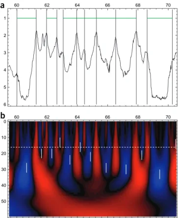
3.2 4.2 5.2 0 60 62 64 66 68 70 60 62 64 66 68 70 10 20 30 40 50 0 60 62 64 66 68 70 10 20 30 40 50 0 60 62 64 66 68 70 10 20 30 40 50Figure 3 | Multiscale detection of peaks in DNA replication timing profiles.
Figure obtained after conducting Steps 12–14 of the PROCEDURE using the command cminit -100 0 ‘grey’;; disp rep_timing isflat iscurved peaks -..* -norm ‘global’ -cm ‘grey’ -..fv1 -bound 59.5 70.5 ‘*’ ‘*’ and saving the resulting output image as a postscript file using msge Window1 drawps “fig3.ps”. (a) Replication timing profile expressed in hours since the start of S phase
versus the spatial position x along the chromosome. (b) Space-scale
representation of the regions (shown in black) in which the timing profile is flat (i.e., TN( )(−13 2/ ) < 0.02). (c) Space-scale representation of the regions (shown in black) in which the timing profile presents a significant positive curvature (i.e., TN( )(−23 2/ ) > 0.06). (d) Regions in which overlapping black-colored regions from b and c define the possible presence of timing peaks.
Vertical red dashed lines have been added to illustrate the locations of the detected putative replication origins59. The x axes indicate reported
fftw_cwtd w_N2 5.0 6 10 ‘N2’ -e -1 extrema w_N2 -i
18| Display the results using the following command.
disp w_N2 w_N2.extrep -..1 -norm ‘signedglobal’
crItIcal step The convenient normalization exponent α of the WT (equation (7)) to estimate the threshold in the central
curvature c depends on the characteristics of the U-shaped timing motif. If the depth of the U-shaped region is proportional to its width (i.e., the value of the depth is proportional to x2 / L, where L is half the width), then c is proportional to 1 / L.
If the depth of the U-shaped region is constant (i.e., its value is proportional to x2 / L2), then c is proportional to 1 / L2. For
a parabolically shaped profile of width 2L, the scale where extreme curvature is observed using the WT is proportional to L. Thus, in order to apply a constant threshold at each scale, in the first scenario a normalization exponent α = − 2 should be used, whereas in the second scenario, the exponent should be α = −1. In this protocol, we emphasize the detection of the largest U-domains, the depth of which is constrained by the duration of the S phase. We therefore choose to represent our data according to the second scenario, which is more permissive than the first for the detection of large U-shaped regions.
19| Extract the set of maxima corresponding to scale 150 kb (a = 15.0) by computing the corresponding octave (o) and
voice (v) numbers, creating a new signal (border_candidates) to hold the list and copying from the extrema
represen-tation (w_N2.extrep) to the new signal the maxima spatial locations (x values) and their WT values (y values).
{o v} = [scale_to_ov_4u 15.0 w_N2.amin w_N2.nvoice]
border_candidates = [new &signal]
extlistosig w_N2.extrep.D[o,v] border_candidates
20| Retain only the maxima locations with a WT value T N( )
( ) . 21 0 15
− ≥ (find the index of interest using find, and then extract
the corresponding subsignal). Display the results obtained so far.
border_candidates = border_candidates[find(border_candidates > = 0.15)]
disp rep_timing border_candidates -S 1 -..2 -curve ‘o’ -3
21| Validate or reject as U-shaped regions areas encompassed between two successive border candidates on the basis of the
value of the curvature of the timing profile at the areas’ mid-point (Fig. 4). Consider as acceptable any region of length 2L
that presents value of TN( )( )−21≤ −0.3 at some scale between 0.24 × 2L and 0.36 × 2L. Indeed, for a parabolically shaped profile
of finite width 2L, the scale at which extreme curvature is observed using T N( )
( ) 21
− is proportional to L, but it also depends on
the shape of the profile at the border of the regions. We have estimated numerically the scale range specified earlier so that its bounds correspond to situations in which both regions flanking the U-shaped domain are either U-domains themselves (then the extreme value of T
N( ) ( ) 21
− is observed at scale 0.24 × 2L) or flat timing profile regions (then the extreme value of T N( )
( ) 21 −
is observed at scale 0.36 × 2L). The script procedure detect_udom recapitulates all these operations; we refer the reader
to the procedure definition and associated comments in the file replication_timing/rep_timing.mlw in LastWave
for a detailed description of all the steps involved.
22| Determine the presence and location of U-domains along the replication timing profile and display the results using the
procedure detect_udom.
do_fig = 1
detect_udom rep_timing masked_sig do_fig
crItIcal step When automating the detection of U-domains, it is important to remove from the set of domains identified those that overlap with regions in which timing data are missing. As exemplified in detect_udom, this objective can
be achieved by estimating, at each scale of analysis, the proportion of points with missing data (i.e., by computing the
moving average of signal masked_sig with T
N( ) ( ) 01
− (equation (8)) and rejecting all U-domains in which this proportion is
?trouBlesHootInG
step 3
problem: Error message appears when reading the timing
data file.
possible reason: Incorrect format of timing data file. The
loading procedure provided in Step 3 applies to replication timing data formatted as a one-column text file, in which a value of − 1 is imposed for missing data points.
solution: LastWave can read data in a wide variety of formats so that users can modify the loading procedure definition
in the replication_timing/rep_timing.mlw file in order to comply with their data format. See the commands
‘read’ and ‘listv cread’ for alternate ways to read data.
help listv cread help read
step 9
problem: Misleading color coding of space-scale representations. possible reason: Incorrect color-coding options have been used.
solution: To avoid misinterpretation of space-scale representations, users must be aware of the diverse color-coding options
offered by LastWave. The default color-coding of WT coefficients assigns colors on the basis of WT absolute values, and the transfer function between absolute values and colors are recalculated at each scale. This default color scheme corresponds
to the display option -norm ‘lglobal’. A global transfer function calculated across all the investigated scales between
the WT absolute values and colors is obtained with the display option -norm ‘global’ (see the LastWave documentation
relative to the wtrans1d package). For the purposes of this protocol, a global signed mapping rule has been implemented
that can be accessed with the display option -norm ‘signedglobal’ used above. The reason for this choice is
exemplified by the fact that displaying the derivatives of the smooth timing profile in Step 8 using the default color transfer
function (disp rep_timing w_N1 w_N2) instead of the prescribed signed mapping rule (-..* -norm
‘signed-global’) would produce pictures with high-intensity blue and red colorations at all scales, which would in turn prevent
researchers from making the observation that the amplitude of the derivatives is negligible at large scales (Fig. 2),
as discussed in Step 9.
Note that users have control of the color maps. A color map from blue to red is set as the default color map in the
replication_timing/rep_timing.mlw file using the command colormap current ‘b2r’; an alternative
rainbow color map can be chosen with the display option -cm ‘color’. Color maps can be visualized using cmdisp
‘color’ and cmdisp ‘b2r’.
step 15
problem: When displaying the result of the peak detection protocol as exemplified in Figure 3, the user notices space-scale
patterns that are not coherent across scales and that are in clear contrast with the well-defined vertical structures marked by the red dashed lines in Figure 3.
60 1 2 3 4 5 6 0 10 20 30 40 50 62 64 66 68 70 60 62 64 66 68 70
a
b
Figure 4 | Identifying replication timing U-domains. This image wasobtained after conducting Steps 16–22 of the PROCEDURE using the command disp TheWindow -..fv1 -bound 59.5 70.5 “*” “*” (in order to zoom into the same regions as in Figs. 2 and 3) and after saving the resulting output image as a postscript file with msge TheWindow drawps “fig4.ps”. (a) Replication timing profile expressed in hours since the start of S phase versus the spatial position x along the DNA: black vertical lines mark candidate borders of U-domains detected as the maxima of T
N( )
( ) 21
− at a 15-kb scale. Horizontal green bars are drawn between two successive candidate borders when the region of size 2L was selected as a replication U-domain. (b) Space-scale representation
of the WT T
N( )
( ) 21
− of the timing profile. The horizontal dashed line marks the scale, a = 15 kb. The vertical white segments at the mid-position between two successive candidate borders mark the scale range 0.24 × 2L and 0.36 × 2L over which the minimal value of T
N( )
( ) 21
− is searched. The selected U-domains are such that min T
N( )
( ) 21
− ≤ − 0.3. The x axes show reported chromosome coordinates in Mb units.
possible reason: Wavelet coefficient threshold values are
inadequate with respect to noise level. If the wavelet coefficient threshold values used in Steps 11–15 are too permissive, then the noise-related peaks in replication timing profiles will incorrectly be detected as putative replication origins.
solution: Adjust the threshold values on wavelet coefficients so that they are more stringent (i.e., a smaller threshold value
of the first derivative of the smoothed replication timing profile in Step 12 and a larger value of the second derivative in Step 13). Please note that in the ‘opposite’ scenario, in which the threshold values are too stringent, users will notice that obvious replication timing peaks are missed, resulting in false negatives.
●tIMInG
Computing time and memory space requirements are not a limitation with today’s desktop computers. The complete
procedure, as described above, should not take more than 1 h, and it can be reproduced in tens of minutes by an experienced user. However, in order to become proficient, a new user needs to learn about the general syntax and capabilities of LastWave signal-processing command language. LastWave offers comprehensive documentation (that can be downloaded from the website) and online help for most commands (use help < command name > ), as well as interactive demonstrations; just
type Demo from the LastWave command line and follow the instructions. Learning the basics of the program can take a few
hours, but achieving the proficiency to be able to fully exploit the scripting power of the software and learning how to use the C-API may take days.
antIcIpateD results
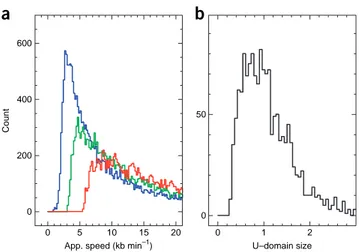
The procedure presented here enables researchers to extract quantitative information that can be used to model the spatio-temporal DNA replication program in multicellular organisms. For instance, the histograms of apparent replication speed values reported in Figure 5a and obtained through this protocol show that, in HeLa cells, practically no regions larger
than 100 kb replicate at a speed lower than 2 kb min − 1 (ref. 37). This scenario corresponds to the quasi-absence of black
regions in Figure 2d. In these cells, the speed of a single replication fork measured using DNA combing was shown to have
a narrow distribution around a mean value of ~0.7 kb min − 1 (ref. 37). Accordingly, the histograms of apparent replication
speed in Figure 5a indicate that in HeLa cells chromosome 1 has no large DNA regions that undergo replication in a strictly
unidirectional manner and that replication timing gradients correspond to a sequential pattern of replication origin activations37. Note that this result holds true for all chromosomes.
Detection of peaks in the replication timing profile achieved as described in Steps 11–15 (Fig. 3) has been applied to
the DNA replication timing profiles of six different human cell types59. Comparison of data on the locations of these
( > 1,000) putative replication origins reveals a substantial degree of conservation of replication origins among cell types. These data also provide further evidence in favor of the putative germ-line replication origins previously identified via the analysis of skew profiles52,53,57,58.
The procedure detailed here for detecting U-shaped motifs in the replication timing profile (Steps 16–22 and Fig. 4)
enabled us to reliably detect megabase-size U-domains (Fig. 5b), which cover about half of the genome in seven human
cell types (from 39.6% in lymphoblastoid cell line TL010 to 61.9% in stem cell line BG02)62. Notably, Hi-C data65 show
that U-domains in the DNA replication timing profile correspond to self-interacting high-order chromatin structural units. Replication U-domains are thus indicators of a segmentation of the genome into independent replication units, and their identification affords insight into the organization of the replication program in the human genome.
600
a
b
400
Count
App. speed (kb min–1)
0 5 10 15 20 U–domain size 0 1 2 200 50 0 0
Figure 5 | Quantitative analysis of replication program parameters.
(a) Histogram of the apparent (App.) speed of replication for the HeLa cell
replication timing profile of chromosome 1 as analyzed in the PROCEDURE; the counts correspond to the number of 100-kb sliding windows within each apparent speed bins computed from horizontal cuts of the WT in Figure 2b
at scales 2a = 100 kb (blue), 2a = 400 kb (green) and 2a = 800 kb (red). (b) Histogram of replication U-domain size values obtained for the complete
human genome with the methodology presented in Steps 16–22 of the PROCEDURE applied to the replication timing profile of HeLa cells62.
acknoWleDGMents We thank all the contributors to the LastWave project and
in particular E. Bacry for the development of the LastWave kernel. This work was supported by the Agence National de la Recherche under projects HUGOREP (ANR PCV 2005) and REFOPOL (ANR BLANC SVSE 6), and by grants from FRM (équipe labélisée), the ARC and the Ligue contre le Cancer (Comité de Paris) to O.H.
autHor contrIButIons All authors contributed equally to the design and
application of the protocols presented in this paper. B.A. and A.A. wrote the paper.
coMpetInG FInancIal Interests The authors declare no competing financial
interests.
Published online at http://www.nature.com/doifinder/10.1038/nprot.2012.145. Reprints and permissions information is available online at http://www.nature. com/reprints/index.html.
1. Bell, S.P. & Dutta, A. DNA replication in eukaryotic cells. Annu. Rev.
Biochem. 71, 333–374 (2002).
2. DePamphilis, M.L. (ed). DNA Replication and Human Disease (Cold Spring Harbor Laboratory Press, 2006).
3. Aladjem, M.I. Replication in context: dynamic regulation of DNA replication patterns in metazoans. Nat. Rev. Genet. 8, 588–600 (2007).
4. Hamlin, J.L., Mesner, L.D. & Dijkwel, P.A. A winding road to origin discovery. Chromosome Res. 18, 45–61 (2010).
5. Mesner, L.D., Crawford, E.L. & Hamlin, J.L. Isolating apparently pure libraries of replication origins from complex genomes. Mol. Cell 21,
719–726 (2006).
6. Lucas, I. et al. High-throughput mapping of origins of replication in human cells. EMBO Rep. 8, 770–777 (2007).
7. The ENCODE Project Consortium. Identification and analysis of functional elements in 1% of the human genome by the ENCODE pilot project.
Nature 447, 799–816 (2007).
8. Cadoret, J.-C. et al. Genome-wide studies highlight indirect links between human replication origins and gene regulation. Proc. Natl. Acad. Sci. USA 105,
15837–15842 (2008).
9. Karnani, N., Taylor, C.M. & Dutta, A. Microarray analysis of DNA replication timing. Methods Mol. Biol. 556, 191–203 (2009).
10. Cayrou, C. et al. Genome-scale analysis of metazoan replication origins reveals their organization in specific but flexible sites defined by conserved features. Genome Res. 21, 1438–1449 (2011).
11. Mesner, L.D. et al. Bubble-chip analysis of human origin distributions demonstrates on a genomic scale significant clustering into zones and significant association with transcription. Genome Res. 21, 377–389 (2011).
12. Hyrien, O. & Méchali, M. Chromosomal replication initiates and terminates at random sequences but at regular intervals in the ribosomal DNA of
Xenopus early embryos. EMBO J. 12, 4511–4520 (1993).
13. Hyrien, O., Maric, C. & Méchali, M. Transition in specification of embryonic metazoan DNA replication origins. Science 270, 994–997 (1995).
14. Gerbi, S.A. & Bielinsky, A.K. DNA replication and chromatin. Curr. Opin.
Genet. Dev. 12, 243–248 (2002).
15. Schübeler, D. et al. Genome-wide DNA replication profile for Drosophila
melanogaster: a link between transcription and replication timing. Nat. Genet. 32, 438–442 (2002).
16. Anglana, M., Apiou, F., Bensimon, A. & Debatisse, M. Dynamics of DNA replication in mammalian somatic cells: nucleotide pool modulates origin choice and interorigin spacing. Cell 114, 385–394 (2003).
17. Fisher, D. & Méchali, M. Vertebrate HoxB gene expression requires DNA replication. EMBO J. 22, 3737–3748 (2003).
18. Gilbert, D.M. Making sense of eukaryotic DNA replication origins.
Science 294, 96–100 (2001).
19. MacAlpine, D.M. & Bell, S.P. A genomic view of eukaryotic DNA replication. Chromosome Res. 13, 309–326 (2005).
20. Méchali, M. Eukaryotic DNA replication origins: many choices for appropriate answers. Nat. Rev. Mol. Cell Biol. 11, 728–738 (2010).
21. Gilbert, D.M. Evaluating genome-scale approaches to eukaryotic DNA replication. Nat. Rev. Genet. 11, 673–684 (2010).
22. Ryba, T., Battaglia, D., Pope, B.D., Hiratani, I. & Gilbert, D.M.
Genome-scale analysis of replication timing: from bench to bioinformatics.
Nat. Protoc. 6, 870–895 (2011).
23. Raghuraman, M.K. et al. Replication dynamics of the yeast genome.
Science 294, 115–121 (2001).
24. MacAlpine, D.M., Rodriguez, H.K. & Bell, S.P. Coordination of replication and transcription along a Drosophila chromosome. Genes Dev. 18,
3094–3105 (2004).
25. Eaton, M.L. et al. Chromatin signatures of the Drosophila replication program. Genome Res. 21, 164–174 (2011).
26. Farkash-Amar, S. et al. Global organization of replication time zones of the mouse genome. Genome Res. 18, 1562–1570 (2008).
27. Hiratani, I. et al. Global reorganization of replication domains during embryonic stem cell differentiation. PLoS Biol. 6, e245 (2008).
28. White, E.J. et al. DNA replication-timing analysis of human chromosome 22 at high resolution and different developmental states. Proc. Natl. Acad.
Sci. USA 101, 17771–17776 (2004).
29. Woodfine, K. et al. Replication timing of the human genome. Hum. Mol.
Genet. 13, 191–202 (2004).
30. Jeon, Y. et al. Temporal profile of replication of human chromosomes.
Proc. Natl. Acad. Sci. USA 102, 6419–6424 (2005).
31. Woodfine, K. et al. Replication timing of human chromosome 6. Cell Cycle 4,
172–176 (2005).
32. Karnani, N., Taylor, C., Malhotra, A. & Dutta, A. Pan-S replication patterns and chromosomal domains defined by genome-tiling arrays of ENCODE genomic areas. Genome Res. 17, 865–876 (2007).
33. Desprat, R. et al. Predictable dynamic program of timing of DNA replication in human cells. Genome Res. 19, 2288–2299 (2009).
34. Hansen, R.S. et al. Sequencing newly replicated DNA reveals widespread plasticity in human replication timing. Proc. Natl. Acad. Sci. USA 107,
139–144 (2010).
35. Chen, C.-L. et al. Impact of replication timing on non-CpG and CpG substitution rates in mammalian genomes. Genome Res. 4, 447–457
(2010).
36. Weddington, N. et al. Replicationdomain: a visualization tool and comparative database for genome-wide replication timing data.
BMC Bioinformatics 9, 530 (2008).
37. Guilbaud, G. et al. Evidence for sequential and increasing activation of replication origins along replication timing gradients in the human genome. PLoS Comput. Biol. 7, e1002322 (2011).
38. Ryba, T. et al. Evolutionarily conserved replication timing profiles predict long-range chromatin interactions and distinguish closely related cell types. Genome Res. 20, 761–770 (2010).
39. Yaffe, E. et al. Comparative analysis of DNA replication timing reveals conserved large-scale chromosomal architecture. PLoS Genet. 6, e1001011
(2010).
40. Friedman, K.L., Brewer, B.J. & Fangman, W.L. Replication profile of
Saccharomyces cerevisiae chromosome VI. Genes Cells 2, 667–678 (1997).
41. Patel, P.K., Arcangioli, B., Baker, S.P., Bensimon, A. & Rhind, N. DNA replication origins fire stochastically in fission yeast. Mol. Biol. Cell 17,
308–316 (2006).
42. Rhind, N. DNA replication timing: random thoughts about origin firing.
Nat. Cell Biol. 8, 1313–1316 (2006).
43. Czajkowsky, D.M., Liu, J., Hamlin, J.L. & Shao, Z. DNA combing reveals intrinsic temporal disorder in the replication of yeast chromosome VI.
J. Mol. Biol. 375, 12–19 (2008).
44. de Moura, A.P.S., Retkute, R., Hawkins, M. & Nieduszynski, C.A. Mathematical modelling of whole chromosome replication. Nucleic Acids
Res. 38, 5623–5633 (2010).
45. Rhind, N., Yang, S.C. & Bechhoefer, J. Reconciling stochastic origin firing with defined replication timing. Chromosome Res. 18, 35–43 (2010).
46. Retkute, R., Nieduszynski, C.A. & de Moura, A. Dynamics of DNA replication in yeast. Phys. Rev. Lett. 107, 068103 (2011).
47. Yang, S.C., Rhind, N. & Bechhoefer, J. Modeling genome-wide replication kinetics reveals a mechanism for regulation of replication timing.
Mol. Syst. Biol. 6, 404 (2010).
48. Hyrien, O. & Goldar, A. Mathematical modelling of eukaryotic DNA replication. Chromosome Res. 18, 147–161 (2010).
49. Goldar, A., Marsolier-Kergoat, M.-C. & Hyrien, O. Universal temporal profile of replication origin activation in eukaryotes. PLoS ONE 4, e5899 (2009).
50. Baker, A., Audit, B., Yang, S.C., Bechhoefer, J. & Arneodo, A. Inferring where and when replication initiates from genome-wide replication timing data. Phys. Rev. Lett. 108, 268101 (2012).
51. Goldar, A., Labit, H., Marheineke, K. & Hyrien, O. A dynamic stochastic model for DNA replication initiation in early embryos. PLoS ONE 3, e2919
(2008).
52. Brodie of Brodie, E.-B. et al. From DNA sequence analysis to modeling replication in the human genome. Phys. Rev. Lett. 94, 248103 (2005).
53. Touchon, M. et al. Replication-associated strand asymmetries in mammalian genomes: toward detection of replication origins. Proc. Natl.
Acad. Sci. USA 102, 9836–9841 (2005).
54. Touchon, M., Nicolay, S., Arneodo, A., d’Aubenton-Carafa, Y. & Thermes, C. Transcription-coupled TA and GC strand asymmetries in the human genome. FEBS Lett. 555, 579–582 (2003).