Coulomb blockade and transfer of electrons one by one

HAL Id: tel-00185219

https://tel.archives-ouvertes.fr/tel-00185219

Submitted on 5 Nov 2007

HAL is a multi-disciplinary open access archive for the deposit and dissemination of sci-entific research documents, whether they are pub-lished or not. The documents may come from teaching and research institutions in France or

L’archive ouverte pluridisciplinaire HAL, est destinée au dépôt et à la diffusion de documents scientifiques de niveau recherche, publiés ou non, émanant des établissements d’enseignement et de recherche français ou étrangers, des laboratoires

Coulomb blockade and transfer of electrons one by one

H. Pothier

To cite this version:

H. Pothier. Coulomb blockade and transfer of electrons one by one. Condensed Matter [cond-mat]. Université Pierre et Marie Curie - Paris VI, 1991. English. �tel-00185219�

THESE DE DOCTORAT DE L'UNIVERSITE PARIS 6 Specialite:

Physique des Solides

presentee par Hugues POTHIER

pour obtenir le titre de DOCTEUR DE L'UNIVERSITE PARIS 6

Sujet de la these:

BLOCAGE DE COULOMB ET TRANSFERT D'ELECTRONS UN PAR UN

Soutenue le 16 septembre 1991 devant le jury compose de MM: J. BOK

C. COHEN-TANNOUDJI M.DEYORET

K. YON KLITZING B. PANNETIER

REMERCIEMENTS

J'ai eu le bonheur de faire ce travail de these dans Ie groupe de " Quantronique" , avec Michel Devoret, Daniel Esteve et Cristian Urbina. Ils m'ont consacre une grande partie de leur temps, et m'ont transmis, outre leur savoir et leur savoir-faire, leur enthousiasme et leur esprit critique. Je les en remercie tres sincerement.

Je remercie Pief Orfila qui, par ses competences techniques et son esprit d'initiative, a ete l'artisan de la reussite des experiences.

Je remercie Emmanuel Turlot d'avoir guide mes premiers pas au laboratoire.

Philippe Lafarge est depuis un an mon compagnon de tournevis, de potentiometre et de clavier. L'experience de la boite it electrons ("single electron box") que je presente ici est aussi en grande partie la sienne. Travailler en sa compagnie m'a ete tres agreable.

Edwin Williams nous a apporte ses connaissances, ses astuces et son acharnement lors de cette meme experience. Je l'en remercie.

La partie theorique de cette these doit beaucoup it la collaboration avec Hermann Grabert et Gert Ingold de l'Universite d'Essen.

La collaboration avec Valerie Anderegg, Bart Geerligs et Hans Mooij a ete Ie veritable point de depart de nos experiences. L'experience du "turnstile" est le resultat le plus tangible de cette collaboration. Mais ils nous ont aussi appris it fabriquer des echantillonsj en nous communiquant regulierement leurs resultats, et grace a de nombreuses discussions, ils ont eu une tres large part it ce travail.

En plus des competences scientifiques, je tiens egalement it remercier Morvan Salez qui, pendant l'annee qu'il a passe dans le groupe de Quantronique, y a fait regner une atmosphere constante de bonne humeur.

Je remercie Pierre Berge de m'avoir accueilli dans le Service de Physique du Solide et de Resonance Magnetique, et Daniel Beysens pour m'avoir permis de continuer ce travail au sein du Service de Physique de l'Etat Condense. Parmi les physiciens que j'y ai cottoye et avec qui j'ai eu l'occasion de discuter, je tiens it remercier plus particulierement Christian Glattli et Marc Sanquer.

de visiter plusieurs laboratoires. Chaque discussion, chaque visite m'a un peu plus ouvert les yeux. Je tiens

a

remercier plus particulierement Dima Averin, Per Delsing, Klaus von Klitzing, John Martinis, Yuri Nazarov, Jurgen Niemeyer et Stefan Verbrugh.

Lors de la redaction de cette these, j'ai beneficie des remarques et des conseils fournis de Michel Devoret, Daniel Esteve, Cristian Urbina et Hermann Grabert. Andrew Cleland a bien voulu en plus rectifier mon anglais parfois (souvent?) approximatif. Madame Gaujour a mis son talent dans plusieurs des dessins qui illustrent cette these. Je les en remercie vivement.

Mon frere aine Jacques a eu l'idee de comparer Ie fonctionnement de notre premier cir-cuit transferant les electrons un par un avec un de ces tourniquets auxquels les utilisateurs du metro parisien (ou New-Yorkais) sont habitues. Merci done au parrain du "turnstile"!

Je remercie particulierement Julien Bok, Claude Cohen-Tannoudji, Klaus von Klitzing et Bernard Pannetier d'avoir accepte de faire partie du jury de rna these. Leur temps est precieux, et j'apprecie d'autant plus l'interet et l'attention qu'ils ont bien voulu porter

a

mon travail.

Enfin, je suis tres reconnaissant envers tous ceux qui m'ont montre que leurs talents de physicien n'excluaient pas leur interet pour I'archeologie, l'architecture, la peinture, les enfants ou la clarinette.

TABLE OF CONTENTS

1. INTRODUCTION . . . 1

ORGANIZATION OF THIS WORK 4

2. LOCAL VERSUS GLOBAL RULES:

EFFECT OF THE ELECTROMAGNETIC ENVIRONMENT

ON THE TUNNELING RATE OF A SMALL TUNNEL JUNCTION . . . , 6 2.1. DESCRIPTION OF THE DEGREES OF FREEDOM OF THE CIRCUIT 7 2.1.1. Description of the tunnel junction . . . 9

2.1.2. The low-pass and high-pass environments 9

2.1.3. The electromagnetic environment of the pure tunnel element 11

2.2. LOW PASS ENVIRONMENT 14

2.2.1. The hamiltonian of the circuit . . . 14

2.2.2. Tunneling rate calculation . . . 18 2.2.2.1. The basic calculation: one junction in series with an

inductance at zero temperature . . . 18 2.2.2.2. General calculation at zero temperature . . 22 2.2.2.3. Application to a purely resistive environment . 28 2.2.2.4. Calculation at finite temperature . . . 30 2.2.3. Observability of the Coulomb blockade of tunneling on a

junction in a low-pass electromagnetic environment . 31

2.3. HIGH-PASS ENVIRONMENT . . 32

2.3.1. Hamitonian of the circuit . 32

2.3.2. Calculation of the rate . . . 32 2.3.3. Observability of the Coulomb blockade of tunneling in a high-pass

environment . . . 35

2.3.3.1. Very low impedance . . 35

2.3.3.2. Very high impedance . 37

2.4. CONCLUSION . . . 39 3. EXPERIMENTAL TECHNIQUES . 40 3.1. FABRICATION OF JUNCTIONS . 40 3.1.1. Wafer preparation. . . 42 3.1.2. Electron-beam patterning . 43 3.1.3. Development. Etching . . . 45

3.1.4. Evaporation of aluminium. Lift-off . 46

3.2. DESIGN OF DEVICES . . . 46

3.2.1. Calculation of planar capacitances . . 46

3.2.2. Simulation of small junction circuits . 50

3.3. MEASUREMENT TECHNIQUES. . . 51

"SINGLE ELECTRON BOX" . 55

4.1. THERMAL EQUILIBRIUM AVERAGES . 55

4.2. THE SET TRANSISTOR . . . 60

4.2.1. Device description. . . 60

4.2.2. Experimental determination of the parameters of the SET transistor and performances as an electrometer . . . 62 4.3. DETAILED OBSERVATION AND CONTROL OF THE COULOMB

BLOCKADE OF TUNNELING IN THE ELECTRON BOX . 64

5. CONTROLLED TRANSFER OF SINGLE CHARGES 74

5.1. THE TURNSTILE . . . 76

5.1.1. Operation principle . . . 76

5.1.2. Controlled transfer of single electrons one by one in

2+2 junction turnstiles . . . 82

5.1.3. Deviations from the ideal 1=ef behaviour. . 84

5.1.3.1. Effect of the temperature . 86

5.1.3.2. Effect of the operation frequency . 86

5.1.3.3. Hot electron effects . 88

5.1.3.4. Effect of co-tunneling . . . 90

5.2. THE PUMP . . . 92

5.2.1. Controlled transfer of electrons one by one in a 3-junction pump . 92 5.2.2. Operation principle of the N-pump . . . 103 5.2.3. Deviations from the regular transfer of single charges . . . 105 5.2.3.1. Co-tunneling effects in the 3-junction pump . . . 105 5.2.3.2. Frequency dependence of the current at zero bias voltage 105 5.2.3.3. Hot electron effects in the N-junction pump 108 5.2.3.4. Co-tunneling rates in the N-pump operation 109

5.3. SINGLE ELECTRON DEVICES AND METROLOGY 114

5.3.1. Transferring electrons one by one: what for? 114

5.3.2. Is metrological accuracy achievable? 116

5.3.3. Conclusion . . . 117

6. CONCLUDING SUMMARY. 119

APPENDIX 1. THE INCOHERENT COOPER PAIR TUNNELING RATE 122

APPENDIX 2. PUMP PATTERN FILE FOR THE SEM . . . 124

APPENDIX 3. CO-TUNNELING. . . 126

A3.1. CO-TUNNELING RATE THROUGH TWO JUNCTIONS IN SERIES 126

A3.2. CO-TUNNELING RATE THROUGH A LINEAR ARRAY 129

APPENDIX 4. PAPER 1 134

APPENDIX 5. PAPER 2 148

1. INTRODUCTION

Striking photographs of artificial arrangements of a few xenon atoms (Eigler and Schweizer, 1990) and studies of single Rydberg atoms (Goy et al.,1983) recently illustrated the ability of physicists to deal with individual elementary constituents of matter. The trapping of single electrons with electronic and magnetic fields (Van Dyck et al., 1986) had demonstrated before that electrons could also be isolated in vaccuum chambers. In the present work, single electrons are manipulated one by one in the solid state. The metallic circuits we have fabricated are the first genuine" electronic" devices, in the sense that they deal with single electrons at the macroscopic level. They are based on the combination of two well-known ingredients: the quantum tunneling effect and classical electrostatics. Spectacular consequences of such a combination were predicted in 1984 and 1986 (Zorin and Likharev, 1984; Averin and Likharev, 1986): firstly, the tunneling of electrons through a small-capacitance tunnel junction should be suppressed at low temperatures and low voltages because tunneling of a single electron would increase by too large an amount the electrostatic energy of the junction. These authors called this effect the Coulomb blockade of tunneling. Secondly, they predicted the existence of voltage oscillations across a current biased small-capacitance junction. Despite substantial experimental efforts, the Coulomb blockade of tunneling had never been clearly observed in circuits containing only one junction before our work. The reason for this failure is that, in practice, the biasing circuit cannot be made perfect enough to forbid quantum fluctuations of the junction capacitor charge larger than the electron charge e. The starting point of our work is a thorough understanding of how these fluctuations suppress the Coulomb blockade. From this understanding a different approach of the problem emerged. The key concept lies in the fact that the charge on an isolated piece of metal (" island") must correspond to an integer number of electron charges. This quantization of the macroscopic charge results in the quenching of the charge fluctuations and thus leads to Coulomb blockade.

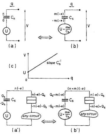
To see this, let us start from the beginning and examine what happens when a battery charges a capacitor. The charge

Q

on the surface of the metal electrodes of the capacitor arises from the very small displacement of the electrons with respect to the fixed metal ions.

The variable Q is therefore continuous, and is not constrained to be an integer number of elementary charges e. However, if one opens a switch placed between the capacitor and the battery, a metallic island is created. Just as an isolated ion carries a well defined number of electrons, the charge of this island, disconnected from any charge reservoir, corresponds to an integer number of electrons which remains constant. An intermediate situation is achieved when the switch is replaced by a tunnel junction (see Fig. 1.1) with high tunnel resistanceRT. We have called this circuit a "single electron box" (see Fig. 1.2). Inthe single electron box, electrons are able to tunnel in and out of the island through the junction. The charge which tunnels through the junction can only be an integer number of electron charges. The instantaneous charge of the island, in units of e, is thus constrained to be an integer number n. IT one wishes to control this number, its thermal fluctuations

have to be suppressed. This is achieved by lowering the temperature until the typical energy kBT of the fluctuations is much lower than the energy e2/2(C

+

Cs) required to charge the island with one electron (C and C

s

are the capacitances of the junction and of the capacitor, respectively). Under this condition, the number of electrons in the island will anchor itself to the integer nmin which minimizes the electrostatic energy of the whole circuit. In fact, in addition to being subject to thermally induced fluctuations,

n is also subject to quantum fluctuations. However, these fluctuations are negligible if RT ~ RK, where RK

=

hi

e2 ~ 25.8 kO is the resistance quantum. In practice, the conditions needed to observe the anchoring phenomenon can be achieved by fabricating circuits with tunnel junctions withRT ~ 100 kO and areas of the order of (100 nm)2, which results in capacitances below 1fF. The capacitanceC

s

can be made smaller than 1fF by designing a micron size island and avoiding large metallic islands in the neighbourhood. With capacitances of this magnitude, the condition e2/2(C

+

Cs) ~ kBT is satisfied at dilution refrigerator temperatures (T ~ 50 mK).

(a)

(b)

Fig. 1.1 (a) Tunnel Junction: a tunnel Junction consists of two pieces of metal separated by a thin insulating layer. This insulator is a tunnel barrier for electrons. The current

I(t)

through such a tunnel Junction is proportional to the voltage applied to it (provided the voltage is much lower than the Fermi energies of the metals). The ratio between the voltage and the current defines the "tunnel resistance" R_T of the Junction. It is generally believed (A verin andLikharev, 1986) that zf RT is much larger that the quantum of resistance R_K = hie2 ::::25.8 kf],the electrons are localized on either side of the junction tunnel barrier. The electrons tunnel through the barrier as separate entities, and this quantum mechanical process occurs in less than10-15 s. The current through such a tunnel Junction as a function of time (b) is then composed of peaks of area e, each one corresponding to the tunneling of a single electron through the tunnel barrier (Fig. 1.1). The time between peaks is a random variable whose average value determines the value of the current. The current noise resulting from this Poisson process is called shot noise; its spectrum at low enough temperature (kBT ~ eRTI) is given by B[(w) = eI. While this spectrum was measured as early as 1922, the individual peaks have never been observed.

n

Fig. 1.2 Single electron box. This basic circuit contains a metallic "island", which is the electrode between the dielectric of the capacitor and the

insulat-ing layer of the junction. The number n of extra electrons on the island is

controlled by a voltage source U. The island capacitance is the sum of the

junction capacitance C and of the capacitance Cgo RT is the junction tunnel

resistance.

ORGANIZATION OF THIS WORK

In chapter 2, we examine how the circuit connected to a small-capacitance tunnel junction influences the tunneling rate of electrons. We show that the tunneling through one junction can be blocked only if the junction is placed in an environment with a high impedance, such as the one provided by i) a small capacitor,

ii)

another small junction or

iii)

a very large ohmic resistance (compared to RK). We show that the simplest way to observe Coulomb blockade of tunneling is in circuits containing a metallic island, such as the electron box and, more generally, in circuits with several junctions connected in series. The case of a large resistor is the most difficult to implement experimentally (Cleland

et

al., 1990).

The experimental setup, including our filtering and measurement techniques, is pre-sented in chapter 3, together with the computer programs we have used to calculate planar capacitances and to simulate the behaviour of one-dimensional arrays of junctions. We also describe the nanolithography techniques that we used to fabricate the devices.

We describe in chapter 4 the experiment on the electron box, which is the first device containing only one junction to display the Coulomb blockade of tunneling. Furthermore, in this device, we controlled the charge of an island at the level of the single electron charge by applying a capacitively-coupled gate voltage.

At this point, the question naturally arises whether one can also control a current elec-tron by elecelec-tron. We have designed and operated two devices which achieve this controlled transfer: the" turnstile" and the "pump". Here the transfer is clocked by external signals applied to gates. This is the central subject of chapter 5. At the end of this chapter, appli-cations of pumps and turnstiles to metrology are discussed: circuits manipulating charges in the quantum limit are candidates for a new representation of the ampere, in the same way as Josephson junction arrays provide a representation of the volt and quantum Hall samples a representation of the ohm. The limits in precision of present day single-electron devices are discussed: the most serious source of error to the regular transfer of single electrons is the possibility of simultaneous tunneling through several junctions. This is discussed in appendix 3.

Two papers are included in appendices 4 and 5. Paper 1 (ref. Devoret et al., 1990a) deals with the influence of the electromagnetic environment on the tunneling rate through a tunnel junction. Itgives the extension of the calculation of chapter 2 to finite temperatures. The results of paper 1 were developed in later publications (Devoret et al., 1990bj Grabert

et

al., 1991a&b). Paper 2 describes the first device with which we transferred electrons one by one: a "turnstile", that we operated in collaboration with Geerligs, Anderegg, Holweg and Mooij of T.U. Delft (Geerligs

et

al., 1990a). This complements chapter 5, where the experimental results were obtained using a different sample. The turnstile and the pump have also been discussed in other publications (Anderegg

et

al., 1990; Devoret

et

al., 1991j Pothier

et

al., 1991a&bj Urbina

et

al., 1991a&b).

2. LOCAL VERSUS GLOBAL RULES:

EFFECT OF THE ELECTROMAGNETIC ENVIRONMENT ON THE TUNNELING RATE OF A SMALL TUNNEL JUNCTION

The environment of a tunnel junction determines the Coulomb blockade of tunneling through it. The understanding of the role of the environment is essential for the design of circuits using the Coulomb blockade of tunneling and for the simulation of their behaviour. The calculations of this chapter show that the tunnel rates in the circuit we designed are given by a simple expression, known as the" global rule". They are used in the SETCAD program presented in section 2.2.2 and are the basis for the chapters4 and 5.

Historically, the Coulomb blockade of tunneling through a tunnel junction placed in a circuit was described using two simplified approaches. The first one was to assume that, since tunneling occurs fast, only the part of the circuit which is very close to the junction determines the blockade (Likharev and Zorin, 1985): the rest of the circuit" does not have time" to be involved. The radius around the junction which participates was called the "electromagnetic horizon". This radius was thought by some to be determined by the speed of light and the traversal time of tunneling (Biittiker and Landauer, 1986). For others, it was thought to be the distance associated with a "quantum time" hi t1E, where

t1E is the thermal energy kBT or eV (Delsing et al., 1989; Nazarov, 1989). Whatever it may be, a local energy change of the system therefore determines the blockade: this gives the local rule (Geigenmiiller and Schon, 1989). The second way is to consider the junction and the circuit as a whole coherent unit, and the blockade of tunneling through the junction depends on the energy change of the whole circuit when one electron tunnels: this is the global rule (Geigenmiiller and Schon, 1989; Likharev et al., 1989).

Cleland

et

al. (1990) first approached the solution of the problem by considering the quantum fluctuations of the junction capacitor charge due to the electromagnetic environment of the junction. Using a semiclassical picture of tunneling across a junction whose capacitor charge is fluctuating, they found that Coulomb blockade only occurs when the quantum fluctuations of the junction charge are much less than one electron charge.

connected to an environment of impedance

Z(w)

in the limit ofzero traversal time (the case of finite traversal time, which is relevant in semiconductor circuits with Schottky barriers, has been considered by Nazarov (1991)). We treat the environment and the electronic degrees of freedom quantum mechanically, and use the Fermi Golden rule to compute the probability that an electron tunnels and induces an excitation of the environment. These inelastic tunneling channels are the dominant ones only if the fluctuations of the junction charge are much below e. Coulomb blockade occurs when the elastic channel has a vanishing probability: tunneling can then only occur at a bias voltage V large enough to provide an energy eV sufficient to excite the environmental modes. We will finally see in this chapter that although their derivations were not correct, the local and global rules do correspond to two limiting cases of this more general theory taking into account the influence of the environment of the junction.

We first present the general formalism to describe the environment (2.1) and distin-guish two types of environment: low-pass and high-pass. For both, we give the hamiltonian of the circuit (2.2.1 and 2.3.1) and calculate the tunneling rate (2.2.2 and 2.3.2) as a func-tion of the impedance of the environment. In the case of a single mode environment, the probabilities of the different channels can be explicitely written down, and the rate has a transparent expression (2.2.2.1). Finally, we conclude on the observability of the Coulomb blockade of tunneling in the low-pass and high-pass cases (2.1.3 and 2.2.3) and summarize the different expressions of the rate (2.4).

2.1. DESCRIPTION OF THE DEGREES OF FREEDOM OF THE CIRCUIT

The circuit embedding the junction consists of the biasing circuits and possibly of other junctions. Since we compute the single electron tunneling rate at the second order in the tunneling hamiltonian, the other junctions can be treated as pure capacitors. Higher order processes (" co-tunneling") are considered in appendix 3. The external circuit is thus an electrical dipole described by a voltage source

V

is series with an impedance

Z(w)

(see Fig. 2.1). We call the environmental mode those of the circuit consisting of the junction capacitance in parallel with

Z(w).

These modes constitute a set of harmonic oscillators.

l(W) 1---,

Fig. 2.1 Small tunnel [unction in a linear circuit. Usinq Theuenin's theorem,

the electromaqnetic enoironment of the[unction reduces to an impedanceZ(w)

in series wz'th a voltage source V.

(a)

~ R_r

(b)

c

Fig. 2.2 A tunnel junction

(a)

is symbolz'zed by a double box. It consists of two basic electrical elements (b): a pure tunnel element of tunnel resistance

The electronic degrees of freedom in the junction electrodes, described by quasiparticle states populated according to a Fermi distribution, are assumed to be entirely decoupled, in absence of tunneling, from the electromagnetic degrees of freedom.

2.1.1. Description of the tunnel junction

The tunnel junction is modelled by a capacitor in parallel with a pure tunnel element (Fig. 2.2): the capacitance is the geometrical capacitance between the two electrodes of the junction (denoted in what follows as "left" and" right"), and the pure tunnel element has a tunnel resistance R_{T •} In the one dimensional model of the tunnel junction, the matrix element t associated with the tunneling through the barrier is related to RT by

(2.1.1) where PL and PR are the densities of states at the Fermi level on the left and right elec-trodes, and RK

=

hje2 is the quantum of resistance (Cohen et al., 1962). We assume that the matrix element t is independent of the energy of the incident quasiparticle. This ap-proximation accounts for the linear dependence of the current as a function of the applied voltage in metallic junctions. We will make use of this model in what follows.

2.1.2. The low-pass and high-pass environments

We distinguish two different types of environment differing in the behaviour of their impedance at zero frequency: we call them "low-pass" and "high-pass".

If

Z(w)

does not diverge near

w

= 0, there is no capacitance (either a pure capacitor or another junction) in series with the junction: the junction isnot connected to an island in the sense described in chapter 1, and tunneling is not expected to be blocked if the circuit always remains in thermal equilibrium. A blockade of tunneling could only result from the dynamics of the environment. In the following, we call an environment which satisfies

lim

wZ(w)

=

0 w-+O

lim W 2(w) = _._1_

w-o

JCext limWZlw)=o

w-o

\

:-DexI

'---~;.:,;;,,;..;;.;.J

~

•

x 2Zf(w)

C

e xt+

C

(a)

2P(w)= 1 ,C.C ext -1 J C+CextW+2

o(W)

(b)

Fig. 2.3 The circuit seen by the pure tunnel element can be of two types:

(a)

low-pass: the circuit conducts at de. It is then equivalent to the impedance Zt

(w)

(defined as the parallel combination of the [unction capacitance C and the impedance

Z(w))

in series with a voltage source V.

(b) high-pass: the circuit does not conduct at de. One electrode of the tun-nel function thus forms an island of capacitance C

+

Cext. The rest of the environment acts as a reduced voltage source K,V and an impedance K,2Z~(w) where

K,

= C ext/ (C

+

Cext).

junction does not change after a tunnel event because it is always equal to q

=

CV:

there is no Coulomb blockade of tunneling in a perfectly voltage biased junction.

The opposite limit, where

Z(w)

is infinite at all frequencies, corresponds to an ideal current bias. This case was treated by Likharev: he predicted the Coulomb blockade of tunneling. If

Z(w)

diverges only at

w

= 0, which we call a "high-pass environment", the electrons tunneling through the junction charge an island: we showed in section 1.3 that the charge doesn't fluctuate thermally (if kBT

«

e2_{/ 2C ) or quantum mechanically (if}

RT

>>

RK ) on this island except for particular values of the voltage bias, and tunneling is expected to be blocked even when the junction is in thermal equilibrium. Therefore, the low-pass and the high-pass cases will be treated separately.

2.1.3. The electromagnetic environment of the pure tunnel element

Using Thevenin's and Norton's theorems, we reduce the circuit connected to the pure tunnel element by an effective impedance

Zef/(w)

in series with an effective volt-age source

VelI.

Ifthe impedance Z

(w)

is such that

lim

wZ(w)

= 0, w-+O

(low-pass environment) this effective impedance is

Zell(w)

=

Zt(w)

=

(jCw

+

l/Z(W))-l

and the effective voltage source is

Veil

=

V

(Fig. 2.3a). If, on the contrary, the impedance

Z(w)

issuch that

lim

wZ(w)

i=

0,

w-+O

(high-pass environment) we define a capacitance Cez t by

l/(jC

ez t )

=

lim

wZ(w)

w-+O

and an impedance

Zo(w)

=

Z(w) -

l/(jC

ez t

w).

Then

(2.1.2)

Fig. 2.4 Decomposition of a low pass environment impedance

Zt(w)

into an infinite collection of LC oscillators.

Fig. 2.5 Quantum mechanical operators used in the hamiltonian description of the environment of the pure tunnel element: (Pm is the flux in the inductor

Lm , Qm is the charge on the capacitor Cm . The voltage source is modelledby

where

Z~(W)

=

(j

CCCext W

+

1/Z

0(W))-1

+ Cext

and",

=

Cext/(C+Cext)

(see Fig. 2.3b). The voltage source is also reduced into

VelI

=

",V.

The impedance

Zt(w)

or

ZP(w)

has no poles at

w

= 0 or

w

= 00. Since it is the Fourier

transform of a causal response function, and since the function

z(w)

=

Zt(w) -

lim

(Zt(w))

w-+O

is a complex function of the real variable w, the function

z(p),

where the complex variable p replaces w, is analytical and regular in the half plane where Im(p) ~ 0 (see Abragam,

1961). Therefore,

z(w)

= lim

(z(w

+

if)) .

£-+0-When modellizing an impedance, it must be taken care that this latter relation, equivalent to the Kramers-Kronlg relations, is satisfied. For example, the correct expression for the impedance of a parallel LC circuit is:

The real part of the impedance

Zt(w),

properly written to satisfy the Kramers-Kronig relations, defines completely the impedance, and can be written as:

Re

(Zt(w))

= lim

(f=

3!-o(w -

m~w))

,

.6.w-+O

c;

m=1

where the parameters

Cm

are real. Note that there is no term at m

=

0 because

Zt(w)

has no pole at

w

= O. Since Re

(Zt(w))

is an even function, it can also be written as:

Re

(Zt(w))

=

lim

(f=

C1I"

(o(w -

w

_{m) - o(w}

+

Wm))) ,

.6.w-+O 2 m

m=1

(2.1.4)

where W_m

=

m~w. Each term of the sum is the real part of the impedance of a parallel

LC circuit of capacitance

_Cm

and inductance

_Lm

=

(CmW~)

- I . Therefore,

Zt(w)

can be

2.2. LOW-PASS ENVmONMENT

2.2.1. The hamiltonian of the circuit

We make the hypothesis that in absence of tunneling the circuit can be described by two independent types of degrees of freedom: the quasiparticle operators in both junction electrodes ("left" and "right", corresponding respectively to the bottom and top electrodes of Fig. 2.5). Quasiparticle states are supposed to be populated according to Fermi dis-tributions in both electrodes. We call J.LL and J.LR the electrochemical potentials of both electrodes. In order to describe the junction in its electromagnetic environment, we define

a flux ~(t):

The voltage source is described by a huge capacitor Ox charged with Q~ through a very large inductance Lx placed in parallel with CX, such that

lim

Q~

=

v.

ox-+oo _Ox

When nt quasiparticles have tunneled from the right to the left (from the top to the bottom in Fig. 2.5), the charge of this capacitor is Qx

=

Q~ - nte.

We call

Q~(t)

= -

s:

~m(t')/

L

_m

dt' the charge that went through the inductor

L

_m,

the current ~m/L

_m

being the current in inductor L

_m

from the left to the right in Fig. 2.5. Then Q~

=

Qm

+

nte. Since Q~

=

-~m/Lm , the electromagnetic part of the

circuit can be described in Hamilton's formalism with the variables ~m and Q~. It is obtained by summing the electric and magnetic energies stored in all the capacitors and inductances of the circuit. It reads:

This hamiltonian accounts for the classical equations of the circuit:

. 8H Qm

e.,

=

8Qt

=

oj

Q· t_{m - -}_ _8~m8H __{- -} ~m_L m .

The flux ~x through Lx is conjugated to

Q&.

The fluxes ~m and the flux ~x are related to the flux through the tunnel element by:

~

=

L~m+~x

m

(2.2.1)

The conjugated variables ~m and

Q:"

are in a quantum treatement of the circuit conjugated operators, and their commutator is

The hamiltonian of the circuit reads then:

Hem =

L

(~m

+

(Q:" -

nte)2)

+

(Q& -

nt e)2

2Lm 20m 20x

m

(2.2.2)

With the sign conventions chosen for the charges and the currents, fluxes are position-like operators and charges are momentum-position-like operators: in particular,

e.,

=

vh~m

(c

m

+ ctn)

Q~

=

J

2;m

(c

m

~

ctn )

(2.2.3)

(2.2.4)

where C_m is the bosonic annihilation operator of a photon in the harmonic oscillator m. Quasiparticles are described by the hamiltonian:

Hqp

=

L

fkLnk L

+

L

fkRnk R

kL kR

(2.2.5)

where kt. indexes states in the left electrode and kR in the right electrode; nkL =

at

akL;

nkR = alR akR where

at

and_akL are the fermionic quasiparticle creation and annihilation

operators in the left electrode, alR and akR in the right one; fkR and _{fk L} denote the

kinetic energies of quasiparticle states kR and kL • The number of quasiparticles

nt

that went through the tunnel element is related to the total numbers nt. = Ek

L

at

akL and n u

=

_{E kR alR akR} of quasiparticles in the left and right electrodes:

The tunneling hamiltonian is written in the usual way (Cohen et al., 1962):

tt,

=

L

tat akR

+

h.c.

L,R

The relation betweent and RT is given by (2.1.1). The total hamiltonian is:

H

=

Hqp

+

Hem

+

Ht .

(2.2.6)

( 2.2J)

Inthis hamiltonian, quasiparticles are charged: the numbernt of quasiparticles which have tunneled through the tunnel element interact with the charges of all the capacitors of the circuit. This is no longer the case in the base deduced from the former one by the unitary transformation defined by the operator U = ei ent_{<1J / \ where a wave function}

I\II)

transforms into

I\II)'

= U

I\II) ,

and where the hamiltonian is deduced from the former one by:

H -+ UHU-1• This unitary transformation transforms Hem into

(2.2.8)

where Q~ must now be interpreted as the charge of the junction in the former basis:

and Q~ as the charge of the capacitor Ox in the former basis. Therefore, in what follows, we will write

Qm

for Q~ and

Qx

for

Q&.

H_qp remains unchanged in the unitary transformation:

The unitary transformation transforms H, into

HT

=

L

tat akRexp

(ie~/1i)

+

h.c. L,R

The effect of the hamiltonian HT is to "kick" the electromagnetic environment states: according to relation (2.2.1), the operator exp(ie~/h)shifts the charge the charge of each oscillator and the chargeQ~on the "source" capacitor

ex

by -e. These shifts can possibly excite the electromagnetic degrees of freedom.

We assume that the environment is in its ground state IG)/Qx) before each tunnel event (or is in thermodynamic equilibrium at finite temperature, see 2.2.2.4). This is only valid if the characteristic relaxation time of the environment r is much shorter than the time between tunnel events

e]

I,

where

I

is the de current through the tunnel element. Since the current I is at most V /RT, this condition reads

After a tunnel event from the left electrode to the right electrode, the environment is in a state described by:

IN)

IQ

x -

e)

=

I

N1 N2 ... Nm ... )

IQ

x -

e)

The initial and final quasiparticle states are denoted by:

I

I

>=1 ...

kL - 1 kL kL

+

1 ...

>1 ...

kR - 1 kR

+

1 ...

>

and

11 >=/ ...

kL - 1 kL

+

1 ...

>1 ...

kR - 1 kR kR

+

1 ...

>

The complete initial and final states of the system are of the form:

Ii

>=1

I

>1 G>

IQx);

1

f

>=11 >1

N

>

IQx - e)

We compute the probability per unit time that an electron tunnels from left to right by using Fermi's Golden Rule

P '

-+r =

L

2;

1<

i

1

HT

If

>1

2 6(Ei - EI)

i,1

:>

V

r¢.(====>

Fig. 2.6 Tunnel junction biased by a voltage source V through an inductor L.

The circuit seen by the tunnel element is the parallel combination

Zt{w)

of the capacitance C of the junction and of the impedance L.

All the oscillators are in their ground state before the tunnel event. The conservation of energy forbids transition to states where the energy of the environmental state is higher than eV. The total tunnel probability is therefore reduced by the existence of this excited

states. This contributes to the Coulomb blockade of tunneling. The calculation at zero temperature is done in detail in the following section; the finite temperature is developed in paper 1.

2.2.2. Tunneling rate calculation

2.2.2.1. The basic calculation: one junction in series with an inductance at zero tempera-ture

Let us consider the circuit of Fig. 2.6, where the environment reduces to an inductance

L and a voltage source V. Following section 2.1,

jLw 11'"

Zt(w)

=

1 _

LCw

2

+

2C (6(w - wd - 6(w

+

wd)

the number N of photons in this mode, by the charge Qx on the capacitor modelling the voltage source, and by the quasiparticle occupation numbers. The initial oscillator state is

10>

and all quasiparticle states below the Fermi energy are occupied in both electrodes. Since ~ = ~1

+

~

x,

and since ~1 acts only on the oscillator state and ~x only on the

charge on the source capacitor Qx,

exp(ie~/n)

10)

IQx)

=

exp(ie~d

10)

exp(ie~x)

IQx)

Since

where

with

+00

eJr)N

exp(ie~dn)

10

>=

exp(-r/2)

Eo

l~

IN)

(2.2.11)

z=~,

the oscillator has a probability of absorbing any number of photons (Fig. 2.7). The prob-ability of absorbing N photons is given by

The projection of the translated ground state wave function onto the wave functions of the oscillator states with N photons is therefore determined by r. Ifr ~ 1, the dominant com-ponent of the translated state is the ground state itself; ifr ~ 1, the dominant component of the translated state are the states with energy near

e

2/2C.

The oscillator energy in the state

IN)

is

(N

+

1/2) nwl; in the ground state, it is

nwd2.

Since

exp(ie~x)

IQx)

=

IQx - e)

the final source energy is

(Qx -

e)2

/2Cx

and the initial same energy is

Q5e/2Cx.

We now take the limit where

Qx

and

_Cx

go to infinity in such a way that V =

Qx/Cx

and find that the work performed by the source is given by

lim

((Qx -

e)2 _

Q5e)

=

-eVe

Thus, the energy difference of the entire system between the final and initial states is

Ef - E;

=

(E:r - E])

+

Ntu», - eV where E:r - E] is the energy given to the quasiparticles (at zero temperature, E:r - E] ~ 0).

The only allowed transitions are those conserving the global energy of the circuit. Therefore the transition to the state with N photons is forbidden if eV

<

Nhwl' At

voltages multiple of hwde a new channel for conduction opens. Ifr

«

1, all the weight of the translated oscillator state is in the ground state, which is at the same energy than the initial state: the dominant conduction chanel is "opened" as soon as V is finite, which corresponds to the absence of blockade of tunneling. On the other hand, if r ~ 1, the dominant conduction channels open only at voltages around e/2C, which corresponds to a blockade of tunneling at lower voltages.

IfeV

>

Nhwl' the excess energy eV - Nnwl is absorbed by quasiparticles. We make

the asumption that the density of states PL and PR in the electrodes are constant. The number of combinations of states in the left and the right electrodes such that fkL

+

fk_R

=

eV - Nhw is directly proportional to eV - Ntu». Therefore, the tunneling rate from left

to right in a low-pass environment

r

L reads:

(2.2.13)

and the current is given by I

=

ef'L since the tunneling rate from right to left is zero at

zero temperature. The corresponding current-voltage characteristic and its derivative are shown in Fig. 2.8.

Note that the transition probability corresponding to the elastic channel N

=

0 is finite. This means that when the electron tunnels, the source can perform the work eV

instantaneously and without exciting the oscillator. This seems paradoxical in a classical approach since the source is usually much farther than the junction" electromagnetic hori-zon" , which is the speed of light multiplied by the tunneling time

(10-

15 _{s). The solution}

to this paradox is that the system behaves quantum mechanically: the junction and the source are in a coherent state. When this state changes both junction and source are affected at the same time. This elastic tunneling is similar to the recoilless emission of a / ray by an atom in a crystal (Mossbauer effect).

>. 0>

....

Q) c W (0) -e 0 e Q e2/2C r=

flw

₁ r=0.2 r=5

-a

_(b)

----

0

3

-a

----

0

3-

(c)

~

e

_Q) ._Q) -e 0 e -e 0 e Q Q N=1

(d)

>. 0>

....

₈ Q) ~ c ~ IF W _e2

z

-2C N=O _~ 0 - -0 1 0 0.1 0.2

I<\}INleie<t>/fl\}l

0>1

2

I

<\}INleie<t>/fl\}l

0>1

2

Fig. 2.7 Effect of the tunnel hamiltonian HT on the environmental oscillator 1 with

energy level spacing hWl

(a).

Initially the oscillator is in its ground state N= 0

(b).

After a tunnel event, the wave function

Wo

(Q)of the oscillator is shifted by

e (c).

Depending on the ratio

r

of the charging energy

e

2_{/ 2C and the energy level}

spacing hWll the main component of

e

ie4> / li.

wo

(b) is state N = 0

(r

~ 1) or the

state whose energy is closest to

e

2

2.2.2.2. General calculation at zero temperature

At zero temperature, the environment ground state has no photon present,

1G) = 1 0 0 ... 0 ) ,

and EG

=

O. After a tunneling event, the energy et. of the hole created in the left electrode

and the energy fR of the electron created in the right one are positive. The kinetic energies of all the other quasiparticles remain unchanged. Using the Fermi statistics of quasiparticles and Eq. (2.2.10) we express the total tunneling rate rL, where now there are an arbitrary number of environmental modes available:

r+

oo

Jo

dfRPLPR

I(i

IHTI

f)

1

2 ( Q3c ( (Qx -

e)2))

X 0 2G

x

-

fL

+

en

+

EN

+

2G

x

(2.2.14)

Since EN ~ EG , et.

+

fR ~ eV, we introduce E' = -fL

+

eV(~ 0) and E"

=

fR(~ E').

Making use of equation (2.2.12), the argument of the delta function reads (E' - E" - EN).

Noting now that in equilibrium (<1»

=

(<1>x) and that (Qx lexp(ie<1>x)1Qx - e)

=

1, we define

ep

=

<1> - <1> x and obtain:

2

t2lev lEI

rL

=

1rPLPR dE' dE" P (E' - E")

h 0 0

where

P(E)

=

L

I(G[exp

(ieep/h)

I

N)12

0

(E - EN)

N

Note that the function P(E) is normalized:

/

+00

-00

P(E) dE

=

1

We now calculate the Fourier transform of P(E): the relations

1

/+00

o

(x)

= -

eizudu 21r - 0 0 (2.2.15) (2.2.16) (2.2.16')

3

r=1t(L/C)

1/2/

_RK

(a)

_---r=O.2

- - -r= 1

. ..-

₂

_-r=5

I-a:

o

.

.

C\l

..

...

.

a.>

.

--...

.

1

V / (e/2C)

I --- --~

.m·.r=O.2

- - -r= 1

-r=5

(b)

I-a:

...

..->

"0_... "0

--1

-I I - - - -., - - ••• - _. - - -" - -" - - -" - - - •• - -. • -'" - -- •• - - _•• -f- - _•• , - _••• - - _. _. - - --., - - ---I

1

2

3

V/(e/2C)

Fig. 2.8 I - V characteristic

(a)

and its derivative (b) for a tunnel Junction biased

with a voltage V through an inductance L for the values ofr = 7r(LjC)1/2IRK of

Fig. 2.7: r

=

0.2 (dotted line) and 5 (full line); we have also represented r

=

1

where and C

m

(t)

-_- C_me-iwmt_, 1 W_m = .

VLmCm

By making use of Eq. (2.1.4), we finally arrive at:

2

1

00 dw . R

(t)

=

-R -Re

tz,

(w)]

e-1wt K 0 W and

J(t)

=

-2i

t

dt'

roo

dwRe(Zt(w))e-iwt' ,

10

10

RK

(2.2.20)

(2.2.21) where RK

=

h/e2•

Expressions (2.2.15), (2.2.17), (2.2.18) and (2.2.20) when combined, provide the re-lation between the impedance Zt(w) and the I - V characteristic of the junction. We combine (2.2.17) and (2.2.18) to write

and write (2.2.15) as 1

r:

(

iEt)

P(E)

=

21rh

1-00

dt

exp

J(t)

+

h

'

eV E'

rL

=

-+-

r

dE'

r

dE"P(E' - E")

e RT

10

10

=

-+-

rev

dE

t"

dE' P(E').

e RT

1

0

1

0

(2.2.22)

(2.2.23)

The current is simply given by I

=

efL.

This formula can be implemented on a computer equipped with Fast Fourier Transform and integration algorithms. Some care must be taken, however, if Zt(w) does not vanish for w ---+ O. This point is discussed further in section 2.2.2.3.

= (G

IX

(t)1

N)

L

IN) (NI

=

1

N

(where

X

is an operator; here

X

=

exp(iecpjh))

lead to

P (E)

=

/+00

!:!..-eiEtjtl.

P

(t)

- 0 0 21T'h

with

P(t)

=

(Glexp(iecp(t)jh)exp(-iecp(O)jh)IG)

We now make use of the Glauber identity (see Cohen-Tannoudji, 1973)

(G

[exp

(A)

exp(B)I

G)

= exp

{~

(G

I(A

+

B)2

+

[A,

Bli

G) } ,

(2.2.17)

(2.2.17')

where A and B are operators linear in the bosonic creationC_m and annihilation

c:n

oper-ators of the set of harmonic oscilloper-ators describing Zt

(w),

and get

P

(t)

=

exp

[J

(t)] ,

where

J(t)

=

R(t) - R(O)

with

We now use the relation (2.2.1) which reads

cp

=

~

-

~x

=

L

~m

m and obtain

cp (t)

=

L

Jh~m

(cm(t)

+

ctn(t)) ,

m (2.2.18) (2.2.18') (2.2.18") (2.2.19)

R

< >

Fig. 2.9 Tunnel Junction biased by a voltage source V through a resistance R.

The circuit seen by the tunnel element is the parallel combination Zt

(w)

of the capacitance C of the Junction and of the resistance R.

3 r - - - , - - - , - - - : > I

I

12~RT

2

V

12

e

C

2 3

Fig. 2.10 The I - V characteristic of a tunnel Junction biased with voltage V

through a resistance R for r

=

2R/R_K

=

0.05 (dotted line), 0.5 (dashed line)

and 5 (full line). We have also represented the R -+ 0 and R -+ 00 limits

Discussion: asymptote of the current voltage characteristic at large voltages

At very large voltages all the modes of the environment can be excited, hence all the charging energy of the junction e2/2C will be left in the environment. This appears in the relation

1

+ 00

EP(E)dE

=

~.

- 0 0 2C

Using this relation and the normalization (2.2.16') of

P(E),

we integrate expression (2.2.23) by parts and find

I

=

~

(v _

~

+

{+oo

(E _

v)

P(E)dE)

RT 2C

lev

e

(2.2.24) Since at very large frequencies the impedance

Zt(w)

describing

Z(w)

in parallel with the junction capacitance behaves like a capacitance, it follows that

P(E) ,...,

II

E

3 _when

_E

--+-+00

and the integral in (2.2.24) vanishes as I/V. Therefore

(2.2.24')

This corresponds to a voltage offset in the current-voltage characteristic at high voltage, in agreement with the predictions of the "local rules" (Geigenmiiller and Schon, 1989). We will show in section 2.2.2.3 that, for a low impedance environment, the asymptote yielding the" local rules" voltage offset is reached below the limitV = (RT

I

R)

(e

I

C) over which the present theory does not apply (see section 2.2.1: the relaxation time for the environment is here T = RC).

Relevant frequencies

One can also show that

P(E)

obeys the integral equation

EP(E)

=

(E

dE' P(E') Re(Zt(E - E'))

lo

RK

I2

(2.2.25) (Falci et al., 1991). This equation indicates that the relative value of the current at a voltage V depends only on

Z(w)

at frequencies lower than eV

In.

There is however a normalisation factor that depends on the impedance at all frequencies: the integral of

bias voltage depends on the value of the impedance at all frequencies. However, if we assume that Zt(w) is small compared with _{R K} at all frequencies, we can make a linear expansion in expression (2.2.18) and get

P(eV) RT d 21 -e-dV2

~ ~

[(1-

r

XJ dw

Re

(Zt(w))) 6(V) e

Jo

w RKI2

Re

(Zt{eV

Iii))

1]

+

RKI2 V (2.2.26)

This expansion is valid only when the integral on the right hand side converges. It shows that in a low impedance environment the second derivative of the current at a non zero voltageV is determined by the value of the impedance at frequency w such that tu» = eV.

The above calculation of the the tunneling rate in a normal metal junction is readily adapted to the superconducting state in which charge carriers are Cooper pairs: this is developed in appendix 1.

2.2.2.3. Application to a purely resistive environment

Let us consider the case of Fig. 2.9 where the environment reduces to a pure resistance

R and a voltage source V. The impedance in series with the junction is Z(w)

=

R. Since limw-+owZ(w) = 0, the total impedance is then

R Zt(w)

=

"RC 1

+J

w and ( ) - 2i

1

t ,

1

00

R

( . ')

J t = -R dt dw 2R2C2exp -~wt , K 0 0 l+w

or, introducing the reduced variables T

=

2RI RK, l' = RC, x

=

tir , Y= t'IT, Z

=

WT, we

write

1

:1:

100

1

J(x) =

-iT

dy dz 2exp(-izt).

(2.2.27)

(2.2.28) Then one has to calculate

"Ii

l

ev T/ti

111.

/+00

fL= 2R du dv dx exp{J(x) +ivx}.

27re T'f a

0-00

A problem arises ifone calculates expression (2.2.27) numerically, since the finite value of

Zt(O)

makes

J(x)

diverge for

x

~ 00. This divergence causes the function I(V) to be

non-analytic at

v=o

except for integer values of r. However, after some algebra, one can show that Eq. (2.2.27) is equivalent to

f L = "Ii exp(-rC) 27re2_RT'f

r

_(r)

x

i

ev T / ti du

iV.

dv

[r

(v)

e

s(v)

+

s(v)] where (2.2.28') and (2.2.28") where the symbols ®,f,E),C denote the convolution product, the gamma and the Heaviside functions, and Euler's constant (C

=

0.577 ...) respectively. We have plotted in Fig. 2.10 the function I(V) for values of r equal to 0.05, 0.5 and 5. Although the curves are now smooth, as expected since the environment consists of an infinite number of oscillators, they are built from the non analytic function s(v) which diverges at v

=

0 for all r less than unity, i.e. when the resistor R is below half of the resistance quantum RK . Therefore, whereas the current at a given voltage depends on the impedance at all frequencies, the finiteness of the slope of the

I - V

characteristic at the origin is only determined by

Z(O)/(R

K

/2).

Asymptotic behaviour

Ifthe impedanceR if much smaller than RK (which is the case in most experiments) we can use the expansion (2.2.26) at large energies (Ingold et al., 1991):

2"Ii2 1

P(E)

~

RR

and substitute it in (2.2.24). We then find

I _1

(v _

-=-

+

RK

_(e/C)2)

v-+00 RT 2C

411"2

R V .

Therefore, the "local rules" result 1= (1/RT)(V - e/2C) is reached when

More precisely, the tangent to the I - V characteristic taken at V ~ (R

_{K/ 411" 2}

R)

(e/C)

intersects the V axis at

v

=

-=-

(1 _

2RK e/2C)

9 2C

11"2

R V

The tangent extrapolates to e/2C with an error of

1%

when taken at

Since the present theory is only valid when V

<

(RT/ R)(e/C) (see section 2.2.1), this

prediction applies only ifRT ~ 10RK. Experimentally, the offset in the I-V characteristic

at large voltages was observed in single junctions by Geerligs

et

al. (1989), but only with low tunnel resistance junctions.

2.2.2.4. Calculation at finite temperature

The calculation is carried out in paper 1 and applications to simple situations were described by Ingold and Grabert (1991). The rate from left to right at finite temperature is:

rL

=

e₂

~T

1-:

00

dE

1-:

00

dE'f(E)

[1 -

f(E')] P(E' - E -

eV) (2.2.28)

where

P(E)

has the same definition as in (2.2.22),

f(E)

=

(1

+

exp

(_{3E))-l

is the Fermi function, and where

J(t)

is now given by

J(t)

=

(+oo

dwRe

[Zt(W)]

1

0 w RK

The current from left to right is the product of eand of the difference between the rates from left to right and from right to left. Note that the phase cp introduced in this paper differs from the flux cp in what precedes by a factor equal to the flux h /e. Also this phase is not the phase conjugated to the charge of the junction, but the difference between the phase of the junction and the phase of the source. It thus only describes the fluctuating part of the junction phase.

2.2.3. Observability of the Coulomb blockade of tunneling on a junction in a low-pass electromagnetic environment

In a low-pass circuit, the Coulomb Blockade of tunneling only occurs if the charge fluctuations are small enough. This is only the case in a very high impedance environment: in order to have the current significantly decreased at the gap voltage e/20, the impedance

must be higher than the quantum of resistance RK at all frequencies below e2/20 h. If O

=

1fF, this frequency is 20 GHz. Experimentally, this requires a large ohmic resistor within a few millimeters from to the junction to avoid stray capacitance.This is of great difficulty since it has to be both a high impedance and a cold conductor. Cleland et al.

succeeded partially this experimental tour de force (Cleland et al., 1990) by fabricating

on-chip NiCr and CuAu resistors within a few millimeters from the junction. They observed a partial Coulomb blockade of tunneling on the single junction. We will demonstrate in the following section that the case of many junctions in series or that of a junction in series with a true capacitor are much simpler from the technological point of view because the Coulomb blockade of tunneling occurs even without any impedance implemented on chip.

2.3. HIGH-PASS ENVIRONMENT

2.3.1. Hamiltonian of the circuit

The circuit seen by the pure tunnel elementisnow the island capacitance

O,

=

_C+Cext

in series with an impedance 1t2

ZP(w)

and a voltage source

ltV

where It

=

Cext!(C

+

Cext)

(Fig. 2.11). Note that in the low-pass environment Zt describes the junction capacitance C

in parallel with the impedance

Z(w),

whereas here

ZP(w)

describes the series capacitance

CCext!Cj

in parallel with the non-diverging part

Zo(w)

of

Z(w).

Therefore the description of a single junctionisapplicable but we have to add the degree of freedom of the capacitance Cj : we call q the charge of this capacitance and t/J its conjugate flux. q and t/J obey the commutation relation

[t/J,

q]

=

in.

The hamiltonian describing the electromagnetic degrees of freedom has an extra term q2

j2Cj

and the phases are now related through cP

=

t/J

+

Lm

cPm

+

cPx· Therefore, since t/J, cPm and cPx commute, the operator

at

akRexp(iecPjn)

couples a state with a charge state

Iq)

on C, to a charge state

Iq -

e).

Note that the charge

Qx

and the capacitance

Cx

describing the voltage source now obey the relation

QxjCx

= /\,V. With those definitions, the initial and final states coupled by the hamiltonian for tunneling from left to right are:

Ii) =

11) IG)

IQx)

Iq)

iIf) =

11) IN)

IQx -

e)

Iq -

e)

2.3.2. Calculation of the rate

The change of energy between the initial and the final state now reads:

Eo' - Ef

=

(E

+

E

+

Qk

+!L) _

(E

+

E

+

(Qx -

e)2

+

(q -

e)2)

• I G

2Cx

2Cj T N

2Cx

2Cj

e (q - ej2)

=

(EI - ET)

+

(EG - EN)

+

/\,eV

+

Cj (2.3.1)

The fluctuating part of the flux on the junction (see section 2.2.2.4) is nowep

=

cP-cPx-t/Ji noting that exp(iet/J)

Iq)

=

Iq -

e),

we write the rate for tunneling from left to right as in

Fig. 2.11 High-pass environment: the environment has one more degree of

freedom than a low pass environment, namely the charge q of the island capacitor Ci= C

+

_{C ext' The eigenvalues of}q are integers becauseq changes only when electrons tunnel through the tunnel element.

Q -Q

Q~

Fig. 2.12 The "global rules" for the high-pass environment: tunneling is blocked,

i.e. the tunneling rate

r

is zero, when the junction charge is below the critical charge Qc determined by the external capacitance Cext (see Fig. 2.3) and the junction capacitance C. The critical charge is Qc=

(e/2)

(1

+

Cext/C)-l .

section 2.2.2.4:

1

1+

00

1+

00

r

H = e₂R

T

-00

dE

-00

dE' f(E) [1 - f(E')]

x

P

(~"E

- E'

+

KeV

+

e

(q

~ie/2))

1

1+00

E (

e(

q - e/2) )

=

~R

dE

( f3E)

P K, -

E

+

KeV

+

C e T

-00

1 - exp - i where 1

1+00

(

iEt)

P(K, E)

=

21f-f/,

-00

dt exp K2J(t)

+

T

and J(t) has the same definition than in section 2.2.2.4:

(2.3.3)

(2.3.3')

J(t)

=

roo

dwRe

[ZP(w)]

10

w RK

X (coth

(~f31iW

)

[cos(wt) -

1] -

iSin(wt))

(2.3.3") J(t) does not describe the phase fluctuations on the tunnel junction as it did in section 2.2.2.2, but on the series capacitance CCext/Ci. In other words, the environment only feels one capacitor, and has no means of knowing that there are actually two capacitors in series. Mathematically, this corresponds to a different definition of Zt

(w)

in the low-pass as opposed to high-pass environment in Eq. (2.1.2) and (2.1.3).

At zero temperature, the expression (2.3.3) simplifies into

which is very similar to Eq. (2.2.23).

Thus, the tunneling rate

r

H

(V)

calculated in the high-pass case is equal to the rate

rL

(KeV

+

e(q - e/2)/Ci) calculated in the low-pass case with the reduced impedance K2Z~(w), Z~(w) being given by the impedance of the parallel combination of the series capacitance CCext/Ci and the impedance

Zo(w).

We now deduce the observability of Coulomb blockade in the case of the high-pass environment.

2.3.3. Observability of the Coulomb blockade of tunneling in a high-pass envi-ronment

The non-diverging part of the environment impedance is characterized by an imped-ance ",,2Zf(w) which, as in the case of a low-pass environment, is compared to R_K to

distinguish two limiting regimes: the very high impedance regime, for which we obtained the Coulomb blockade of tunneling in low-pass environments; and the very low impedance regime, for which the Coulomb blockade is completely washed out in the case of a low-pass environment at voltages of the order of

el

C, and only appears at voltages much larger than e

I

G. In the following, we make use of the relation between

r

Hand

r

L to derive an

expression for the Coulomb gap in a high-pass environment.

Coulomb gap

At zero temperature

r

dE)

is zero for

E

<

O. Therefore, whatever the impedance

Zt(w), rH(V) is zero for V

<

[e -

2q)IG

_{ezt .} This is what we call the Coulomb gap. It is an important result based on energy conservation which can be obtained from the representation of the circuit in Fig. 2.11: the energy of the state of the circuit after tunneling is at least the electrostatic energy corresponding to a charge «e having passed through the source V and to an increase of the charge of the island between the junction and the capacitor by

e(e-

2q)IG

_{ezt .}The tunneling is therefore blocked at low voltages for a topological reason, the presence of a metallic island in the circuit. However, as we will show in the appendix 2, there is a finite current even through a series of tunnel junctions below the Coulomb gap which is obtained by perturbations theory at orders larger than two. We call the higher-order processes "co-tunneling" processes. The calculations in this chapter give the tunneling rate through only one junction, whatever the external impedance. Simple expressions are derived in the following for the two limiting cases of a very low impedance and a very large impedance.