Application of ultrasonic tomography to characterize the mechanical state of standing trees (Picea abies)

HAL Id: hal-00721362

https://hal.archives-ouvertes.fr/hal-00721362

HAL is a multi-disciplinary open access archive for the deposit and dissemination of sci-entific research documents, whether they are pub-lished or not. The documents may come from teaching and research institutions in France or abroad, or from public or private research centers.

L’archive ouverte pluridisciplinaire HAL, est destinée au dépôt et à la diffusion de documents scientifiques de niveau recherche, publiés ou non, émanant des établissements d’enseignement et de recherche français ou étrangers, des laboratoires publics ou privés.

Application of ultrasonic tomography to characterize the

mechanical state of standing trees (Picea abies)

Loic Brancheriau, Ghodrati Ashkan, Philippe Gallet, Patrice Thaunay,

Philippe Lasaygues

To cite this version:

Loic Brancheriau, Ghodrati Ashkan, Philippe Gallet, Patrice Thaunay, Philippe Lasaygues. Ap-plication of ultrasonic tomography to characterize the mechanical state of standing trees (Picea abies). Journal of Physics: Conference Series, IOP Publishing, 2011, 353, pp.1-13. �10.1088/1742-6596/353/1/012007�. �hal-00721362�

Application of ultrasonic tomography to characterize the

mechanical state of standing trees (Picea abies)

L Brancheriau1_{, A Ghodrati}2_{, P Gallet}1_{, P Thaunay}1_{, P Lasaygues}3

1 _{Production and Processing of Tropical Woods, CIRAD, Montpellier, France} 2 _{Islamic Azad University, Science and Research Branch, Tehran, Iran}

3 _{Laboratory of Mechanics and Acoustics, UPR CNRS 7051, Marseille, France}

E-mail: loic.brancheriau@cirad.fr

Abstract. Wood is a biological growth-medium. This medium is orthotropic with longitudinal,

radial and tangential axis. Furthermore, standing trees are adapting themselves to the environmental growth conditions, and their material properties vary with the age. These changes result in variations that are much more complex than anisotropy. The study of the wood quality and the intra specific variability is useful for the clonal selection and the genetic improvement of plantations. In this study, two logs of Picea abies were tested in transmission tomography. The mean diameter was 16 cm (tree of 26 years old) and the moisture content was 22%. The effect of the presence of bark and artificial defects was investigated. The tomographic device was specifically built for tree imaging. Thus the imaging process was automatic with 900 ultrasonic acquisitions in 40 minutes (emission at 55kHz with 5 periods of square wave form). The main conclusions were: the speed near the bark was higher than in the center because of the presence of juvenile wood coupled with the moisture content gradient (moisture content lower near the bark). In the same way, the damping near the bark was lower than in the center. A significant relationship between slowness and attenuation was observed (R²=0.50); when speed increase damping decrease. No evident effect of the presence of the bark was shown on the tomographic images. The bark was thin (3 to 5 mm thick) compared to the wavelength of 26 mm. The artificial holes of 10, 20 and 50 mm were clearly visible on the tomographic images. However, quantitative tomography not allowed a precise localization of defects.

1. Introduction

Wood is a biological end product generated during cambial growth over successive years [1]. During the growth process, the cambium cells convert most of photosynthesized products and nutriments into various biopolymers for use in the formation of woody tissues (annual ring and cork formation). The wood can thus be considered as a record of responses of trees exposed to different growth conditions but also to changing environments. The properties of an annual ring describe the morphological structure of the species and quantify the trees response to variations of their environment.

In the particular case of plantations, the species are usually selected for their fast growing but the wood quantity produced does not necessarily involve quality. In the objective to improve breeding programs and genetic selections adapted to new forestry practices, non destructive techniques should

be directly employed in plantations. The challenge is thus to use accuracy techniques able to quantify a large number of properties in few minutes; the apparatus should also be easy moved through the plantations.

The use of elastic waves (ultrasound or sound waves) to detect decay in trees has been explored and reported by many researchers [2, 5, 8, 16]. The concept of detecting decay using this method was based on the observation that wave propagation was sensitive to the presence of degradation in wood. In fact, elastic waves appeared to travel more slowly in deteriorated wood than they do in normal wood [15]. The first generation of equipment used was two-probe systems that measured the wave TOF in a single path. The capability of a single-path approach for tree-decay detection has proven to be limited because stress-wave velocity across tree stems varies substantially even for intact trees, and a standard reference velocity for data interpretation is not readily available [17].

More recently, tomography techniques that were developed for medical and industrial applications or geophysical prospecting have been evaluated for their applicability in standing trees. Different imaging techniques were reported by Bucur in 2003 [4]. In this review article, the author detailed the possibility to use ionizing radiation (X-ray and gamma ray), thermography, microwaves, ultrasonics and nuclear magnetic resonance. A tomograph using ionizing radiation was designed for standing trees [12]. Commercial devices were also developed and were based on the determination of the time of flight (TOF) of elastic waves induced by an instrumented hammer (acousto-ultrasound tools). These devices were presented in details by Schubert in 2007 [13]. The three tools were PiCUS®, ARBOTOM® [11] and FAKOPP3D® [7]. In contrast to X- and gamma-ray based tomography, tomographic methods based on electrical resistance, microwaves or elastic waves are not dangerous. Nicololli [10] compared these three approaches by calculating the tomograms of decayed trunks. These tomographic methods consist of inverting electrical resistance or TOF of the electromagnetic and elastic waves by algorithms from the field of geophysical exploitations. Tomography based on elastic waves showed the best results in terms of depicting the geometry and the location of the inner wood-decay. However, the TOF are inverted by filtered back projection which assumes isotropic material behavior and straight rays (PICUS® and FAKOPP3D®). Straight rays are appropriate in isotropic media, otherwise inversion should account for curved rays [6, 14]. Socco (2004) used an iterative TOF inversion method (root mean square optimization method) developed for geophysicists. This inversion method can be used with straight or curved rays [14]. Maurer also proposed in 2006 a correction procedure to take into account the anisotropy of wood. This correction assumed a slight anisotropy and took into account a radial to tangential velocity ratio in a standard isotropic reconstruction procedure [9].

With the challenge to use an accurate and fast nondestructive technique in plantations, the objectives of this study were to design an automatic tomograph and to compare the effect of the presence of bark and drilled holes on the ultrasonic parameters: slowness and attenuation. At the beginning of the development of the tomograph, two ultrasonic probes of 300 kHz were used [3]. The probes consisted of a wheel in which the emitter was placed and the coupling medium was made by an elastomer surrounding the wheel. After several tests on green and dry woods in the transverse and longitudinal directions, these probes were replaced because the transmission depth at 300 kHz was between 3 cm to 10 cm depending on the test configuration (without the presence of bark). The anisotropy of wood was not taken into account and a classic filtered back projection algorithm was used to compute the tomography maps.

2. Experimental methodology

2.1. Materials

Two logs of spruce (Picea abies) were harvested from different trees near the city of Nowshahr (Iran). The sampling height was between 0.80 m and 1.30 m. The associated mean diameter was between 15.0 cm and 16.5 cm. The section shape of the logs was almost circular and the logs had also a straight

vertical aspect. The trees were 26 years old. The sampling was made in September 2010 and shipped via France to be tested in October; the samples were wrapped into plastic films to minimize the effect of wood drying.

2.2. Experimental protocol

The first log was cut in two disks of 5 cm thick and one disk of 15 cm thick. These disks were sampled in the middle area of the log to avoid cracks due to wood drying and to have high moisture content. The disks of 5 cm thick were used to determine the mean moisture content and also the moisture content profile along the radius (Figure 1). The moisture content was determined before and after the ultrasonic tests. The samples of Figure 1 were weighted then dried in an oven (103°C) during 48 hours then weighted again. The Equation 1 was used to compute the moisture content.

1 0 0

100

%

M

M

M

MC

−

=

With MC: the moisture content, MH: the green weight and M0: the oven-dry weight.

Figure 1. Sampling pattern for moisture content determination (dimensions of the small

samples: 2x3x5 cm3_).

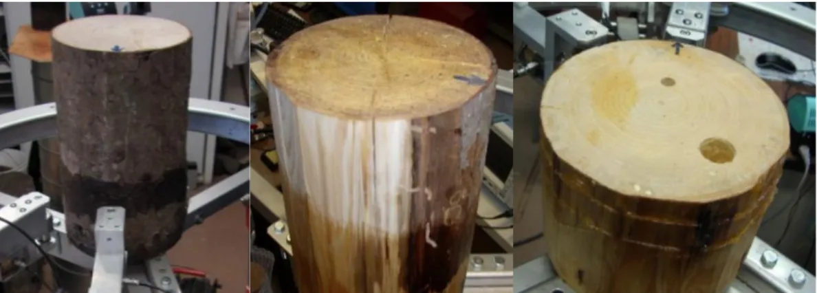
The disk of 15 cm thick was tested in tomography with 3 states of the sample: bark, debarked and drilled (2 holes of diameter 1 cm and 2 cm, see Figure 2). The tomography tests were made with two repetitions and an angular step of 30° to estimate the measurement uncertainties and with an angular step of 10° for tomographic imaging.

Figure 2. Tomography tests on the first log (from left to right: bark, debarked and drilled with two holes of diameter 1 cm and 2 cm).

The second log was cut in two disks of thickness 15 cm. These disks were sampled in the middle area of the log. In each disk a hole of diameter 5 cm was drilled, one in the middle and the second off-centered (Figure 3). These two disks were tested in tomography with an angular step of 10°.

Figure 3. Tomography tests on the two disks of the second log (hole diameter of 5 cm).

2.3. Ultrasonic tomography

The ultrasonic tomograph consisted in an aluminium ring supported by a tripod (Figure 4) [3]. To be able to test small disks, a specific support was added and mounted between the tripod (Figure 3). This device was designed to test standing trees. Thus, the height of the ring can be adjusted from 1 m to 1.6 m but the typical height is 1.3 m. If the apparatus is mounted on a trunk (Figure 4) the two parts of the ring are first assembled, and then the tripod is fixed. The apparatus is then placed against the trunk using two narrowing elements. Each probe is mounted on a trolley and these trolleys are slipped within the ring. Finally, the last part of the ring is fixed and the third narrowing element is applied.

Figure 4. Mounting steps of the ultrasonic tomograph.

The probes had a frequency of 55 kHz and were designed for acoustic emission purpose. These probes were mounted on a specific support with a wheel and grease was used as coupling medium. The emission consisted in 5 square periods of 480 V. The output analog signal was amplified of 80 dB. The acquisition was performed by a converter of 16 bits resolution and a sampling frequency of 5

MHz. The duration of acquisition was set to 410 µs. The output signal was previously filtered by a Morlet wavelet at 55 kHz with a bandwidth of 20 kHz for denoising (Figure 5).

(a) (b)

Figure 5. Ultrasonic signal filtered by a Morlet wavelet at 55 kHz with a bandwidth of 20 kHz (a) and associated Fourier transform (b).

The ultrasonic parameters used for the image reconstructions were the slowness (s/m) and the attenuation (dB/m at 55 kHz). The slowness Sl was computed using cross correlation between the input and the output signals (Equation 2). The ratio between received energy and emitted energy was used to determine the attenuation At (Equation 3).

2

=

Max

(

_∫

e

( ) (

t

s

t

−

τ

)

d

τ

)

d

Sl

1

( )

( )

⎟

⎟

⎠

⎞

⎜

⎜

⎝

⎛

=

∫

∫

dt

t

e

dt

t

s

d

At

log

10

1

With Sl: the slowness, At: the attenuation, d: the distance between the emitter and the receiver, e(t): the input signal and s(t) the output signal.

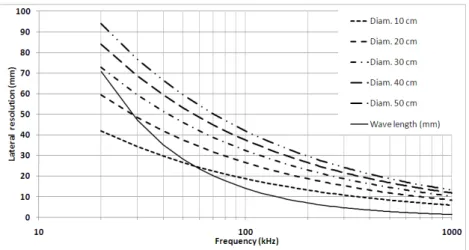
Figure 6. Lateral resolution and wavelength as a function of the frequency and according to the sample diameter (the acoustic wave speed was set to 1400 m/s).

The tomographic images were computed using an angular step of 10° which led to 900 acquisitions (36 equidistant acquisition points). A complete scan was done in 40 minutes with the apparatus. In comparison, three well trained operators were asked to make their own scan with 18 measurement points (306 acquisitions) and the duration of the scanning process was never less than one hour.

For a projection, the emitter is motionless while the receiver moves around the ring. The next projection is initiated by an angular step motion of the emitter followed by another motion of the receiver all around the ring (an acquisition is done at each angular step). The reconstruction algorithm was based on the inverse Radon transform in fan beam geometry (linear interpolation) with a modified Shepp-Logan filter. Considering the medium as isotropic, the elastic waves were assumed to propagate in a straight line. The velocity (and therefore the attenuation) of waves was then obtained from measurements of travel-time (of energy) differences by inverting the Radon transform.

The theoretical upper limit of the number of computed pixels was 450 (mesh of 39 mm², Equation 4). The physical resolution was however about 26 mm (axial resolution: wavelength) and 31 mm (lateral resolution: Fresnel zone, Equation 5, Figure 6). This resolution led to a mesh of 806 mm²; the images were thus 2D smoothed by a blackman filter of the wavelength size (the errors induced by the use of the modified Shepp-Logan filter was also highly reduced). It was important to highlight that the redundancy of the information (39 mm² compared to 806 mm²) allowed to decrease the effect of erroneous experimental values in the imaging process.

4

2

N

N

N

=

×

With NPixels: the number of pixels, NProjections: the number of projections (36), NSample: the number of

acquisitions per projection (25). 5

f

C

S

R

2

=

With RF: the Fresnel zone radius, Sd: the scanned depth (the rotation radius of the emitter or

receiver transducer), C: the wave celerity and f: the frequency of the transducer.

3. Results and discussion

In the next paragraphs, the slowness was presented in 103 _{(s/m) or its inverse: the speed in (m/s). The}

attenuation in (dB/m) was normalized by the diameter and thus presented in (dB).

3.1. Moisture content determination

The mean moisture content was 23% before the tests and 21% at the end of the experiment. The moisture content profile along the radius was presented at the Figure 7. The difference in moisture content from the pith to the bark was 5% before test and 10% after test. Despite the presence of the plastic film on the logs and on the disks, the wood samples tested were not in a green state and the natural drying effect increased while testing (phenomenon important after debarking). Small cracks appeared at the periphery of the disks due to drying (Figure 2, right image).

Figure 7. Moisture content (%) according to the radial position before and after the ultrasonic tests

(samples from the first log).

3.2. Measurement uncertainties

Two tomography tests were made with an angular step of 30° (108 acquisitions) on the same disk (with bark, debarked and drilled). The results were shown at the Figure 8 only for the disk with bark because the trends were very similar after debarking and drilling. Significant linear relationships were found for the speed (R² = 0.54, F = 105, p < 0.001, N = 108) and for the attenuation (R² = 0.93, F = 1373, p < 0.001, N = 108). The presence of outliers in the scatter plots of speed (Figure 8, a) was caused by errors in the travel time estimation. The standard error of the speed determination was thus ±420 m/s. The attenuation had a low measurement error compared to the speed estimation with a standard error equal to ±1.7 dB.

(a) (b)

Figure 8. Relationship between the two repetitions for (a) speed and (b) attenuation (disk with bark, N=108).

3.3. Effect of bark and holes on the ultrasonic parameters

Mean comparisons were made to study the effect of bark and holes on the ultrasonic parameters (Figure 9). The number of acquisitions was 108 with an angular step of 30°. The statistical tests were firstly a Student’s t-test on paired samples (Table 1).

(a) (b)

Figure 9. Means and standard deviations of speed (a) and attenuation (b) computed on 108 acquisitions for the disk with bark, debarked and drilled.

Table 1. t-Test and Wilcoxon test on paired samples for speed and attenuation between the disk with bark, debarked and drilled.

Data sets t ddl p-value (bilateral) Wilcoxon p (bilateral) Bark - Debarked Speed -1.934 107 0.056 0.496 Attenuation -5.888 107 < 0.001 < 0.001 Drilled – Debarked Speed 2.196 107 0.030 0.126 Attenuation -0.059 107 0.953 0.998

The t-test results, presented in Table 1, were biased by the non normal distribution of the parameters. To highlight this phenomenon, two histograms were plotted (Figure 10) after the tomographic tests with an angular step of 10° (N=900). The bimodal distribution was shown on this figure for speed with two modes between 1200 (m/s). The same type of distribution was also observed concerning the attenuation between -51 (dB). Equivalent observations were made for the debarked and drilled disks.

(a) (b)

Figure 10. Histograms of speed (a) and attenuation (b) of acoustic waves at 55 kHz computed for the disk with bark (N=900).

The results of Table 1 were secondly completed by non-parametric Wilcoxon tests (valid when the normality assumption was not satisfied or the sample size was too small). The Wilcoxon tests agreed with those of Student’t for attenuation but did not confirm the Student’t results for speed (Table 1). The mean attenuation measured on the disk with bark was thus significantly different with the one after debarking. The mean attenuation was higher with bark than without bark. No significant difference was found between the mean attenuation of debarked disk and of drilled disk. Concerning the speed measurements, differences existed between disks with bark, debarked and drilled but the probability values were too high to be absolutely affirmative (Figure 9 and Table 1).

3.4. Relationship between slowness and attenuation

The Figure 11 showed a scatter plot between slowness and attenuation for the disk with bark. A significant linear relationship was found with a R² equal to 0.51 (F=933, p < 0.001, N=900). The attenuation increased when the slowness increased or the speed decreased. However, the degree of fit should be read with care because the Figure 11 clearly showed two populations (associated with the distributions of the Figure 10). Outliers were also visible due to the uncertainty on the slowness determination; but they were not associated to particular positions of the probes.

3.5. Tomographic images

The computed maps of slowness and attenuation for the first log with and without the bark were presented at Figure 12. The images were displayed in 87x87 pixels and based on a 10° angular step (900 acquisitions). There was no visible effect of the presence of the bark on the outlines of the maps (Figure 12). This phenomenon was due to the low thickness of the bark (3 to 5 mm) compared to the wavelength (26 mm) added with the smoothing effect of the 2D filter.

(a) (c)

(b) (d)

Figure 12. Tomographic maps of slowness (10-3 _{s/m) (a, b) and attenuation (dB) (c, d) for the disk}

of the first log, with bark (a, c) and debarked (b, d).

The Figure 12 showed however two different areas from the pith to the periphery. These areas were highlighted at Figure 13 where the paths were drawn if the slowness was lower than 1.2x10-3 _{s/m and}

if the attenuation was upper than -51 dB. The periphery was thus characterized by a higher speed and a lower damping than the ones of the pith.The inverse phenomenon was observed by Socco and interpreted as an effect of the wood anisotropy [14]. The shorter paths (periphery) were more influenced by the tangential behavior of wood, while the radial behavior had a more important effect for longer paths (center). However, the radial velocity of wood is known to be upper than the tangential velocity. In this specific case (Figure 12), this observation was explained by the transition from juvenile to mature wood coupled with the effect of the moisture distribution (Figure 7).

(a) (b)

Figure 13. Paths of emitter to receiver with a slowness lower than 1.2x10-3 _{s/m (a) and an}

attenuation upper than -51 dB (b) for the disk of the first log with bark.

(a) (b)

Figure 14. Tomographic maps of slowness (10-3 _{s/m) (a) and attenuation (dB) (b) for the drilled disk}

of the first log. The black circles indicate the positions of the drillings.

The tomographic images obtained for the drilled disks of the two logs were presented at Figure 14 and Figure 15. The effect of the holes was visible on the maps by areas with a high slowness and also a high damping. This observation was valid even for the hole which diameter (10 mm) was the half of the wavelength (26 mm). It seemed that the position of holes in the disk had an effect on the reconstructed pattern; the holes closed to the pith were characterized by two elliptic patterns at the difference of those closed to the periphery. The shape of the patterns associated with the holes was not a circle but an ellipse and several hypotheses were advanced: the anisotropy was not taken into account, some cracks due to natural drying occurred, the reconstruction procedure was not well adapted for missing data (the dimension of the probe supports not allowed to scan the total angular area but only 250° for each projection), the mounting of the probes (Figure 5, right image) induced back waves which altered the received signals. These hypotheses will be investigated in a future study to improve the tomographic process.

(a) (d)

(b) (e)

(c) (f)

Figure 15. Tomographic maps of slowness (10-3 _{s/m) (b, e) and attenuation (dB) (c, f) for the two}

disks of the second log (a, b).

4. Conclusions

An automatic tomograph device specifically designed for standing trees was presented. The scanning process employed constituted an improvement compared to previous works. This improvement was a fast process with only two probes leading to scans with an angular precision of 10 degrees without the intervention of an operator during the process. This tomograph was used on two logs of spruce (Pica

abies) to study the effect of the bark and also the effect of defects like holes on the reconstructed

images. The tests were not done at a green state with mean moisture content of 22% and a gradient of 7% between the pith and the periphery. The ultrasonic parameters used for imaging of wood were

slowness and attenuation. The use of attenuation was not reported in previous works and a better accuracy of determination was found compared to slowness. It appeared that time of flight determination was less accurate even when cross correlation was employed. This phenomenon was due to the dispersion and the dissipation of wood material which caused a high attenuation coupled with modifications of the incident waves. The means of the ultrasonic parameters were not sufficient to discriminate the presence of defects in trees, but the presence of the bark had a significant contribution in the signal attenuations. For the tested samples, it was shown that speed near the bark was higher than in the pith because of the presence of juvenile wood coupled with the moisture gradient (natural drying occurred during the tests). In the same way, the damping near the bark was lower than in the center. A significant relationship between slowness and attenuation was shown but the population was bimodal due to the presence of juvenile wood. It was however possible to observe that a high speed was coherent with a low damping. The presence of the bark was not visible on the tomographic images. This was probably due to its small thickness compared to the wavelength. The presence of the holes was however clearly visible but artifacts did not permit a precise shape reconstruction and localization. Removing these artifacts will be the objective of future developments.

5. Acknowledgments

The BIOGMID project was supported by a grant from the French National Research Agency (BLAN07-1_183692, “BioGMID”).

References

1] Barnett J., Jeronimidis G. 2003. Wood Quality and its Biological Basis (Wiley-Blackwell). 2] Beall F.C., 2002. Overview of the use of ultrasonic technologies in research on wood properties.

Wood Sci. Technol. 36:197–212.

3] Brancheriau L., Gallet P., Thaunay P., Lasaygues P. (2009). Ultrasonic device for the imaging of green wood. 6th Plant Biomechanics Conference – Cayenne, France, November 16–21, 285-288.

4] Bucur V., 2003. Techniques for high resolution imaging of wood structure: a review. Meas. Sci. Technol. 14:R91-R98.

5] Deflorio G., Fink S., Schwarze F., 2008. Detection of incipient decay in tree stems with sonic tomography after wounding and fungal inoculation. Wood Sci. Technol. 42:117–132.

6] Dikrallah A., Kabouchi B., Hakam A., Brancheriau L., Baillères H., Famiri A., Ziani M. 2010. Study of acoustic wave propagation through the cross section of green wood. C. R. Mecanique 338(2): 107-112.

7] Divos F., Divos P. 2005. Resolution of stress wave based acoustic tomography. 14th International Symposium on Nondestructive Testing of Wood, Hannover, Germany: 309-314. 8] Lin C., Kao Y., Lin T., Tsai M., Wang S., Lin L., Wang Y., Chan M., 2008. Application of an

ultrasonic tomographic technique for detecting defects in standing trees. International Biodeterioration & Biodegradation 62(4):434-441.

9] Maurer H.R., Schubert S.I., Baechle F., Clauss S., Gsell D., Dual J., and Niemz P., 2006. A simple anisotropy correction procedure for acoustic wood tomography. Holzforschung 60:567– 573.

10] Nicolotti, G., L.V. Socco, R. Martinis, A. Godio, and L. Sambuelli. 2003. Application and comparison of three tomographic techniques for detection of decay in trees. Journal of Arboriculture 29:66–78.

11] Rinn F. 2004.Holzanatomische Grundlagen der Schall-Tomographie an Bäumen. Neue Landschaß 7:44-47.

12] Schmoldt D.L. 1996. CT imaging, data reduction, and visualization of hardwood logs. Proc. 24th Annual Hardwood Symposium, Meyer D A ed. National Lumber Assoc. Cashiers, North

Carolina: 69-80.

13] Schubert S. 2007. Acousto-ultrasound assessment of inner wood decay in standing trees: possibilities and limitations. Diss ETH Nr. 17126, Zürich.

14] Socco L.V., Sambuelli L., Martinis R., Comino E., Nicolotti G. 2004. Feasibility of ultrasonic tomography for nondestructive testing of decay on living trees. Research in Nondestructive Evaluation, 15(l):31-54.

15] Wang X., Allison R.B., Wang L., Ross R.J., 2007. Acoustic tomography for decay detection in red oak trees. Research Paper FPL-RP-642. Madison, WI: U.S. Department of Agriculture, Forest Service, Forest Products Laboratory. 7 p.

16] Wang X., Divos F., Pilon C., Brashaw B.K., Ross R.J., Pellerin R.F. 2004. Assessment of decay in standing timber using stress wave timing nondestructive evaluation tools: A guide for use and interpretation. Gen. Tech. Rep. FPL-GTR-147. Madison, WI: U.S. Department of Agriculture, Forest Service, Forest Products Laboratory. 12 p.

17] Wang X., Wiedenbeck J., Ross R.J., Forsman J.W., Erickson J.R., Pilon C., Brashaw B.K. 2005. Nondestructive evaluation of incipient decay in hardwood logs. Res. Pap. FPL–GTR–162. WI: U.S. Department of Agriculture, Forest Service, Forest Products Laboratory, 11 p.