Modelling a Cessna 337G hybrid-electric aircraft using Modelica: battery thermodynamics & cooling

(1)

Publisher’s version / Version de l'éditeur:

Vous avez des questions? Nous pouvons vous aider. Pour communiquer directement avec un auteur, consultez la première page de la revue dans laquelle son article a été publié afin de trouver ses coordonnées. Si vous n’arrivez pas à les repérer, communiquez avec nous à PublicationsArchive-ArchivesPublications@nrc-cnrc.gc.ca.

Questions? Contact the NRC Publications Archive team at

PublicationsArchive-ArchivesPublications@nrc-cnrc.gc.ca. If you wish to email the authors directly, please see the first page of the publication for their contact information.

https://publications-cnrc.canada.ca/fra/droits

L’accès à ce site Web et l’utilisation de son contenu sont assujettis aux conditions présentées dans le site LISEZ CES CONDITIONS ATTENTIVEMENT AVANT D’UTILISER CE SITE WEB.

Laboratory Technical Report (National Research Council of Canada. Flight

Research Laboratory); no. LTR-FRL-2021-0006, 2021-01-22

READ THESE TERMS AND CONDITIONS CAREFULLY BEFORE USING THIS WEBSITE. https://nrc-publications.canada.ca/eng/copyright

NRC Publications Archive Record / Notice des Archives des publications du CNRC :

https://nrc-publications.canada.ca/eng/view/object/?id=89246e39-8da8-4178-908f-4189b85e9889

https://publications-cnrc.canada.ca/fra/voir/objet/?id=89246e39-8da8-4178-908f-4189b85e9889

NRC Publications Archive

Archives des publications du CNRC

For the publisher’s version, please access the DOI link below./ Pour consulter la version de l’éditeur, utilisez le lien DOI ci-dessous.

https://doi.org/10.4224/40002055

Access and use of this website and the material on it are subject to the Terms and Conditions set forth at

Modelling a Cessna 337G hybrid-electric aircraft using Modelica:

battery thermodynamics & cooling

(2)

Modelling a Cessna 337G Hybrid-Electric

Aircraft using Modelica: Battery

Thermodynamics & Cooling

Crain, A., Gibney, E., and Zdunich, P.

Aviation Recorder Technologies Group

Flight Research Lab

January 22

th

, 2021

Volume: 1 Report Number: LTR-FRL-2021-0006

(3)

ISBN X-XXX-XXXXX-X

(4)

Abstract

Analytical simulation software tools are used to predict the behavior of an aircraft in various situations that may be difficult or undesirable to achieve in flight. This can provide important insight into aircraft behaviors, which can improve pilot proficiency and safety. This is especially true for unconventional or highly modified aircraft, which do not yet have proven performance. This report presents the research and development of a simulation capability at the National Research Council Canada for an unconventional aircraft, namely the twin-engine aircraft procured and modified to support the Hybrid Electric Aircraft Testbed (HEAT) project. Historically, the NRC has used imperative programming languages to perform aircraft simulations (MATLAB/Simulink, C++, and Fortran 77). Unlike past simulators developed at the NRC, the simulation capability described in this report was developed using Modelica-Dymola; Modelica is an open-source, declarative programming language in which the objective of the program is defined, but not the control flow. This allows the program to be acausal, which allows for multi-domain interactions between the aircraft dynamics, the electrical components of the powertrain, the thermodynamics of the batteries, and the fluid dynamics of the cooling system.

Towards this modelling objective, discharge curves were obtained experimentally for the 120 Ah battery modules used in the HEAT aircraft. The discharge curves informed the development of an open-circuit voltage exponential-polynomial model, which simulated battery voltage as a function of instantaneous current draw and battery state-of-charge when used in an equivalent circuit model. The geometric properties of the module were used to develop a physical model of the battery, allowing for simulations of the battery module (and cell) surface temperatures. These geometric measurements were combined with publically available measurements of certain thermodynamic parameters to further refine the model. The thermodynamics model was validated against preliminary experimental data collected during discharge. The model of the battery cooling arrangement to be used on the HEAT aircraft was developed in Modelica, and the complete battery model was integrated with the existing simulation capabilities. Simulations were performed for the expected flight profile, and the cell core temperatures were within the operational range of the cells used.

(5)

List of Symbols

English Letters

𝐴 Area 𝑚 Mass

𝐴𝑏 Battery model polynomial coefficients 𝑛𝑠 Number of cells in series

𝐴𝑠 Surface area 𝑁𝑢 Nusselt number

𝐶𝑝 Specific heat capacity 𝑃 Power

𝐶 Capacitance 𝑃𝑟 Prandtl Number

𝐷𝑐, 𝐿𝑐, 𝑊𝑐 Depth, length, and width of cell 𝑞 Heat flux

𝐷𝑝, 𝐿𝑝, 𝐻𝑝 Depth, length, and width of battery

module 𝑄 Capacity

𝑔 Gravity constant 𝑅 Resistance

𝐺𝑐 Convective thermal conductance 𝑅𝑒 Reynolds number

ℎ Convection coefficient 𝑅𝑎 Rayleigh number

𝑖 Current 𝑇 Temperature

𝑘 Conduction coefficient 𝑡 Time

𝑘𝑓 Thermal conductivity 𝑣 Voltage

𝑘𝑥, 𝑘𝑦, 𝑘𝑧 Convection coefficient in x, y, and z 𝑉 Volumetric Flow Rate or Volume

𝐾𝑒𝑥𝑝, 𝐾𝑧 Battery model exponential coefficients 𝑧 State-of-Charge

Greek Letters

𝛼 Thermal diffusivity

𝛽 Thermal expansion coefficient

𝜈 Kinematic viscosity

Accents

(6)

List of Acronyms and Initialisms

DLR German Aerospace Center

EME Energy, Mining and Environment

ECM Equivalent Circuit Model

GUI Graphical User Interface

HEAT Hybrid Electric Aircraft Test-bed

NACA National Advisory Committee for Aeronautics

ODE Ordinary Differential Equation

OCV Open-Circuit Voltage

RPM Rotations per Minute

SOC State-of-Charge

(7)

List of tables

Table 1: 120 Ah Cell Specifications ... 18

Table 2: 120 Ah Thermal Specifications ... 18

Table 3: 120 Ah Pack Specifications ... 18

Table 4: Thermal Properties of Aluminum (Cell Casing, Module Base, and Cakepan) ... 22

Table 5: Thermal Properties of Thermal Silicone... 22

Table 6: Thermal Properties of Electrical Insulation ... 22

Table 7: Thermal Properties of Thermal Pad ... 22

Table 8: Extended Flight Profile (1) ... 26

Table 9: Extended Flight Profile (2) ... 26

Table 10: 16 & 14-Module Reduced Flight (with Go-Around) ... 31

(9)

List of figures

Figure 1: Open-circuit Voltage, State-of-charge Dependence, Equivalent Series Resistance, and Diffusion

Voltage (Left to Right) ... 11

Figure 2: Modelica Implementation of ECM ... 13

Figure 3: Experimental Discharge Curves of the HEAT project’s 120 Ah cells ... 14

Figure 4: Simulated vs. Experimental Discharge Curves ... 16

Figure 5: 120 Ah Li-Ion Cell Representation ... 17

Figure 6: Drawing of the 120 Ah Battery Pack ... 18

Figure 7: Simplified Slice of 120 Ah Battery Pack and Enclosure ... 19

Figure 8: Wall Conduction Model ... 20

Figure 9: Modelica Implementation of Mass with Conduction ... 21

Figure 10: Cell Conduction Model ... 21

Figure 11: Pack Conduction Model ... 23

Figure 12: Pack Convection ... 24

Figure 13: Modelica Implementation of Convection Model ... 25

Figure 14: Forced Air Convection Experimental Setup ... 26

Figure 15: Discharge Profile Load Current ... 27

Figure 16: Discharge Profile Power ... 27

Figure 17: Modelica Representation of EME-Vancouver Experiment (Free Convection) ... 27

Figure 18: Simulation vs. Experiment - Free Convection ... 28

Figure 19: Simulation vs. Experiment - Forced Convection ... 28

Figure 20: CAD Model of Battery Stack ... 29

Figure 21: NACA 009-MU-A Inlet ... 29

Figure 22: NACA Inlets & Exits Slits ... 30

Figure 23: Simulated Current Draw – Reduced Flight ... 32

Figure 24: Simulated Core Temperature – Reduced Flight ... 32

Figure 25: Simulated Airspeed - Reduced Flight ... 32

Figure 26: Simulated Altitude - Reduced Flight ... 32

Figure 27: Simulated Current Draw – Extended Flight ... 33

Figure 28: Simulated Core Temperature – Extended Flight ... 33

(10)

Figure 30: Simulated Altitude - Extended Flight... 34 Figure 31: Extended Flight SOC ... 34

(11)

1 Introduction

Modern aircraft are becoming increasingly fuel efficient through progressively fine-tuned engine designs, in a bid to reduce costs and increase sustainability. However, it is becoming increasingly evident that the future of propulsion no longer lies in the further development of fossil fuel-based engines, but instead lies in the development of more sustainable fully-electric propulsion systems. This evolution cannot occur all at once, as the development of electric aircraft will require a complete rethinking of modern aircraft systems. This includes, but is not limited to, the requirement to increase specific and volumetric battery energy density dramatically to make them viable for use in a fully-electric aircraft. To lay the groundwork, a current trend in aviation is in the research and development of hybrid-electric aircraft, which lay somewhere between the designs of traditional aircraft and the modern aspiration of fully-electric aircraft.

To ensure that the NRC has the capabilities to support industry in this emerging field, the Hybrid-Electric Aircraft Testbed (HEAT) project was proposed in early 2017. To facilitate the growth of these capabilities, the aim of the project was to gain practical experience in the process of installing an electric motor onto an aircraft. More specifically, a Cessna 337G – a push-pull aircraft – was procured and the rear engine was to be replaced with a fully-electric powertrain, including the installation of an electric motor and a battery module. Through the development of the electric powertrain, real-world experience in the installation of electric motors and power supplies in an aircraft were gained, including developing adequate cooling and safety strategies which could help inform industry and regulators.

In the context of HEAT, the development of an analytical software simulation tool was desired to perform safety critical analyses prior to the first flight of the modified aircraft. The simulator tool was to incorporate all necessary aspects of the hybrid-electric aircraft, including the aerodynamics of the aircraft, the discharge performance and thermodynamics of the battery modules, the performance of the cooling solution, and the thrust generated by the electric powertrain. This document covers the development of the battery model and all associated components, using the Modelica language [1]. It is divided according to the different aspects of the model developed: the electrical model, the thermodynamics model, the battery cooling model, and the simulations performed using the integrated simulation tool, which includes the aerodynamics model developed in Reference [2].

(12)

2 Battery Modelling (Electrical)

In this section, the modelling of the 120 Ah battery discharge performance is described. The model is an equivalent-circuit model (ECM), which is not meant to describe the construction of the cell. Rather, it acts as a description of the cell’s high-level behavior. The various components described in this section (resistors, capacitors, etc.…) are not actually present inside a cell, but instead act as analogues to some of the internal processes. Additional information can be found in Reference [3]. The various improvements described in the following subsections are also shown in Figure 1.

Figure 1: Open-circuit Voltage, State-of-charge Dependence, Equivalent Series Resistance, and Diffusion Voltage (Left to Right)

2.1 Open-Circuit Voltage Theory

In order to develop an ECM, it is necessary to first describe open-circuit voltage (OCV) theory. As described in Reference [3], the model was first built to represent the cell as an ideal source of voltage. Consider the following: if a voltmeter is placed on the terminals of a cell, a voltage will be registered. This represents the open-circuit voltage for the current state-of-charge (SOC) of the cell, as it does not take into account the effect of load current or of past usage. This type of model is not accurate enough for most purposes, as in reality cell voltage is dependent on the load current, recent usage, and many other factors. The OCV model selected for the HEAT simulator is the sum of an exponential term and a generic polynomial:

OCV(𝑧(𝑡)) =𝐾𝑒𝑥𝑝exp(𝐾𝑧𝑧(𝑡)) + ∑4𝑖=1𝐴_𝑏𝑖𝑧𝑖−1(𝑡) (1)

The parameters of this model (highlighted in red) were identified using experimental discharge curves for the 120 Ah batteries. However, the discharge data collected is not the OCV, as there is a load current required to discharge the battery. So, a model which considers the dynamics of the battery was developed using the techniques described in the following subsections. The OCV parameters were then identified using parameter estimation tools in Dymola by comparing the model output to the experimental data.

(13)

2.2 State-of-Charge Dependence

State-of-charge dependence is the most logical improvement to the OCV model. This is done by defining “charge status”; in other words, the SOC of a cell is 100% (1.0) when fully charged and 0% (or 0.0) when fully discharged. The SOC is a unitless quantify represented by 𝑧. To obtain the SOC, the total capacity of a cell is required – in this case 120Ah - and it is symbolized by 𝑄. Total capacity is a constant for a cell, though does decrease due to aging and can be accelerated by various non-optimal operating conditions. The change in SOC can be obtained using the following ordinary differential equation (ODE):

𝑧̇(𝑡) = −𝜂(𝑡)𝑖(𝑡)𝑄−1 ₍₂₎

In this ODE, 𝜂(𝑡) is the charge efficiency which has a value of unity when discharging. During charging, 𝜂(𝑡) ≤ 1 because a small fraction of the charge passing through the cell participates in unwanted side-reactions which do not increase the cell’s SOC. An accurate model of the charge efficiency is non-trivial, and for the purposes of the HEAT simulator was set to unity during charging. Normally, the discrete-time equivalent of this equation would be required to perform simulations. However, the simulation capability described in this report was developed in Modelica, which only requires the ODE in continuous time. During compilation, Modelica can solve the ODE’s in real-time [1].

2.3 Equivalent Circuit Resistance

The model thus far is technically “static”, as it only describes the behavior of the cell at rest. The next step is to add in the dynamics of the cell, which define the behavior of the cell when subjected to a time-varying load. When a load is applied to a cell, the observed behavior is that the terminal voltage drops below the OCV during discharge and rises above the OCV during charge. This can be modelled using a resistor in series with the controlled voltage source. In this modified circuit, the equation for SOC remains the same, however a second equation defining the terminal voltage as a function of current input and resistance is required:

𝑣(𝑡) = OCV(𝑧(𝑡))−𝑖(𝑡)𝑅0 (3)

The function defining the terminal voltage as a function of SOC is typically determined in a laboratory environment through repeated experiments. This resistance implies that power is dissipated by the cell’s internal resistance, and thus the efficiency of the cell is imperfect. This dissipated power is referred to as Joule heating, and is defined by:

𝑃(𝑡) = 𝑖2_(𝑡)𝑅

0 (4)

This model is suitable for simple circuit design problems, but is not adequate for large scale applications such as the electric powertrain in the HEAT aircraft.

2.4 Diffusion Voltages

The term “polarization” refers to any variation in the cell’s terminal voltage away from the OCV as a result of current passing through the cell. Thus far, the polarization of the cell has been modeled as instantaneous

(14)

through the 𝑖(𝑡)𝑅0 term. In reality, the behavior of a cell is more complex, with the voltage polarization

changing more slowly over time as current is demanded from the cell, and then decaying slowly over time immediately following the end of the load current. This phenomenon is caused by the slow diffusion processes of lithium in a lithium-ion cell. The simplest way to model this effect is by using at least one parallel resistor-capacitor sub-circuit. Again, the SOC equation remains the same, but the voltage equation becomes:

𝑣(𝑡) = OCV(𝑧(𝑡)) − 𝑅1𝑖𝑅1(𝑡) − 𝑅0𝑖(𝑡) (5)

Where:

𝑖𝑅1(𝑡) = 𝑖(𝑡) − 𝐶1𝑣̇𝐶1 (6)

Once again, Modelica makes the solution to these ODEs trivial, requiring only that a suitable number of ODEs be defined by the user. There are a few other improvements that can be made to the model (Warburg impedance, hysteresis voltages, SOC-varying hysteresis, etc.…), but it was decided that the model at this stage would be suitable for the first order simulations required by the HEAT project. Future work may entail improving the model with the additions listed previously.

2.5 Modelica Implementation

Implementing the model in Modelica was done in two steps. First, the OCV model described in Section 2.1 was written in the Modelica language – see Appendix A: OCV Model. The second step was to integrate the OCV model into a model that contained both the equivalent resistance and diffusion voltage effects. In Dymola this involved building the electrical circuit shown in Figure 1 using the components from the Modelon electrical library [4], as shown in Figure 2.

(15)

This model, when properly tuned using experimental data, can be used to estimate the dynamics of the cell as a function of SOC and current draw. Details on the thermal aspect of the model are described in Section 3, but it should be noted that the coreTemperature and heatFlow blocks are sensor blocks which output the temperature and heat flow produced through the resistor via Joule’s Law; this is referred to as the “core temperature” in this report, as it is the temperature at the most central volumetric point of the model.

2.6 Parameter Estimation

To use the model described in Section 2.5, parameter estimation was performed. These parameters were 𝑅1, 𝐶1, 𝑅0, 𝐾𝑒𝑥𝑝, 𝐾𝑧, and 𝐴𝑏_𝑖; parameter estimation was performed in Dymola using the Optimization

library. In brief, the Optimization library “provides tools to benefit from numerical optimization algorithms without special knowledge about the internals of the algorithms. It helps to conveniently setup optimization runs by tailored Graphical User Interfaces (GUIs) for different tasks. For example, you are able to automatically optimize model parameters in order to improve the system performance assessed by some model variables” [5]. The Optimization library was developed by the German Aerospace Center (DLR), and the library version used in this analysis was version 2.2.4 (2019-03-13, build 4). In addition Modelica version 3.2.3 was used, in conjunction with Dymola 2021.

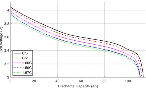
The experimental discharge data was collected by NRC’s Energy, Mining, and Environment (EME) group in Vancouver, BC. The battery was discharged at 30 A, 60 A, 120 A, 180 A, and 200 A in a 20°C temperature controlled chamber, with no direct cooling on the surface of the battery. Between each discharge cycle the battery was charged at 40 A to a maximum cell voltage of 4.1 V. The resulting discharge curves at the various load currents are shown in Figure 3. This figure also demonstrates the behavior of the cell as described in Section 2.3; that is to say, the voltage measured at a given SOC changes as a function of the current draw.

(16)

Using this experimental data and the ECM, the high-level automated procedure to obtain the parameters was:

 Simulate the model for the various load cases (C/3, C/2, 1C, 1.5C, 1.67C) using an initial guess of the model parameters.

 Calculate the error between the model and the data using the 𝑙2_{-norm (cost function).}

𝑙𝑛𝑜𝑟𝑚2 = √∑𝑛𝑘=1|Error𝑘|2 (7)

 Calculate the gradient of the cost function.

 Calculate the change in parameter value using the Optimization library algorithm.

Through this procedure, the following parameter values were estimated for the OCV model described in Eq. (1):

 𝐾𝑒𝑥𝑝 = −512.9

 𝐾𝑧= −69.7

 𝐴𝑏= [3.15, 1.88, −2.85, 1.91]

The parameters for the overall ECM were estimated to be:  𝑅1= 0.006 Ω

 𝐶1= 1 F

 𝑅0= 0.0026 Ω

Comparing the model performance to the experimental data in Figure 4, the simulations match the experimental discharge curves sufficiently well for the purposes of the HEAT simulator, with the exception of the discharge performance below approximately 30% SOC; below this SOC, the simulation diverges from the experimental results. However, given that the HEAT simulator is not expected to be used for that range of operation, it was deemed acceptable.

(17)

(18)

3 Battery Modelling Theory (Thermodynamics)

In this section, the thermodynamic modelling used for each cell is described. The primary means of heat generation in the cells was assumed to be Joule heating (Eq. (4)). Joule’s Law calculates the power generated due to resistance, which is proportional to the heat flow from the resistor if one assumes that all electrical losses in the resistor are converted into heat. Perfect heat conduction between each layer of a cell was assumed (i.e. no air gap unless specifically mentioned).

3.1 Thermal Model

A brief review of heat conduction is described in this subsection. The equation for conduction rate is given by Reference [6]:

𝑞𝑥 = 𝑘𝐴Δ𝑡Δ𝑥−1 (8)

Thus, the heat rate in the 𝑥-direction is a function of the temperature gradient between both sides of the cell, the area of the surface perpendicular to the 𝑥-direction, and the thermal conductivity of the material. For the HEAT simulator, the conductivity of each material is assumed to be a constant. The 120 Ah cell is represented in Figure 5.

Figure 5: 120 Ah Li-Ion Cell Representation

The geometric and thermal parameters for the 120 Ah cells in the HEAT battery module are summarized in Table 1 and Table 2, and were either measured directly or taken from literature [7, 8, 9, 10]. In the following tables, [M] identifies a measured parameter and [L] identified a parameter pulled from literature.

(19)

Table 1: 120 Ah Cell Specifications Parameter Value Nominal Voltage 3.68 V [M] Nominal Capacity 120 Ah [M] Max Voltage 4.15 V [M] Length (𝐿𝑐) 173 mm [M] Width (𝑊𝑐) 125 mm [M] Depth (𝐷𝑐) 45 mm [M] Weight 2.01 kg [M]

Table 2: 120 Ah Thermal Specifications

Parameter Value Specific Heat Capacity (𝐶𝑃) 1091 J/(kg K) [L] Thermal Conductivity (𝑘𝑥) 31.4 W/(m k) [L] Thermal Conductivity (𝑘𝑦) 126.35 W/(m K) [L] Thermal Conductivity (𝑘𝑧) 0.735 W/(m K) [L]

Having described the individual cell at a high level, it’s necessary to describe the pack. The battery module consists of twelve 120 Ah cells connected in series, as shown in Figure 6:

Figure 6: Drawing of the 120 Ah Battery module

The specifications at the pack level are summarized in Table 3:

Table 3: 120 Ah Pack Specifications

Parameter Value Nominal Voltage 44.04 V [M] Nominal Capacity 120 Ah [M] Max Voltage 50.38 V [M] Length (𝐿𝑐) 305 mm [M] Width (𝑊𝑐) 384 mm [M] Depth (𝐷𝑐) 133 mm [M] Weight 29.52 kg [M]

(20)

To properly visualize the structure of the cell, which facilitates the Modelica implementation, consider a slice of the battery module as shown in Figure 7:

Figure 7: Simplified Slice of 120 Ah Battery Module and Enclosure

When developing the model, certain assumptions were made:

 The primary cooling surface is the aluminum cakepan at the bottom of the battery module. Minimal convective cooling was assumed to occur on any of the other surfaces.

 Thermal interactions were assumed to be 1-D, i.e. a series of lump masses, and the thermodynamics were not discretized in any way. This significantly simplified the computational efficiency of the model at the cost of model accuracy. As a result of this, the “core” is treated as an infinitesimal point at the center of the cell, as opposed to the complex anode-cathode-electrolyte configuration which will not generate heat at a single point.

 The aluminum cell casing is electrically continuous and therefore generates some heat via 𝐼2_𝑅

losses. This is also the case with the bus bars interconnecting the cells. Neither one of these sources of heat generation are captured, which may result in lower than expected temperatures

(21)

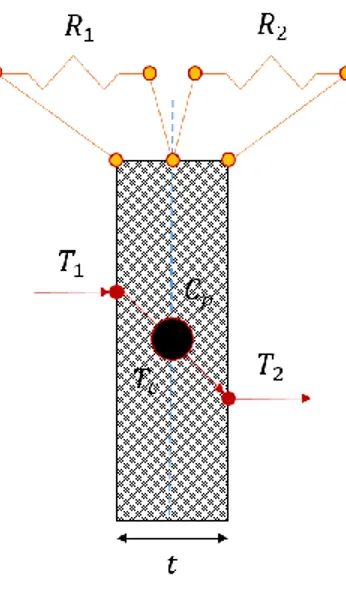
Each of the conduction interfaces described in Figure 7 has been defined as a wall of some thickness, thermal capacity, and thermal resistance, as shown in Figure 8.

Figure 8: Wall Conduction Model

The classical conduction equation (Eq. (8)) can be modified such that it retains heat due to its thermal capacity. The resistance of each wall segment can be obtained through:

𝑅 = 𝑡(𝐴 𝑘)−1 ₍₉₎

Heat flow through the resistive surface is then obtained through:

𝑄̇1→𝑐 = (𝑇𝑐− 𝑇1)𝑅1−1 (10)

The above equation can then be simplified to the classical conduction equation. The heat flow through the thermal mass is calculated using:

𝑄̇ = (𝑇𝑐− 𝑇1)𝐶𝑝𝑚 (11)

Where the mass of the wall is obtained from the known material properties and the dimensions of the wall. The heat flow at the other side of the wall is calculated from:

𝑄̇𝑐→2 = (𝑇2− 𝑇𝑐)𝑅2−1 (12)

3.2 Modelica Implementation

These equations are straightforward to implement in Modelica. First, a conductive body in Modelica (using pre-built Modelica functions) takes the form shown in Figure 9:

(22)

Figure 9: Modelica Implementation of Mass with Conduction

This model serves as the foundation for the full thermodynamics of the cell. The full cell model can be assembled using the mass with conduction model as shown in Figure 10.

Figure 10: Cell Conduction Model

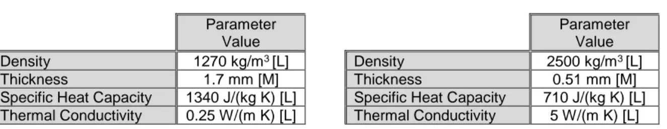
The heat generated via Joule’s Law enters this model through the corePort input, which is connected to the input ports of the surrounding conductive masses (each of which are identical to Figure 9, with different physical properties). Heat propagates through the layers as described by Figure 7, and the thermal and geometric properties of each mass is described in Table 4 through Table 7. In reality, the closest measurement of the core temperature are the terminals, which are modelled through the

(23)

Table 4: Thermal Properties of Aluminum (Cell Casing, Module Base, and Cakepan)

Parameter Value Density 2710 kg/m3 _[L]

Thickness 1 mm [L] Specific Heat Capacity 1256 J/(kg K) Thermal Conductivity 167 W/(m K)

Table 5: Thermal Properties of Thermal Silicone

Thickness 0.66 mm [M] Specific Heat Capacity 711 J/(kg K) [L] Thermal Conductivity 0.08 W/(m K) [L]

Table 6: Thermal Properties of Electrical Insulation

Thickness 1.7 mm [M] Specific Heat Capacity 1340 J/(kg K) [L] Thermal Conductivity 0.25 W/(m K) [L]

Table 7: Thermal Properties of Thermal Pad

Thickness 0.51 mm [M] Specific Heat Capacity 710 J/(kg K) [L] Thermal Conductivity 5 W/(m K) [L]

The full pack model was then constructed from the cell model in Figure 10 by defining the material interfaces between each cell, as well as the conductive connection between the positive and negative terminals. The assembled Modelica model is shown in Figure 11. In the pack model, each cell is connected to any adjacent cells to model their thermally conductive interactions. For example, cell #11 (top left) is connected to cell #12 (top right) via the right-left cell interface, and to cell #10 via the front-back interface. In addition, each cell is also connected via their terminals. Lastly, the heat flow input from the bottoms of all cells are collected together using the Modelica thermalCollector function, which sums the heat flow and assumes it flows through a single point (which is then subsequently connected to the aluminum cakepan).

(24)

Figure 11: Pack Conduction Model

Long Side

thermalCollectorFront m=2 thermalCollectorBack m=2 bottomPlateHeat corePort[] frontLongSidePort backLongSidePort leftShortSidePort rightShortSidePort

(25)

4 Battery Cooling

In this section, details regarding the cooling of the battery module will be provided. This includes both the theory on convection and an overview of the Modelica implementation.

4.1 Convection Model

To cool the battery, air flow over the bottom surface is utilized. While the batteries are not expected to exceed the pre-defined temperature thresholds during the flight, it was still necessary to develop a cooling model to further confirm what was observed in experiment. The classical convection equation is given by [11]:

𝑞 = ℎ̅𝐴𝑠(𝑇𝑠− 𝑇∞) (13)

Thus, the heat flow due to convection is a function of the exposed area, the average convection coefficient, and the difference between the surface temperature and the temperature of the fluid at infinity. In a convection problem, the most difficult parameter to estimate is the convection coefficient. For the purpose of the HEAT simulator it was assumed that the cakepan (the primary cooling surface as shown in Figure 7) was a flat plate, and that air flow is parallel to the plate, as shown:

Figure 12: Pack Convection

It was also assumed that the air flow over the battery module is turbulent, given that the air flow is the result of 4 NACA ducts pulling in air from the outside of the aircraft, where the air is allowed to flow freely in the cabin until it is pulled out from slits in the rear cabin windows. To estimate the average convective coefficient for turbulent flow over a flat plate, the following equation was used [12]:

𝑁𝑢𝐿

̅̅̅̅̅̅ = (0.037𝑅𝑒_𝐿

4

5_{− 841) 𝑃𝑟}1₃ ₍₁₄₎

(26)

𝑅𝑒𝐿 = 𝑉𝐿

𝜈 (15)

And the Prandtl number was obtained from: 𝑃𝑟 =𝜈

𝛼 (16)

Once the Nusselt number was obtained, the average convection coefficient was calculated: ℎ̅ =𝑘𝑓𝑁𝑢̅̅̅̅̅̅𝐿

𝐿 (17)

In order to estimate the convection coefficient for free convection, the following empirical model was used:

𝑁𝑢𝐿 ̅̅̅̅̅̅ = 0.68 + 0.67𝑅𝑎_𝐿14_{(1 + (}0.492 𝑃𝑟 ) 9 16 ) −4₉ (18)

Where 𝑅𝑎𝐿 is known as the Rayleigh number, which can be calculated from:

𝑅𝑎𝐿 =

𝑔𝛽(𝑇𝑠−𝑇∞)𝐿3

𝜈𝛼 (19)

The parameters used in these equations are typically a function of temperature and pressure. The HEAT simulator utilized Dymola’s built in models for dry air, and the values of the parameters will not be summarized in this report. For a complete overview of the parameter values for air, Reference [12] provides complete tables covering air from 100 K to 3000 K.

4.2 Modelica Implementation

The convection model was primarily implemented into Modelica programmatically, as opposed to being constructed from pre-existing components. At a high level the Modelica model takes the form:

Figure 13: Modelica Implementation of Convection Model

In this model, the speed of the air flow over the aluminum plate was used as an input to the convection model, while the output was the convective thermal conductance 𝐺𝑐, which is simply the area of the plate

multiplied by the average convection coefficient. The Modelica code for this model is located in Appendix B: Convection Model.

(27)

4.3 Experimental Validation

The model was validated against experimental data generated by EME-Vancouver. However, this validation data was generated early in the project and was performed without the battery enclosure and thermal pad. This is evident in Figure 14, which shows the battery without the titanium shroud and aluminum cakepan in place. The model was therefore modified by removing the material for the enclosure from all sides to capture this difference.

A representative discharge was performed on a single battery module in a temperature controlled environment with a small fan pushing air (at 2.28 m/s) parallel to the bottom of the battery module, shown in Figure 14.

Figure 14: Forced Air Convection Experimental Setup

The discharge profile is an extended profile that consists of a 39 minute flight with a climb, cruise, descent, and go-around. Details on the profile are shown in Table 8 and

Table 9.

Table 8: Extended Flight Profile (1)

Segment Power (kW) Propeller (RPM) TAS (knots)

Takeoff / Initial Climb 155.3 (100%) 2800 96

Climb 155.3 (100%) 2800 96 Cruise 108.1 (65%) 2600 145 Descent 69.1 (41%) 2400 - Go-Around Climb 155.3 (100%) 2800 - Go-Around Cruise 108.1 (65%) 2600 145 Go-Around Descent 69.1 (41%) 2400 -

Table 9: Extended Flight Profile (2)

Segment Altitude (ft) Duration (s) Total Time (min)

Takeoff / Initial Climb - 26 0.4

Climb - 41 1.1

Cruise 1000 453 8.7

Descent - 100 10

(28)

Go-Around Cruise 1000 85 12.3

Go-Around Descent - 70 13.2

The current draw for the profile is shown in Figure 15 and the power is shown in Figure 16:

Figure 15: Discharge Profile Load Current Figure 16: Discharge Profile Power

Using the components developed in the previous sections, the following Modelica model was developed:

(29)

Comparing the temperatures measured on the bottom of the battery and cell terminal to the simulated results (for the free convection case), the results compare sufficiently well for the purposes of the HEAT simulator.

Figure 18: Simulation vs. Experiment - Free Convection Figure 19: Simulation vs. Experiment - Forced Convection

Despite the positive agreement between the results, some interesting observations can be made:

 The bottom of the simulated battery module appears to heat up slightly more than in experiment for the free convection scenario. This is likely due to the simplicity of the thermal model, and additional accuracy may be obtained by discretizing the model.

 It is apparent that despite the application of cool air on the bottom of the battery, the temperature of the terminal only decreases by approximately 1-2 °C compared to the case without such air flow. This indicates that air-cooling the battery – unless there is a significant difference between the air temperature and the battery temperature – is not likely to have a significant impact on the internal temperature.

 Considering the lack of 𝐼2_{𝑅 losses in the cell interconnects, the terminal temperatures match well.}

This indicates that the ambient air model may cool too aggressively compared to experiment. Future testing and measurements will aid in refining both models.

4.4 Aircraft Cooling System

Following the successful validation of the thermodynamic model for a single battery module, the next step expanded the model to the full 16 module battery stack (Figure 20).

(30)

Figure 20: CAD Model of Battery Stack

When developing this model in Modelica, it was assumed that no heat transfer occurred between the 16 battery enclosures. Thus, the only additional component to model was the cooling system on the Cessna 337G. Cooling of the batteries on the Cessna is performed using 4 NACA 009-MU-A inlets on the side of the aircraft (Figure 21 and Figure 22).

(31)

Figure 22: NACA Inlets & Exits Slits

The flow rate from these NACA ducts can be calculated using the speed of the aircraft and the area of the ducts. The inlets are 3.5” by 1”, and the volumetric flow rate equation is:

𝑉𝑖𝑛 = 𝑣𝑖𝑛𝐴𝑖𝑛𝑙𝑒𝑡 (20)

The air flow over each battery was conservatively assumed to be 1/8 of the total volumetric flow rate, given the 8 batteries per row in the rack. This is conservative as it assumes the two modules on the port and starboard receive the air from only two NACA ducts. The area between each battery row is 0.0258 m2_{, the}

Modelica implementation of this function is trivial and will not be shown, but consider the following sample calculation at cruise: 𝑣𝑏𝑎𝑡𝑡 = 4𝑣𝑐𝑟𝑢𝑖𝑠𝑒𝐴𝑖𝑛𝑙𝑒𝑡 8𝐴_{𝑏𝑎𝑡𝑡} = 4 ∗ 74.55 ∗ (0.0889 ∗ 0.0254) ∗ (8 ∗ 0.0258) −1_{= 3.26 m/s} (21)

(32)

5 Simulations

In this section, the results from three simulated flight profiles are shown; a 16-pack reduced flight (with a go-around), a 14-module reduced flight (with go-around), and a 16-module extended flight (with go-around). The simulations were performed using the aerodynamic model developed in Reference [2] as well as the models described in this report.

5.1 Reduced Scope Flight

The 14 and 16-module profiles are described in Table 10. The Modelica implementation of these simulations will not be presented in this report due to their complexity. For all simulations, it was assumed that the ambient air temperature remained constant at 20°C.

Table 10: 16 & 14-Module Reduced Flight (with Go-Around)

Segment Power (kW) Propeller (RPM) TAS (knots) Altitude (ft) Duration (s) Total Time (min) Takeoff / Initial Climb 155.3 (100%) 2800 96 - 26 0.4 Climb 155.3 (100%) 2800 96 - 41 1.1 Cruise 108.1 (65%) 2600 145 1000 453 8.7 Descent 69.1 (41%) 2400 - - 100 10 Go-Around Climb 155.3 (100%) 2800 - - 35 10.6 Go-Around Cruise 108.1 (65%) 2600 145 1000 85 12.3 Go-Around Descent 69.1 (41%) 2400 - - 70 13.2

(33)

Figure 23: Simulated Current Draw – Reduced Flight Figure 24: Simulated Core Temperature – Reduced Flight

Figure 25: Simulated Airspeed - Reduced Flight Figure 26: Simulated Altitude - Reduced Flight

These results demonstrate that for the reduced scope flight, the core temperature of the batteries should not be of concern, as the peak temperature during the go-around was 30.3°C for the 14-module case and this is well below the maximum desired temperature. Note that the operational temperature range for the batteries is 40-60°C. However, the current draw for the 14-module case may decrease the lifespan of the batteries, and should a 14-module be configuration be considered for the flight, it is recommended that additional testing be performed on the batteries to ensure the increase in current draw does not risk damaging the cells, both in the short term and in the long term.

5.2 Extended Flight

(34)

Table 11: 16-Module Reduced Flight (with Go-Around) Segment Power (kW) Propeller (RPM) IAS/TAS (knots) Altitude (ft) Duration (s) Total Time (min) Takeoff / Initial Climb 155.3 (100%) 2800 96 - 83 1.4 Reduced Power Climb 123.3 (85%) 2600 74 - 254 5.6 Cruise 108.1 (65%) 2600 150 5000 1113 24.2 Descent 69.1 (41%) 2400 - - 500 32.5 Go-Around Climb 155.3 (100%) 2800 - - 47 33.2 Go-Around Cruise 108.1 (65%) 2600 145 1000 203 36.7 Go-Around Descent 69.1 (41%) 2400 - - 125 38.8

The simulation results for the extended flight profile are shown in Figure 27 - Figure 30:

(35)

Figure 29: Simulated Airspeed - Extended Flight Figure 30: Simulated Altitude - Extended Flight

These results demonstrate that the battery temperature is not expected to exceed 37.4°C during the extended flight, which is still below the maximum acceptable temperature for the batteries. Note this peak temperature is less than that shown experimentally in Section 4.3 despite the inclusion of the battery module enclosures in the model. This is due to the inclusion of a low-power descent segment in these simulations, during which time the battery temperature does not increase. In this case, it is also interesting that the go-around is initiated at approximately 35% SOC (Figure 31), which provides the pilots with sufficient charge to complete the go-around and land.

Figure 31: Extended Flight SOC

(36)

6 Conclusions & Next Steps

In this report, the HEAT simulator was expanded to include the battery model, both in terms of discharge performance and thermal output. Details of the discharge model were provided, including the parameters estimated for the equivalent circuit model, which were obtained using nonlinear parameter estimation and experimental data. The thermodynamic theory for the lithium ion cells was outlined and a Modelica model was developed to leverage the acausal nature of the software. The individual cell models were used to build module models, and then further expanded to the full 16-module pack. The thermodynamics model was validated against experimental data collected by EME-Vancouver, and the results compared favourably. The Modelica implementation of the aircraft cooling system for the batteries was also presented, and preliminary data suggests that the simple convection model is a sufficiently accurate model for the purposes of the HEAT simulator. The discharge, thermodynamics, and cooling Modelica models were integrated with the aerodynamics model previously developed for the HEAT simulator. Using the integrated simulator, flight profiles were defined and simulated to obtain estimates of the expected battery temperatures and power requirements. These results were used to inform future testing of the batteries at EME-Vancouver and to provide confidence that the batteries will operate within the desired temperature range in flight. To further improve the HEAT simulator, the electric powertrain must be developed and validated against experimental data.

(37)

7 References

[1] The Modelica Association, "Modelica," 20 January 2020. [Online]. Available: https://www.modelica.org/. [Accessed 20 April 2020].

[2] A. Crain and E. G. Patrick Zdunich, "Modelling a Cessna 337G Hybrid-Electric Aircraft using Modelica: Aerodynamics," National Research Council Canada, Ottawa, 2021.

[3] G. Plett, Battery Modelling, Norwood: Artech House, 2015.

[4] Modelon, "Electrification Library," [Online]. Available: https://www.modelon.com/library/electrification-library. [Accessed 28 01 2021].

[5] German Aerospace Center, "Systems & Control Innovation Lab," [Online]. Available: https://www.systemcontrolinnovationlab.de/the-dlr-optimization-library/.

[6] Y. Cengel and A. Ghajar, Heat and Mass Transfer - Fundamentals & Applications, 4th ed., New York: McGraw-Hill, 2007.

[7] K. Chen, Heat Generation Measurments of Prismatic Lithium Ion Batteries, Waterloo: University of Waterloo, 2013.

[8] ASTM International, " Standard Test Method for Thermal Conductivity of Solids by Means of the Guarded-Comparative-Longitudinal Heat Flow Technique," 2009.

[9] S. Neupane, Experimental and Modeling Study of Electrochemical and Thermal Behavior of Lithium-ion Batteries, Kansas: University of Kansas, 2014.

[10] A. Lidbeck and K. Syed, Experimental Characterization of Li-ion Battery Cells for Thermal Management in Heavy Duty Hybrid Applications, Gothenburg: Chalmers University of Technology, 2017.

[11] B. Munson, T. Okiishi, W. Huebsch and A. Rothmayer, Fundamentals of Fluid Mechanics, 7th ed., New Jersey: John Wiley & Sons, Inc., 2013.

(38)

Appendix A: OCV Model

model Lithium_Ion_OVC_120Ah

"A model of a simple lithium − ion cell using an equivalent circuit model. "

// Model parameters for the open − voltage exponential − polynomial model

parameter Real exp_gain = − 512.9032258064515872 "Exponential term gain"annotation (Dialog(group = "OVC Properties"));

parameter Real exp_SoC = − 69.6627565982404633 "State − of − charge exponent"annotation (Dialog(group = "OVC Properties"));

parameter Real A[: , : ] = [3.1544477028347995, 1.8758553274682308,

−2.849462365591398, 1.9149560117302054] "Polynomial coefficient matrix"annotation (Dialog(group = "OVC Properties"));

// Define the cell specific parameters

parameter Real Q_cell = 120 ∗ 3600 "Cell capacity"annotation (Dialog(group = "OVC Properties"));

parameter Real SOC_init = 1.0 "Initial cell state − of − charge"annotation (Dialog(group = "OVC Properties")); // Define the number of cells in series:

parameter Integer ns = 1 "Number of cells in series"annotation (Dialog(group = "Battery module Properties")); parameter Integer np = 1 "Number of cells in parallel"annotation (Dialog(group = "Battery module Properties"));

Real i(quantity = "Current", unit = "A") "Current"; Real v(quantity = "Voltage", unit = "V") "Total voltage"; Real vCell(quantity = "Voltage", unit = "V") "Cell voltage";

final parameter Modelica. SIunits. ElectricCharge Q_bat = Q_cell ∗ np "Battery charge";

Modelica. SIunits. ElectricCharge Q_curr(start = SOC_init ∗ Q_bat, fixed = true) "Current charge"; Modelica. Electrical. Analog. Interfaces. PositivePin pin_p "Positive pin"

annotation (Placement(transformation(extent = {{−10,98}, {10,118}})));

Modelica. Electrical. Analog. Interfaces. NegativePin pin_n "Negative pin"

annotation (Placement(transformation(extent = {{−10, − 118}, {10, −98}})));

Modelica. Blocks. Interfaces. RealOutput SOC "State − of − charge"annotation (Placement( transformation(

extent = {{−10, −10}, {10,10}}, rotation = 180,

origin = {−114,0})));

equation

assert( Q_cell > 0, "Cell capacity is negative. ", AssertionLevel. error); assert( SOC > 0, "Cell state − of − charge is negative. ", AssertionLevel. error); assert( v > 0, "Battery voltage is negative. ", AssertionLevel. error);

assert( vCell > 0, "Cell voltage is negative. ", AssertionLevel. error); // Calculate voltage: v = pin_p. v − pin_n. v; 0 = pin_p. i + pin_n. i; i = pin_p. i; // Charge model: der(Q_curr) = i;

(39)

SOC = min(Q_curr, Q_bat)/Q_bat;

// Volage lookup as a function of state − of − charge:

vCell = exp_gain ∗ exp(exp_SoC ∗ SOC) + sum({A[1, i] ∗ SOC^(i − 1) for i in 1:size(A, 2)}); v = vCell ∗ ns;

(40)

Appendix B: Convection Model

𝑚𝑜𝑑𝑒𝑙 𝐴𝑖𝑟𝐶𝑜𝑜𝑙𝑖𝑛𝑔𝑀𝑜𝑑𝑒𝑙_𝑇𝑢𝑟𝑏𝑢𝑙𝑒𝑛𝑡𝑃𝑎𝑟𝑎𝑙𝑙𝑒𝑙𝐹𝑙𝑜𝑤 "𝐸𝑚𝑝𝑖𝑟𝑖𝑐𝑎𝑙 𝑚𝑜𝑑𝑒𝑙 𝑜𝑓 𝑎𝑖𝑟 𝑐𝑜𝑜𝑙𝑖𝑛𝑔 𝑝𝑟𝑜𝑝𝑒𝑟𝑡𝑖𝑒𝑠 𝑎𝑠 𝑎 𝑓𝑢𝑛𝑐𝑡𝑖𝑜𝑛 𝑜𝑓 𝑣𝑒𝑙𝑜𝑐𝑖𝑡𝑦. " 𝑝𝑎𝑟𝑎𝑚𝑒𝑡𝑒𝑟 𝑅𝑒𝑎𝑙 𝐿 = 0.3874 "𝑃𝑙𝑎𝑡𝑒 ℎ𝑒𝑖𝑔ℎ𝑡"; 𝑝𝑎𝑟𝑎𝑚𝑒𝑡𝑒𝑟 𝑅𝑒𝑎𝑙 𝑊 = 0.3048 "𝑃𝑙𝑎𝑡𝑒 𝑤𝑖𝑑𝑡ℎ"; 𝑝𝑎𝑟𝑎𝑚𝑒𝑡𝑒𝑟 𝑅𝑒𝑎𝑙 𝐾𝑣 = 15.89𝑒 − 6 "𝐾𝑖𝑛𝑒𝑚𝑎𝑡𝑖𝑐 𝑣𝑖𝑠𝑐𝑜𝑠𝑖𝑡𝑦 𝑜𝑓 𝑎𝑖𝑟 @ 300 𝐾, 𝑃 = 1.013"; 𝑝𝑎𝑟𝑎𝑚𝑒𝑡𝑒𝑟 𝑅𝑒𝑎𝑙 𝑇𝑑 = 22.5𝑒 − 6 "𝑇ℎ𝑒𝑟𝑚𝑎𝑙 𝑑𝑖𝑓𝑓𝑢𝑠𝑖𝑣𝑖𝑡𝑦 𝑜𝑓 𝑎𝑖𝑟 @ 300 𝐾, 𝑃 = 1.013"; 𝑝𝑎𝑟𝑎𝑚𝑒𝑡𝑒𝑟 𝑅𝑒𝑎𝑙 𝑘 = 26.3𝑒 − 3 "𝑇ℎ𝑒𝑟𝑚𝑎𝑙 𝑐𝑜𝑛𝑑𝑢𝑐𝑡𝑖𝑣𝑖𝑡𝑦 𝑜𝑓 𝑎𝑖𝑟 @ 300 𝐾, 𝑃 = 1.013"; 𝑝𝑎𝑟𝑎𝑚𝑒𝑡𝑒𝑟 𝑅𝑒𝑎𝑙 𝑔 = 9.81 "𝐺𝑟𝑎𝑣𝑖𝑡𝑦 𝑐𝑜𝑛𝑠𝑡𝑎𝑛𝑡"; 𝑅𝑒𝑎𝑙 ℎ; 𝑅𝑒𝑎𝑙 𝐴; 𝑅𝑒𝑎𝑙 𝑃𝑟; 𝑅𝑒𝑎𝑙 𝑅𝑒_𝐿; 𝑅𝑒𝑎𝑙 𝑁𝑢_𝐿; 𝑅𝑒𝑎𝑙 𝑅𝑎_𝐿; 𝑅𝑒𝑎𝑙 𝑇𝑓; 𝑅𝑒𝑎𝑙 𝐵; 𝑀𝑜𝑑𝑒𝑙𝑖𝑐𝑎. 𝐵𝑙𝑜𝑐𝑘𝑠. 𝐼𝑛𝑡𝑒𝑟𝑓𝑎𝑐𝑒𝑠. 𝑅𝑒𝑎𝑙𝐼𝑛𝑝𝑢𝑡 𝑣; 𝑀𝑜𝑑𝑒𝑙𝑖𝑐𝑎. 𝐵𝑙𝑜𝑐𝑘𝑠. 𝐼𝑛𝑡𝑒𝑟𝑓𝑎𝑐𝑒𝑠. 𝑅𝑒𝑎𝑙𝑂𝑢𝑡𝑝𝑢𝑡 𝐺𝑐; 𝑀𝑜𝑑𝑒𝑙𝑖𝑐𝑎. 𝐵𝑙𝑜𝑐𝑘𝑠. 𝐼𝑛𝑡𝑒𝑟𝑓𝑎𝑐𝑒𝑠. 𝑅𝑒𝑎𝑙𝐼𝑛𝑝𝑢𝑡 𝑇𝑖𝑛𝑓; 𝑀𝑜𝑑𝑒𝑙𝑖𝑐𝑎. 𝐵𝑙𝑜𝑐𝑘𝑠. 𝐼𝑛𝑡𝑒𝑟𝑓𝑎𝑐𝑒𝑠. 𝑅𝑒𝑎𝑙𝐼𝑛𝑝𝑢𝑡 𝑇𝑠; 𝑒𝑞𝑢𝑎𝑡𝑖𝑜𝑛 𝑃𝑟 = 𝐾𝑣/𝑇𝑑; 𝑅𝑒_𝐿 = (𝑣 ∗ 𝐿)/𝐾𝑣; 𝑇𝑓 = (𝑇𝑠 + 𝑇𝑖𝑛𝑓)/2; 𝐵 = 1/𝑇𝑓; 𝑅𝑎_𝐿 = (𝑔 ∗ 𝐵 ∗ (𝑇𝑠 − 𝑇𝑖𝑛𝑓) ∗ 𝐿^3)/(𝐾𝑣 ∗ 𝑇𝑑); 𝑖𝑓 𝑅𝑒_𝐿 < 1𝑒2 𝑡ℎ𝑒𝑛 𝑁𝑢_𝐿 = 0.68 + (0.670 ∗ 𝑅𝑎_𝐿^(1/4))/((1 + (0.492/𝑃𝑟)^(9/16))^(4/9)); 𝑒𝑙𝑠𝑒𝑖𝑓 𝑅𝑒_𝐿 <= 5𝑒5 𝑎𝑛𝑑 𝑅𝑒_𝐿 >= 1𝑒2 𝑡ℎ𝑒𝑛 𝑁𝑢_𝐿 = 0.664 ∗ (𝑅𝑒_𝐿^(1/2)) ∗ (𝑃𝑟^(1/3)); 𝑒𝑙𝑠𝑒𝑖𝑓 𝑅𝑒_𝐿 > 5𝑒5 𝑡ℎ𝑒𝑛 𝑁𝑢_𝐿 = (0.037 ∗ 𝑅𝑒_𝐿^(4/5) − 841) ∗ 𝑃𝑟^(1/3); 𝑒𝑙𝑠𝑒 𝑁𝑢_𝐿 = 0; 𝑒𝑛𝑑 𝑖𝑓; ℎ = 𝑁𝑢_𝐿 ∗ (𝑘/𝐿); 𝐴 = 𝐿 ∗ 𝑊; 𝐺𝑐 = 𝐴 ∗ ℎ; 𝑒𝑛𝑑 𝐴𝑖𝑟𝐶𝑜𝑜𝑙𝑖𝑛𝑔𝑀𝑜𝑑𝑒𝑙_𝑇𝑢𝑟𝑏𝑢𝑙𝑒𝑛𝑡𝑃𝑎𝑟𝑎𝑙𝑙𝑒𝑙𝐹𝑙𝑜𝑤;

(41)

𝑚𝑜𝑑𝑒𝑙 𝐴𝑖𝑟𝐶𝑜𝑜𝑙𝑖𝑛𝑔𝑀𝑜𝑑𝑒𝑙_𝑃𝑒𝑟𝑝𝑒𝑛𝑑𝑖𝑐𝑢𝑙𝑎𝑟𝐹𝑙𝑜𝑤 "𝐸𝑚𝑝𝑖𝑟𝑖𝑐𝑎𝑙 𝑚𝑜𝑑𝑒𝑙 𝑜𝑓 𝑎𝑖𝑟 𝑐𝑜𝑜𝑙𝑖𝑛𝑔 𝑝𝑟𝑜𝑝𝑒𝑟𝑡𝑖𝑒𝑠 𝑎𝑠 𝑎 𝑓𝑢𝑛𝑐𝑡𝑖𝑜𝑛 𝑜𝑓 𝑣𝑒𝑙𝑜𝑐𝑖𝑡𝑦. " 𝑝𝑎𝑟𝑎𝑚𝑒𝑡𝑒𝑟 𝑅𝑒𝑎𝑙 𝐷 = 0.3874 "𝑉𝑒𝑟𝑡𝑖𝑐𝑎𝑙 𝑝𝑙𝑎𝑡𝑒 ℎ𝑒𝑖𝑔ℎ𝑡"; 𝑝𝑎𝑟𝑎𝑚𝑒𝑡𝑒𝑟 𝑅𝑒𝑎𝑙 𝑊 = 0.3048 "𝑉𝑒𝑟𝑡𝑖𝑐𝑎𝑙 𝑝𝑙𝑎𝑡𝑒 𝑤𝑖𝑑𝑡ℎ"; 𝑝𝑎𝑟𝑎𝑚𝑒𝑡𝑒𝑟 𝑅𝑒𝑎𝑙 𝐶 = 0.228 "𝐻𝑖𝑙𝑝𝑒𝑟𝑡 𝑐𝑜𝑛𝑠𝑡𝑎𝑛𝑡 𝑓𝑜𝑟 𝑛𝑜𝑛 − 𝑐𝑖𝑟𝑐𝑢𝑙𝑎𝑟 𝑠ℎ𝑎𝑝𝑒 𝑖𝑛 𝑐𝑟𝑜𝑠𝑠 − 𝑓𝑙𝑜𝑤 𝑜𝑓 𝑔𝑎𝑠"; 𝑝𝑎𝑟𝑎𝑚𝑒𝑡𝑒𝑟 𝑅𝑒𝑎𝑙 𝑚 = 0.731 "𝐻𝑖𝑙𝑝𝑒𝑟𝑡 𝑐𝑜𝑛𝑠𝑡𝑎𝑛𝑡 𝑓𝑜𝑟 𝑛𝑜𝑛 − 𝑐𝑖𝑟𝑐𝑢𝑙𝑎𝑟 𝑠ℎ𝑎𝑝𝑒 𝑖𝑛 𝑐𝑟𝑜𝑠𝑠 − 𝑓𝑙𝑜𝑤 𝑜𝑓 𝑔𝑎𝑠"; 𝑝𝑎𝑟𝑎𝑚𝑒𝑡𝑒𝑟 𝑅𝑒𝑎𝑙 𝐾𝑣 = 1.57𝑒 − 5 "𝐾𝑖𝑛𝑒𝑚𝑎𝑡𝑖𝑐 𝑣𝑖𝑠𝑐𝑜𝑠𝑖𝑡𝑦 𝑜𝑓 𝑎𝑖𝑟"; 𝑝𝑎𝑟𝑎𝑚𝑒𝑡𝑒𝑟 𝑅𝑒𝑎𝑙 𝑇𝑑 = 2.21𝑒 − 5 "𝑇ℎ𝑒𝑟𝑚𝑎𝑙 𝑑𝑖𝑓𝑓𝑢𝑠𝑖𝑣𝑖𝑡𝑦 𝑜𝑓 𝑎𝑖𝑟"; 𝑝𝑎𝑟𝑎𝑚𝑒𝑡𝑒𝑟 𝑅𝑒𝑎𝑙 𝑘 = 2.54𝑒 − 2 "𝑇ℎ𝑒𝑟𝑚𝑎𝑙 𝑐𝑜𝑛𝑑𝑢𝑐𝑡𝑖𝑣𝑖𝑡𝑦 𝑜𝑓 𝑎𝑖𝑟"; 𝑅𝑒𝑎𝑙 ℎ; 𝑅𝑒𝑎𝑙 𝐴; 𝑅𝑒𝑎𝑙 𝑃𝑟; 𝑅𝑒𝑎𝑙 𝑅𝑒_𝐷; 𝑅𝑒𝑎𝑙 𝑁𝑢_𝐷; 𝑀𝑜𝑑𝑒𝑙𝑖𝑐𝑎. 𝐵𝑙𝑜𝑐𝑘𝑠. 𝐼𝑛𝑡𝑒𝑟𝑓𝑎𝑐𝑒𝑠. 𝑅𝑒𝑎𝑙𝐼𝑛𝑝𝑢𝑡 𝑣; 𝑀𝑜𝑑𝑒𝑙𝑖𝑐𝑎. 𝐵𝑙𝑜𝑐𝑘𝑠. 𝐼𝑛𝑡𝑒𝑟𝑓𝑎𝑐𝑒𝑠. 𝑅𝑒𝑎𝑙𝑂𝑢𝑡𝑝𝑢𝑡 𝐺𝑐; 𝑒𝑞𝑢𝑎𝑡𝑖𝑜𝑛 𝑃𝑟 = 𝐾𝑣/𝑇𝑑; 𝑅𝑒_𝐷 = (𝑣 ∗ 𝐷)/𝐾𝑣; 𝑁𝑢_𝐷 = 𝐶 ∗ (𝑅𝑒_𝐷^𝑚) ∗ (𝑃𝑟^(1/3)); 𝑖𝑓 𝑣 > 0 𝑡ℎ𝑒𝑛 ℎ = 𝑁𝑢_𝐷 ∗ (𝑘/𝐷); 𝑒𝑙𝑠𝑒 ℎ = 12; 𝑒𝑛𝑑 𝑖𝑓; 𝐴 = 𝐷 ∗ 𝑊; 𝐺𝑐 = 𝐴 ∗ ℎ; 𝑒𝑛𝑑 𝐴𝑖𝑟𝐶𝑜𝑜𝑙𝑖𝑛𝑔𝑀𝑜𝑑𝑒𝑙_𝑃𝑒𝑟𝑝𝑒𝑛𝑑𝑖𝑐𝑢𝑙𝑎𝑟𝐹𝑙𝑜𝑤;

(42)