HAL Id: hal-01084505
https://hal.inria.fr/hal-01084505
Submitted on 19 Nov 2014
HAL is a multi-disciplinary open access
archive for the deposit and dissemination of
sci-entific research documents, whether they are
pub-lished or not. The documents may come from
teaching and research institutions in France or
abroad, or from public or private research centers.
L’archive ouverte pluridisciplinaire HAL, est
destinée au dépôt et à la diffusion de documents
scientifiques de niveau recherche, publiés ou non,
émanant des établissements d’enseignement et de
recherche français ou étrangers, des laboratoires
publics ou privés.
Partitioned conditional generalized linear models for
categorical data
Jean Peyhardi, Catherine Trottier, Yann Guédon
To cite this version:
Jean Peyhardi, Catherine Trottier, Yann Guédon. Partitioned conditional generalized linear models
for categorical data. 29th International Workshop on Statistical Modelling (IWSM 2014), Statistical
Modelling Society, Jul 2014, Göttingen, Germany. 4 p. �hal-01084505�
Partitioned conditional generalized linear
models for categorical data
Jean Peyhardi
1,2, Catherine Trottier
1, Yann Gu´
edon
21 Universit´e Montpellier 2, I3M, Montpellier, France 2
CIRAD, UMR AGAP and Inria, Virtual Plants, Montpellier, France E-mail for correspondence: [email protected]
Abstract: In categorical data analysis, several regression models have been pro-posed for hierarchically-structured response variables, such as the nested logit model. But they have been formally defined for only two or three levels in the hierarchy. Here, we introduce the class of partitioned conditional generalized lin-ear models (PCGLMs) defined for an arbitrary number of levels. The hierarchical structure of these models is fully specified by a partition tree of categories. Using the genericity of the (r, F, Z) specification of GLMs for categorical data, PCGLMs can handle nominal, ordinal but also partially-ordered response variables. Keywords: hierarchically-structured categorical variable; partition tree; partially-ordered variable; GLM specification.
1
(r,F,Z) specification of GLM for categorical data
The triplet (r, F, Z) will play a key role in the following since each GLM for categorical data can be specified using this triplet; see Peyhardi et al. (2013) for more details. The definition of a GLM includes the specification of a link function g which is a diffeomorphism from M = {π ∈ ]0, 1[J −1|PJ −1
j=1πj <
1} to an open subset S of RJ −1. This function links the expectation π =
E[Y |X=x] and the linear predictor η = (η1, ..., ηJ −1)t. It also includes
the parametrization of the linear predictor η, which can be written as the product of the design matrix Z (as a function of x) and the vector of parameters β. All the classical link functions g = (g1, . . . , gJ −1), rely on
the same structure which we propose to write as
gj = F−1◦ rj, j = 1, . . . , J − 1. (1)
where F is a continuous and strictly increasing cumulative distribution function (cdf) and r = (r1, . . . , rJ −1)t is a diffeomorphism from M to an
This paper was published as a part of the proceedings of the 29th Interna-tional Workshop on Statistical Modelling, Georg-August-Universit¨at G¨ottingen, 14–18 July 2014. The copyright remains with the author(s). Permission to repro-duce or extract any parts of this abstract should be requested from the author(s).
270 Partitioned conditional GLMs
open subset P of ]0, 1[J −1. Finally, given x, we propose to summarize a
GLM for a categorical response variable by the J − 1 equations r(π) = F (Zβ),
where F (η) = (F (η1), . . . , F (ηJ −1))T. In the following we will consider
four particular ratios. The adjacent, sequential and cumulative ratios re-spectively defined by πj/(πj+ πj+1), πj/(πj+ . . . + πJ) and π1+ . . . + πj
for j = 1, . . . , J − 1, assume order among categories but with different in-terpretations. We introduce the reference ratio, defined by πj/(πj+ πJ) for
j = 1, . . . , J − 1, useful for nominal response variables.
Finally, a single estimation procedure based on Fisher’s scoring algorithm can be applied to all the GLMs specified by an (r, F, Z) triplet. The score function can be decomposed into two parts, where only the first one depends on the (r, F, Z) triplet. ∂l ∂β = Z T ∂F ∂η ∂π ∂r | {z } (r,F,Z) dependent part Cov(Y |X = x)−1[y − π] | {z } (r,F,Z) independent part . (2)
We need only to evaluate the density function {f (ηj)}j=1,...,J −1to compute
the corresponding diagonal Jacobian matrix ∂F /∂η. For details on compu-tation of the Jacobian matrix ∂π/∂r according to each ratio, see Peyhardi (2013).
2
Partitioned conditional GLMs
The main idea consists in recursively partitioning the J categories then specifying a conditional GLM at each step. This type of model is therefore referred to as partitioned conditional GLM. Such models have already been proposed, such as the nested logit model (McFadden, 1978), the two-step model (Tutz, 1989) and the partitioned conditional model for partially-ordered set (POS-PCM) (Zhang and Ip, 2012). Our proposal can be seen as a generalization of these three models that benefits from the genericity of the (r, F, Z) specification. In particular, our objective is not only to pro-pose GLMs for partially-ordered response variables but also to differentiate the role of explanatory variables for each partitioning step using specific explanatory variables and design matrices. We are also seeking to formally define partitioned conditional GLMs for an arbitrary number of levels in the hierarchy.
PCGLM definition: Let J ≥ 2 and 1 ≤ k ≤ J − 1. A k-partitioned conditional GLM for categories 1, . . . , J is defined by:
• A partition tree T of {1, . . . , J } with V∗, the set of non-terminal
vertices of cardinal k. Let Ωv
j be the children of vertex v ∈ V∗.
• A collection of models C = {(rv, Fv, Zv(xv)) | v ∈ V∗} for
each conditional probability vector πv= (π1v, . . . , πvJv−1), where πv j =
P (Y ∈ Ωv
j|Y ∈ v; xv) and xv is a sub-vector of x associated with
vertex v.
PCGLM estimation: Using the partitioned conditional structure of model, the log-likelihood can be decomposed as l =P
v∈V∗lv, where lv represents
the log-likelihood of GLM (rv, Fv, Zv(xv)). Each component lvcan be max-imised individually, using (2), if all parameters {βv}
v∈V∗ are different.
PCGLM selection: The partition tree T and the collection of models C have to be selected using ordering assumption among categories.
• Nominal data: the partition tree T is built by aggregating similar categories - such as the nested logit model of McFadden (1978) - and C contains only reference models, appropriate for nominal data; see Peyhardi (2013).
• Ordinal data: we propose to adapt the Anderson’s indistinguishability procedure (1984) for PCGLM selection.
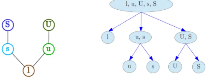
• Partially ordered data: the partial ordering assumption among cate-gories can be summarized by an Hasse diagram. Zhang and Ip (2012) defined an algorithm to build the partition tree T automatically from the Hasse diagram; see figure 1 with the pear tree dataset. It should be remarked that every partially-ordered variable Y can be expressed in terms of elementary ordinal and nominal variables ˜Yi(with at least
one ordinal variable). We propose to build the partition tree T di-rectly from these latent variables ˜Yi to obtain a more interpretable
structure. For these two methods of partition tree building, the main idea is to recursively partition the J categories in order to use a simple (ordinal or nominal) GLM at each step.
3
Application to pear tree dataset
Dataset description: In winter 2001, the first annual shoot of 50 one-year-old trees was described by node. The presence of an immediate axillary shoot was noted at each successive node. Immediate shoots were classified into four categories according to their length and transformation or not of the apex into spine (i.e. definite growth or not). The final dataset was thus constituted of 50 bivariate sequences of cumulative length 3285 combining a categorical variable Y (type of axillary production selected from among latent bud (l), unspiny short shoot (u), unspiny long shoot (U), spiny short shoot (s) and spiny long shoot (S)) with an interval-scaled variable X1
(internode length).
Results: A higher likelihood and simpler interpretations were obtained using partial ordering information. The axillary production Y of pear tree can be decomposed into two levels. Production first follows a sequential mechanism (ordinal model), giving latent bud, short shoot or long shoot
272 Partitioned conditional GLMs
(first level of hierarchy; figure 1), which is strongly influenced by the in-ternode length X1(the longer the internode, the longer the axillary shoot).
The axillary shoot apex then differentiates or not into spine (second level of hierarchy; figure 1) depending on distance to growth unit end (second explanatory variable X2expressed in number of nodes).
FIGURE 1. Hasse diagram and corresponding partition tree.
References
Anderson, J.A. (1984). Regression and ordered categorical variables. Jour-nal of the Royal Statistical Society, Series B, 46, 1 – 30.
McFadden, D. et al. (1978). Modelling the choice of residential location. Institute of Transportation Studies, University of California.
Peyhardi, J. (2013). A new GLM framework for analysing categorical data; application to plant structure and development. PhD thesis.
Peyhardi, J., Trottier, C. and Gu´edon, Y. (2013). A unifying framework for specifying generalized linear models for categorical data. In 28th In-ternational Workshop on Statistical Modeling, 331 – 335
Tutz, G. (1989). Compound regression models for ordered categorical data. Biometrical Journal, 31, 259 – 272.
Zhang, Q. and Ip, E.H. (2012). Generalized linear model for partially or-dered data. Statistics in Medicine.