Analysis & characterization of a flow thermo-electrochemical cell for power generation & heat convection

Analysis & Characterization of a Flow Thermo-electrochemical

Cell for Power Generation & Heat Convection

by

Ali Sina Booeshaghi

Submitted to the Department of Mechanical Engineering in partial fulfillment of the requirements for the degree of

Bachelor of Science in Mechanical Engineering MASSACHUSETTS INSTITUTE OF TECHNOLOGY at the

JUL 2

5

2017

MASSACHUSETTS INSTITUTE OF TECHNOLOGY

June 2017

LIBRARIES

Ali Sina Booeshaghi, MMXVII. All rights reserved.

ARCHIVES

The author hereby grants to MIT permission to reproduce and distribute publicly paper

and elec(tronic copies of this thesis document in whole or in part.

Signature redacted

A uthor.... ...

Department of Mechanical Engineering May 12, 2017

Certified

by

...

Signature redacted

...

Evelyn N. Wang Gail E. Kendall Associate Professor of Mechanical Engineering Thesis Supervisor

Signature redacted

Rohit Karnik

Associate Professor of Mechanical Engineering, Undergraduate Officer

The

author

hereby grants to MIT permission to

reproduce and to distribute publicly paper and

electronic copies of

this

thesis document in

whole or in part in any medium now known or

3

Analysis & Characterization of a Flow Thermo-electrochemical Cell for Power Generation & Heat Convection

by

Ali Sina Booeshaghi

Submitted to the Department of Mechanical Engineering on May 12, 2017, in partial fulfillment of the

requirements for the degree of

Bachelor of Science in Mechanical Engineering

Abstract

In this thesis, I analyzed and characterized a new flow thermo-electrochemical cell that generates power from waste-heat, while in parallel convecting this heat away from the source. I also re-viewed previous research on the topic of thermo-electric energy generation, governing physics behind thermo-electrochemical energy generation, actual device fabrication, device testing,

re-sults, and applications of this technology.

Thermo-electric devices (TE devices) exhibit the thermo-electric effect, where temperature gra-dients and material properties work in tandem to drive electron transfer at electrode surfaces, thereby generating electricity. For example, a typical sold-state TE device such as a bismuth tel-luride TE device, can generate up to 0.300 mV/K [31]. New reseach has emerged [25, 26, 14] focusing on liquid-based thermo-electrochemical (TEC) cells that take advantage of the temper-ature dependence of oxidation/reduction chemical reactions to generate electricity. One of the major benefits of these TEC devices over traditional TE devices is a much higher S, = 1.5 mV/K; another is the low cost of manufacturing, making them promising for commercial applications.

The new TEC device that I fabricated and studied utilizes a flowing electrolyte instead of a stationary electrolyte. With this new configuration, and a heated boundary condition, I studied both the energy generation and convective heat transfer capabilities of the flowing electrolyte TEC cell. Numerically I obtained a maximum power output and heat transfer coefficient for the TEC cell of Pmax = 2.6 pW and h = 340 W/m2K which corroborates well with the experimentally found value of Pmax = 2.0 pW and h = 450 W/m2. K.

If employed in data centers, as a device for CPU cooling, with the given power output I found that a 100,000 ft2 data center can generate about 21.96 MWh of energy, which at a cost of 0.20 $/kWh can save a data center about 5,000 $/year. More generally, the application of this technology in locations where waste-heat is prevalent, will allow for energy recycling and consequent cost savings.

Thesis Supervisor: Evelyn N. Wang

5

Acknowledgments

The author would like to acknoledge Professor Evelyn Wang for her guidance, Professor Baratunde Cola for his support and ideas, Ali H. Kazim for the collaboration, Heena Mutha for her sugges-tions, Solomon Adera for his mentorship, and his parents for unconditional love and support.

Contents

Contents 7

List of Figures 9

List of Tables 13

1 Introduction 15

1.1 Application for Energy Generation Devices . . . . 16

1.2 Thermo-electrochemical Cells . . . . 17

2 Governing Physics 21 2.1 Thermo-electric Effect . . . . 21

2.2 Thermo-electric Cells (TE Cells) . . . . 23

2.3 Thermo-electrochemical Cells (TEC Cells) . . . . 24

2.3.1 Electrodynamics . . . . 25

2.3.2 Heat Transfer & Fluid Mechanics . . . . 28

3 Device Fabrication & Experimental Setup 31 3.1 Design & Fabrication of the Cell . . . . 31

3.1.1 Iteration One . . . . 32

3.1.2 Iteration Two . . . . 33

3.2 Electrolyte Preparation . . . . 34

3.3 Experimental Setup . . . . 34

4 Device Performance 4.1 Numerical Analysis 4.1.1 Domain Setup 4.1.2 Results . . . . 4.2 Experimental Results 4.3 Discussion . . . .

5 Device Applications & Future Research Directions

5.1 D ata C enters . . . . 5.1.1 Cost A nalysis . . . . 5.2 Device Improvements . . . . Bibliography 39 39 39 41 44 47 49 49 50 50 53 . . . . . . . . . . . . . . . . . . . .

List of Figures

1-1 An example of a sTEC where charge migration is limited to diffusion and natural convection. The Fe(CN)63- ion gets reduces at the cold electrode and becomes

Fe(CN)64- then this ion gets oxidized at the hot electrode and returns to Fe(CN)6

3-

1-2 An example of a fTEC where charge migration is assisted by forced convection. The Fe(CN)63- ion gets reduces at the cold electrode, gets convected to the and

in the process heated by the boundary condition and then becomes Fe(CN)64 . . 18

2-1 Borup et al. shows different configurations for measuring the Seebeck coefficient of TE materials. (a) 2-point, (b) off-axis 4-point, and (c) on-axis 4-point. . . . . 23 2-2 The transition-metal complex of an Fe3+ ion bounded to six CN- ligands that

re-duce (gain an electron) to create another transition-metal complex of Fe2+ bounded to six CN- ligands, all in an octahedral geometry. . . . . 25 2-3 A crystal field theory energy diagram for the five d-orbitals of the Fe3+ ion. The

incoming electron will be placed in the dYZ orbital since electrons want to occupy the lowest energy state available. . . . . 26

3-1 The two iterations of the fTEC cell. From the first iteration of the cell (a) I made design modifications, such as a snaking fluid path, side inlet/outlet holes, and inline electrode holes so that iteration two (b) would provide a more accurate (and cleaner a.k.a. leakproof) function of the cell. . . . . 33 3-2 The multi-cord nylon seal with NPT thread was threaded into the top plate to

3-3 The two iterations of the fTEC cell after they have been machined. The main differ-ence between iteration one (a) and iteration two (b) are a longer flow path, smaller channels, and variable 2D electrode placement . . . . 35 3-4 A schematic of the experimental setup. Electrolyte gets pumped to the fTEC cell

by a peristaltic pump, the heater heats the electrolyte which consequently reacts at the electrode surfaces, generating a voltage. The system is closed loop, with the fluid resevoir maintained at a constant temperature. . . . . 36

3-5 The two iterations of the experimental setup for the fTEC Cell. The main difference between iteration one (a) and iteration two (b) are that the second iteration paid more careful attention to monitoring all variables in the system, one example is having a constant temperature bath for the inlet electrolyte. . . . . 37

4-1 The "differential" domain for my numerical analysis. The electrolyte flows in from the left, into the element, is exposed to a constant temperature boundary condition, oxidizes and reduces at the electrodes, and then exits the element. . . . . 40 4-2 (a) The steady state fully developed two dimensional temperature profile within

the electrolyte under a constant temperature boundary condition. (b) The steady state

lfully

4-3 (a) The inlet/outlet temperature difference as a function of the flow rate. As we expect, the difference decays exponentially as the flow rate increases. (b) The heat transfer coefficient as a function of flow rate. As expected, we see a higher heat transfer coefficient with increasing flow rate. . . . . 42 4-4 (a) The voltage output of the cell decreases as flow rate increases, indicative of a

lower temperature difference between the inlet and the outlet. (b) The current out-put of the cell decreases as flow rate increases, indicative of less time for ions to interact with the electrode surfaces and exchange electrons. (c) The power output of the fTEC cell as a function of flow rate. The maxumim power output I numeri-cally observed was Pmax = 2.55 pW. . . . . 43

4-5 The first set of experiments where I recorded the voltage, current, and power out-puts of the fTEC cell versus time. I recorded a AT = 2 K which corresponds correctly to a voltage output of Voc = 3 mV. However, the current and power out-puts do not correspond well to the values I acheived numerically. This meant that

something was wrong with my experimental setup. . . . . 44 4-6 The heat transfer coefficient of the differential element as a function of the flow

rate, obtained by Kazim. As we see, as the the flow rate increases, the heat transfer coefficient increases, indicating a greater ability to convect heat from a source. . . 45 4-7 Kazim's setup for the fTEC cell, using a setup similar to my setup. . . . . 46 4-8 Results obtained using Kazim's setup, we can see a clear decay in the (a) voltage,

List of Tables

2.1 A list of Seebeck Coefficients for different TE materials, [18]. . . . . 22 2.2 A list of Seebeck Coefficients for different TEC electrolytes, [11]. . . . . 24

Chapter 1

Introduction

Waste-heat is a by-product of all energy conversion mechanisms. Of the various grades, low-grade waste-heat (characterized by a temperature less than 2300 C) is the most ubiquitous and at the same time most difficult to recover due to challenges such as material limitation, sizing issues, and finding end use for recovered heat [2]. One such source of low-grade waste-heat is the human body that maintains a temperature of 37'C which results in a Carnot efficiency of 5.5%, with the environment, and heat loss of 100 W during normal routine activity [30]. A second source of waste-heat is the ocean. Oceans provide a tremendous reservoir of thermal energy, forming the world's largest source of solar energy collection and storage. If only 0.1% of its thermal energy its utilized and converted to electricity, an ocean could produce 20 times the total electricity consumption in the United States [1]. There are numerous low-grade heat sources where we can employ thermoelectric energy conversion technology in order to unlock a new avenue for energy recycling processes.

A known technique for harvesting usable electrical energy from thermal energy is thermo-electric (TE) energy generation. TE devices employ the thermothermo-electric effect, where a combination of material properties and thermal gradients, force electron flow resulting in the generation of elec-tricity [24]. TE devices are present in many places from thermocouples to solar energy generators [32], although they are sometimes found in their reverse configuation, as Peltier devices whereby an electrical input produces a temperature gradient as in certain refrigeration devices. However the material constraints, cost-effectiveness, low effliciencies, and reliability of TE's motivate new attempts [33] to produce improved and more efficient alternatives.

One such novel alternative is an inexpensive liquid-based thermo-electrochemical (TEC) cell [14], [12], [11], that takes advantage of the temperature dependence of electrochemical redox po-tentials to transfer electrons and produce electric power. Prescribed temperature differences drive electron transfer to and from ions, in an electrolytic solution, to and from electrode surfaces, gen-erating electricity. These lower cost, higher Seebeck coefficient liquid-based TEC devices, com-mercially viable and higher power output devices can be developed and employed in locations where waste-heat is typically rejected to the environment.

The focus of this work is to develop and understand a flowing electrolyte TEC device that both converts thermal energy into electrical energy while, in parallel, providing thermoregulation to devices that emit waste-heat, in the form of liquid cooling.

Chapter two gives a theoretical perspective on TEC devices, starting first with a brief analysis of solid-state TE devices and then moving on to an indepth analysis of the coupled equations that describe the thermodynamics and electrodyanmics of a TEC device.

Chapter three describes the design, manufacturing, and experimental setup of the TEC de-vice, including electrolyte preparation. as well as the computational domain that was used to run numerical analysis.

Chapter four presents the computational domain that was used to run numerical analysis, the numerical and experimental results as well as a discussion and comparison of the two.

Chapter five comments on applications of this reseach and suggests future directions and device improvements to increase the power output and cooling power of flowing electrolyte TEC device.

1.1

Application for Energy Generation Devices

The United States is home to up to 12 million servers which consume, at an annual rate, 91 billion kWh [3]. This is enough to power all of the homes in New York City for a two years. It is pro-jected that by 2020, that number could increase to 140 billion kWh annually. Keeping these data centers cool is no simple task; with power densities of up to 578.7 kW/m2 and expelled heat of a temperature less than 2300 C, the waste-heat that must be removed consumes massive amounts of electricity. Typically half of the energy consumed in data centers is used to provide cooling

[Fe (ON)6 6]

Heat movement of ions Cold

Source (charge carriers) Junction

(anode) [Fe(CN)6]4 athode)

movement of water

molecules (heat carriers)

Electron flow

Figure 1-1: An example of a sTEC where charge migration is limited to diffusion and natural

convection. The Fe(CN)63- ion gets reduces at the cold electrode and becomes Fe(CN)6

4

then this ion gets oxidized at the hot electrode and returns to Fe(CN)₆3

-to these CPUs in order -to avoid catastrophic electrical component failure. In an attempt -to alle-viate the low efficiencies of cooling technologies, liquid cooling has emerged as a viable method

[19, 34, 4]. The need for liquid cooling is ever present if we are to keep up with Moore's law. With a clear source of underutilized thermal energy, Data Centers show promise as energy generation centers, whereby the recycled electrical energy can be used to power the facilities, thereby aiding in reducing our carbon footprint [29, 5].

1.2

Thermo-electrochemical Cells

TEC cells are the chemical analog of TE cells, however their chemical nature means that the result-ing thermodynamics and electrodynamics are more complicated. Charge is transfered by migra-tion of ions in an electrolyte, for TEC cells, whereas electrons move between holes in TE cells. More specifically, temperature differences in TEC cells thermodynamically drive oxidation/reduction re-actions at electrode surfaces, resulting in a voltage, current, and power output.

Stationary TEC Cells

Stationary TEC (sTEC) cells are the most common type of TEC cells studied, and have been re-searched since 1880 [7] and reviewed extensively by [23] and more recently by [11]. The main

char-hectrolyte

i In

Electron Flow

[Fe(CN)613- [Fe(CN)6]4 [Fe(CN)j]P

[Fe(CN)6]3- [Fe(CN)J]?- [Fe(CN)]

3

-[Fe(CN)6]3 [Fe(CN)61]

[Fe(CN)j3-Electrlyte\

1 0(

2Heat_Flow

In t

Figure 1-2: An example of a fTEC where charge migration is assisted by forced convection. The Fe(CN)63- ion gets reduces at the cold electrode, gets convected to the and in the process heated

by the boundary condition and then becomes Fe(CN)₆4

-acteristics of a sTEC cell is the prescribed temperature difference between electrodes and charge migration being limited to diffusion and natural convection. An example can be seen in fig. 1-1.

Quickenden et al. 1995 were interested in determining the conversion efficienies for sTEC cells for use in solar energy conversion. They found that of the best power conversion efficiency (relative to that of a Carnot engine operating between the same Th and T, temperatures) and thermoelectric coefficient was rr = 0.5% and Se = 1.5 mV/K respectively, and that it would be difficult to obtain values over r = 1.2%. The oxidation/reduction couple that they found resulted in in the highest qr and Se was Fe(CN)63-/Fe(CN) 64 .More importantly, they found that these

efficiencies are smaller than that for metal and semiconductor thermocouples (,, = 48.0% and

S,

Gunawan et al. 2013 reports that of the articles reviewed, [14] and [15] showed the highest

TIr = 1.4% for a Fe(CN)63-/Fe(CN)64- redox system using nanostructured electrode materials.

Further advances in electrode material selection find that higher surface area electrodes, such as carbon nanotubes, result in a higher specific power output compared to lower surface area materials [15]. Also, lower tortuosity materials are desirable for high electrical conductivities.

The biggest drawback of sTEC cells is that charge transfer is limited to diffusion and natural convection. A result of this is an ionic boundary layer surrounding the electrode surfaces, where ions are "trapped", that raises the ohmic resistance of the cell, or the resistance that opposes charge

transfer within the electrolyte from one electrode to another.

Flowing TEC Cells

Flowing TEC (fTEC) cells exhibit similar characteristics to sTEC cells. The main difference is that in fTEC cells, the electrolyte flows from one electrode to the other by forced convection and there is a prescribed temperature boundary condition to the base of the cell, fig. 1-2. From this modification, two effects emerge: convective liquid cooling and forced convection charge migration. Convective liquid cooling dictates the temperature difference between electrodes based off of the fluid properties and its flow rate. This is starkly different than the prescribed temperature difference that sTEC cells employ. Forced convection charge migration helps to remove the ionic boundary layer that surrounds an electrode thus lowering high ohmic resistance that plagues sTEC cells.

Chapter 2

Governing Physics

In the following sections reviewed the governing physics of each phenomena involved in TEC cell operation. First I will qualitatively discussed the phenomena and then I supported that discussion by presenting the mathematics that quantifies each effect.

2.1

Thermo-electric Effect

The thermoelectric effect, discovered in 1821 by 'Ihomas Johann Seebeck [27], is a link that con-nects heat and electricity. The effect quantifies how temperature gradient inputs result in voltage outputs. It is employed in a variety of applications from solid-state heat engines to thermocouples. Its mechanism is quite simple, by adding heat to one end of a TE material, an electromotive force is generated. This electromotive force can be thought of as a force that drives negatively charged particles, electrons, from areas of high electric potential to low electric potential. This is a result of the thermal energy that was added to one end of a TE material. As the heat diffuses into the material, the electric potential lowers, thus lowering the amount of electron flow. As such, TE materials with a high electrical conductivity and a low thermal conductivity are desirable.

The thermoelectric effect, also known as the Seebeck Effect, is an observable property of var-ious metals and chemical solutions and is defined in the following way relating the induced elec-tromotive force Eemf to the Seebeck coefficient, Se, by the application of a temperature gradient

VT:

Eemf = -Se VT. (2.1)

Given a static electric field within a TE material, E, = -VV, the total electromotive force is expressed as a sum of the electric fields E = ES + Eemf. We can then use Ohm's law, J =

o-E

J= a-(-VV - S VT). (2.2)

The Seebeck Coefficient is then defined for the case when J = 0 or more qualitatively when the system has an open circuit,

(2.3)

The Seebeck coefficient of TE materials can be found experimentally by using a temperature source and a temperature sink and then determining the voltage output of the material. In measuring the Seebeck coefficient, careful attention must be paid to the location of the heaters, thermocouples, and voltage probes. Older techniques utilize a potentiometer [10] and heated copper plates to determine the Seebeck Coefficient and newer methods use 4-point thermocouple and voltage probe measurement techniques [6], an example is shown in fig. 2-1. Typical Seebeck coefficients for common TE materials are shown in table 2.1.

VV

Se = _.T

Thermo-electric Material Dopant/Counterion Seebeck Coefficient [pV/K]

polyacetylene 12 15

PBTTT FTS 33

PEDOT ToS + TDAE 215

PEDOT PSS (with Te nanowires) 163

(a)

TCH

E

0

TCC

(b)

E

M

TC

TC

(c)

_TC

E-Mo

Figure 2-1: Borup et al. shows different configurations for measuring the Seebeck coefficient of TE materials. (a) 2-point, (b) off-axis 4-point, and (c) on-axis 4-point.

2.2

Thermo-electric Cells (TE Cells)

A solid-state thermo-electric cell is a traditional TE conversion device where an applied tempera-ture difference between P and N type materials results in electron flow and electricity generation [28]. A typical bismuth telluride solid-state TE cell has a Seebeck coefficient of up to 230 pV/K [22]. However, this material property does not paint a complete image of a TE cell. As mentioned in section 2.1 the electrical and thermal conductivities of a TE material can influence its effectivness as a TE device. Therefore in order to better understand the viability of TE cells, a figure known as the TE figure of merit, is typically used and is defined as:

S2U

ZT= _T

K (2.4)

where a is the electrical conductivity, , the thermal conductivity, Se the Seebeck Coefficient of the material, and T the absolute temperature at which the properties are measured [24]. Common ZT values range from 0.5-2.0 [20] with commercially viable TE devices having a ZT ~ 1 [8]. With

this figure of merit we can calculate device efficiency [16]:

Th - Te 77max -Th V1 + Z . Tavg - 1 Q1 +Z -Tavg + Ti. (2.5)

Electrolyte Electrode Material Seebeck Coefficient [mV/K]

0.1 M Fe(CN)63-/4- SWCNT 1.43

0.01 M CuSO4+0.1 M H2SO4 Cu 0.63

0.4 M 1/13

+

0.4 M Fe(CN)63-/4- Pt 1.4

Table 2.2: A list of Seebeck Coefficients for different TEC electrolytes, [11].

where Ta, = (Th + Tc)/2, and T, is the temperature at the cold electrode and Th the temperature at the hot electrode.

In an effort to maximize the voltage output, ZT, and power output, and to overcome the material constraints, cost-ineffectiveness, and lack of reliability of current thermoelectric cells, new attempts have been made to produce improved alternatives that focus on higher Seebeck coefficient materials.

2.3

Thermo-electrochemical Cells (TEC Cells)

These new alternatives are TEC cells which, unlike TE cells, utilize electrochemical oxidation/reduction reactions that exhibit the TE effect, i.e. temperature dependent voltage generation. The benefits of these new alternatives are higher Seebeck coefficients, table 2.2.

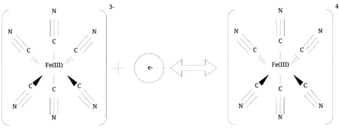
TEC cells work in the following manner: the electrolyte within the cell undergoes a thermally driven oxidation/reduction reaction that results in power generation at electrode surfaces. There are two types of TEC cells one with a stationary electrolyte (sTEC cell) fig. 1-1, and one with a flowing electrolyte (fTEC cell) fig. 1-2. Both operate under the same principle of thermally driven oxidation/reduction reactions. The specific electrolyte I used for this thesis was an equimolar so-lution of a Fe(CN)6 3--/Fe(CN) 64 redox couple where the thermodynamics and electrodynamics

follow the reversible redox chemical reaction:

L N N N N N N C C \C C /Fe(III)- e- FORDI) N N

Figure 2-2: The transition-metal complex of an Fe3+ ion bounded to six CN- ligands that reduce (gain an electron) to create another transition-metal complex of Fe2+ bounded to six CN- ligands, all in an octahedral geometry.

2.3.1 Electrodynamics

We first turn our attention to the molecular level in our study of the Fe(CN)6

3-

4-redox system so that we may better understand electron movement. These ions initially start out as potassium salts which were dissolved in deionized water. What is left in the beaker upon the dissolution of these salts are transition-metal complexes, namely an Fe2+/3+ ion surrounded by CN ligands in an octahedral geometry [9], fig. 2-2.

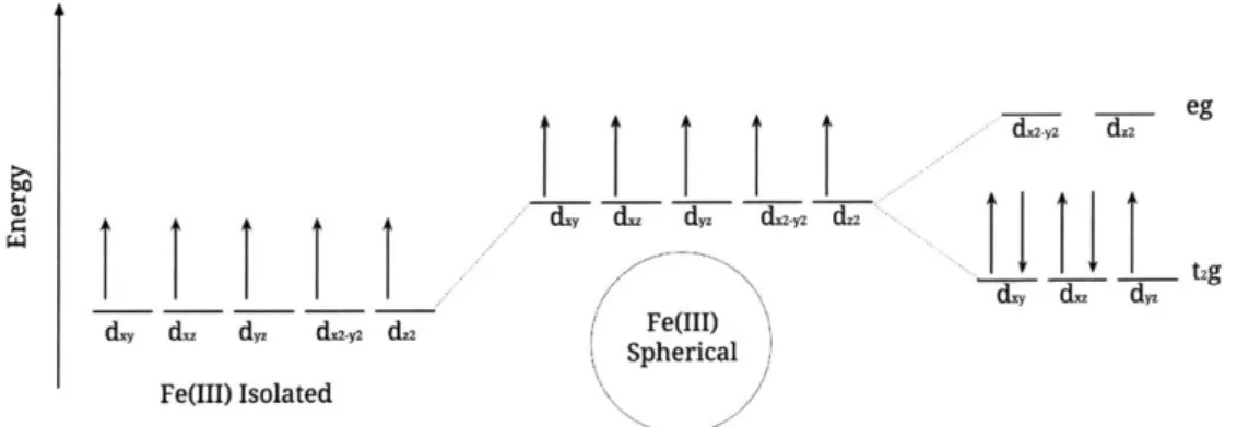
When the oxidation/reduction reaction takes place, the electron moves into one of the five d-orbitals of the Fe3+ ion, turning it into an Fe2+ ion. Crystal field theory [9] gives us a picture as to the location of this new electron, fig. 2-3. Fe3+ binded to six CN- ligands, gets reduced in a half-reaction at the first electrode to Fe2+ binded to six CN- ligands. Fe3+ is a d5 system with five electrons in its d-orbital. The Fe3+ ion receives an electron into its t2g d-orbital to become Fe2+. This is a favorable galvanic cell reaction, because the redox potential is positive and as a result the reaction is spontaneous in the forward direction, i.e. its Gibbs free energy AG is negative in the forward direction: Ej > 0 (2.7) AGO = -nFE < 0 (2.8) = -- 34.35 kJ/mol, (2.9) 0

1-i 1-i

r

ieg

dy da dy,

d.y d. dy. & d. Fe(III)

Spherical Fe(III) Isolated

Figure 2-3: A crystal field theory energy diagram for the five d-orbitals of the Fe3+ ion. The incoming electron will be placed in the dyz orbital since electrons want to occupy the lowest energy state available.

where n = 1 is the number of electrons transferred in the reaction, and F = 96485 C/mol is Faraday's constant.

Now that we have a pretty clear picture of the forward reaction, we must consider the back-wards reaction, i.e. the oxidation half-reaction of Fe2+ back to Fe3+, where an electron is liberated from the t2g d-orbital and transferred to an external circuit. This is not a favorable reaction under standard conditions since the backwards reaction has a negative reduction potential, E0 <0. This implies that the reaction is not spontaneous in the backward direction, i.e. AGO = -AGO

>

[Fe(CN)3-]

AGb= AGO + RT ln _e. (2.10)

b b _[Fe(CN)4-]

In fact we can raise the temperature just enough to thermally regenerate Fe(CN)3~ from Fe(CN)--, by making the backwards reaction spontaneous, i.e. making AGb < 0. After the forward reaction occurs then we are left with an overabundance of [Fe(CN)4-] and almost no

[Fe(CN)--]. This is enough to make AGb < 0.

This allows us to continually oxidize and reduce the Fe2+/3+ ions within the fluid, allowing for continual transport and flow of electrons to an external circuit.

cell under a prescribed temperature difference between two electrodes, ASrX RT [Fe(CN) --] E E (Tb - TO) + In (2.11) nF nF [Fe(CN)4-] S RT [Fe(CN) -] Ef - EO =(Tf - TO) + -In 6(2.12) f TnF _{nF [Fe(CN)}

_/-]

As seen, in order to maximize the voltage output we either increase the temperature difference between the anode and the cathode or select a material with a higher Seebeck coefficient Se =

ASrx nF

I specifically chose Fe(CN)63-/ Fe(CN)64- as the oxidation/reduction system due to its high

Seebeck Coefficient of ~1.4-1.6 mV/K [13, 21, 17]. This results in a high open-circuit voltage.

Voltage output alone does not paint a complete picture of the system. Power generation is a function of both current and voltage output, and a high power output requires a high voltage and high current output. Current output can be thought of as electron fluxes at the electrodes, both anode and cathode. Fluxes at electrode surfaces result in a buildup of current densities that are determined by the kinetics of the chemical reactions at the electrode i, i E

{anode,

ji

I

where the n is the number of electrons transferred in the reaction, F is Faraday's constant, KO is the reaction rate constant, Ex, is the activation energy for the reaction, R is the ideal gas con-stant, To is the reference temperature, T is the temperature at the ith electrode, 0 is a constant determined by the reversibility of the reaction, j is the overpotential generated by the reaction at the ith electrode, and C/C is the oxidized/reduced species concentration at the ith electrode.

With the current output and voltage output, we can now determine the power output:

Experimentally, however, the maximum power output takes the form [14]:

Pmax = 0.25VocIsc, (2.16)

where Voc is the open-circuit voltage and Ic is the short-circuit current.

As mentioned previously, the mass flow of the electrolyte is beneficial, as it would aid in move-ment of ions. For a typical sTEC cells, ion transport from the anode to the cathode is restricted to natural convection, diffusion and migration. However, in the fTEC cell the forced convection of ions replenishes and removes any already oxidized or reduced ion species at the electrode surface. Unidirectional flow restricts movement of ions backwards and reduces one of the performance-limiting steps in fTEC cells, that of ion transport, to and from electrode surfaces.

2.3.2 Heat Transfer & Fluid Mechanics

We can model the fluid mechanics and heat transfer of the electrolyte using a steady state mo-mentum conservation of a laminar flow with only gravitational forces present. Assuming a no slip condition at the wall (U'iewai = 0) we get that

(U -V)iI=vV2 -

+

Po/

where U' is the velocity field of the fluid, p the density of the fluid, V the viscosity of the fluid, and g gravity. This equation is used in our computational model, and interacts with a thermal module to determine the temperature and velocity field of a flowing electrolyte.

The fluid, in our system, convects heat from the constant temperature heat source. The tem-perature of our fluid therefore is defined by the unsteady heat conduction equation:

aT

at = V - (k VT) - p cpV - (U-T) +

Q

U = (u,v) (2.19)

Q = (0, 0) , (2.20)

where k is the thermal conductivity of the fluid, T the temperature of the fluid, and

Q

The flow is assumed to be laminar and incompressible, i.e. divergence free (V - U = 0), with a known velocity profile and a uniform, constant thermal conductivity (V - k = 0). We also seek a steady state solution where D = 0. With these assumptions we get that

p cp 17 - (U T) = p cp (T 17 . U

+

= V - (kVT) + Q (2.22)

= (V - k) VT + kV2_{T+Q (2.23)}

'Ihe steady state solution for the temperature distribution, which will assist in understanding the power output as a function of the fluid velocity U- is given below:

pcPEV - T = kV2T+Q (2.24)

To better pose the above problem, I compared the convection of heat to that of diffusion of heat. Convection occurs in the flow direction and diffusion occurs in the transverse direction. 'The Peclet gives the ratio of advection of temperature to diffusion of temperature. Since our problem is two-dimensional, the Peclet number must be calculated twice; advection will dominate one dimension and diffusion will dominate the other:

Pe = ~

L (2.25)

k

Pey = k << 1. (2.26)

In the flow direction the convection and diffusive of heat are of a similar order whereas in the non-flow direction, the diffusive terms dominates. As a result, we will make a simplifying assumption that advection dominates diffusion, in the flow direction.

Of equal interest to us is the heat transfer coefficient of the fTEC cell as a function of flow rate. Since an fTEC cell can be modeled as a heat exchanger with a constant temperature boundary condition, the heat transfer coefficient can be found by

-MrCP _ATin

h = ln (2.27)

where ri is the mass flow rate of the fluid, w -h is the cross sectional area perpendicular to the flow

direction, cp is the heat capacity of the electrolyte,

A

These equations are solved in the COMSOL model to perform the numerical analysis in chap-ter 4.

Chapter 3

Device Fabrication & Experimental

Setup

In this chapter we review the design of the fTEC cell, the iterations that the design went through, the fabrication of the device, and the experimental setup.

3.1 Design & Fabrication of the Cell

Prior to fabricating the fTEC cell I first identified that the fTEC cell must follow certain require-ments: the cell must be

- leak free,

- thermally conductive,

* compatible with Fe(CN)₆3 _/Fe(CN)

64- electrolyte,

* capable of in-flow electrode insertion,

" electrically isolating.

In the first iteration of the cell, I was aware of all of the design requirements except for the last one, a flaw in iteration one & two which will be discussed more in section 4.2.

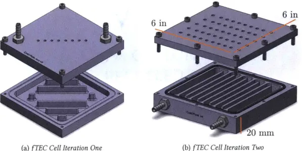
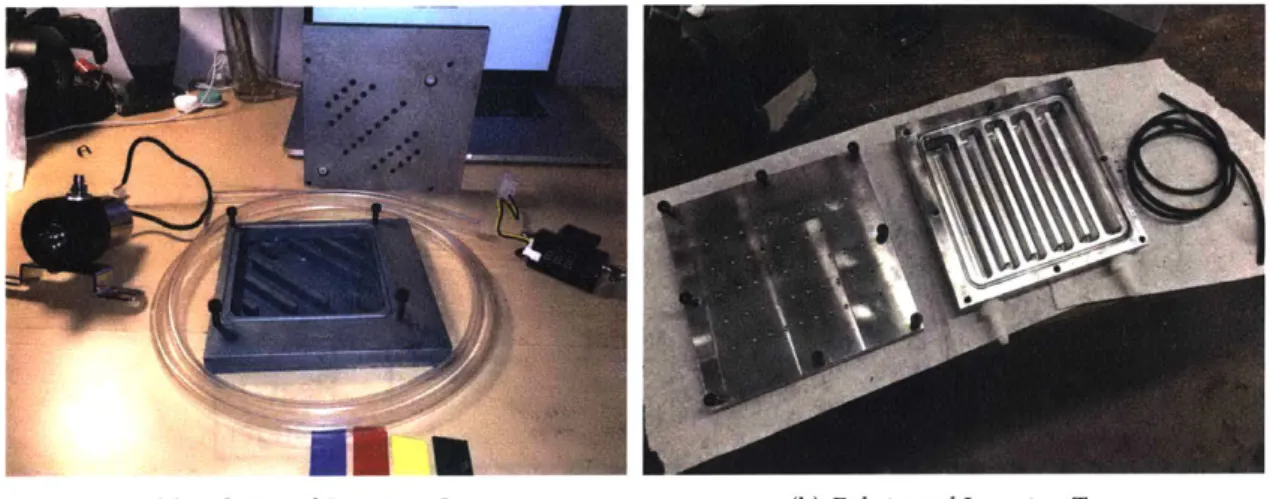
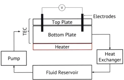
For both iteration one & two I used Solidworks & MasterCam to design and create the G-Code for CNC machining. I used the Prototrak Mill in MIT's Hobby shop to machine two iterations of this device out of 6061-T6 aluminum. The designs can be seen in fig. 3-1a & 3-1b.

3.1.1 Iteration One

Prior to iteration one of the fTEC cell, I had never done any hardcore CNC machining myself. As such, iteration one can be broken down into two sub-iterations called non-working and working. The design of iteration one was inspired by common liquid cooling blocks that are mounted to CPU units. These units are marked by a high surface area geometry and high thermal con-ductivity materials, typically copper. The high surface area allows for more liquid to solid points of heat exchange while the high thermal conductivity of the material assists in transferring heat readily to those points from the heat source. The reason for following this design paradigm is be-cause the fTEC I was designing has an application in the space of CPU cooling whereby the heat released from the CPU chip drives the oxidation reduction/reaction at the electrodes within the fTEC electrolyte thereby generating electricity.

Iteration one has the following design features that were intended to make experimentation simple: NPT tapped holes on the top for electrolyte inlet/outline lines, holes in the top plate along the flow path to allow for easy insertion of graphite electrodes, and a sealing rim around the cell that was filled with sealant to prevent leaks. The machined iteration one can be seen in fig. 3-3a. The material is 6061-T6 aluminum a metal that is compatible (unaffected by the corrosive nature of the electrolyte) with the working fluid.

Takeaways from Iteration One

Iteration one has too many variable dimensions and sizes for it to be of any use in scientific in-quiry. The spacing between the "channels" was not uniform, and the electrode placements were not consistent. Secondly, the sealing rim did not seal properly resulting in many leaks. With the variable sizes, it was impossible to predict what my flow regime would look like, i.e. is each chan-nel experiencing laminar flow, where I can predict the flow profile with a parabola? This would allow me to better estimate heat transfer within the cell if I were to have this knowledge; hence I made those improvements in iteration two.

(a) fTEC Cell Iteration One

6 in6in

20 mm

(b)

fT

Figure 3-1: The two iterations of the fTEC cell. From the first iteration of the cell (a) I made design modifications, such as a snaking fluid path, side inlet/outlet holes, and inline electrode holes so that iteration two (b) would provide a more accurate (and cleaner a.k.a. leakproof) function of the cell.

3.1.2 Iteration Two

Iteration two built upon the takeaways from iteration one. I designed the channels to be of constant width, the electrode hole locations to be in a "matrix" form for variable electrode distance testing, and the inlet/outlet lines placed on the side of the cell. The machined iteration two can be seen in fig. 3-3b. 'The issues that arose with iteration two are quite different than those from iteration one and only arose due to testing the experimental setup.

For each hole in the top plate of the cell, I needed to insert both a thermocouple and a graphite electrode (for reasons that are discussed in section 3.3). Ensuring that I could insert both the electrode and the thermocouple, while also ensuring that the device was leakproof during oper-ation, was a beast of its own. Initially, I attempted to wrap both the thermocouple and graphite electrode in heatshrink tubing to create a compliant seal when inserted into the top plate. This did not prevent any leaks. To combat this, I spread RTV gasket sealer all over the electrode hole but nonetheless leaks persisted.

After dealing with the leaking issue for a while, I finally stumbled across a chemically resistant nylon multi-cord grip, fig. 3-2. One end of the cord-grip is NPT threaded so that I could NPT tap into the top plate and use teflon tape to create a seal. This solution worked well.

Figure 3-2: The multi-cord nylon seal with NPT thread was threaded into the top plate to prevent leaks for the electrode and thermocouple probes.

3.2

Electrolyte Preparation

The working fluid for my experiments was an equimolar solution of Fe(CN)63-/Fe(CN)64-. At

0.4 M, the solution is at its highest possible redox couple concentration, but still low enough to avoid electrolyte degradation at high concentrations [15], allowing me to maximize the kinetics of the chemical reaction, resulting in an increased current output.

Since I desired a 0.4 M solution, utilizing a 750 mL container, I needed 0.3 moles of total solute. The solution should be equimolar K3(FeCN)6 = 329.24 g/mol and K4(FeCN)6 = 422.39 g/mol,

therefore we need 0.15 moles of each solute. This results in a mass of K3(FeCN)6 = 49.39 g and a

mass of K4(FeCN)6 = 63.36 g to be dissolved in a 750mL container of deionized water to create

a 0.4 M solution.

3.3

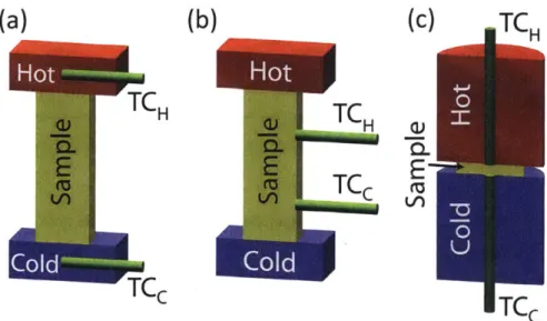
Experimental Setup

The purpose of these experiments was to determine how the fTEC cell functions, i.e. what is its power/voltage/current outputs and heat trasnfer coefficient, at different flow rates. Fig. 3-4 shows a global diagram for the experimental setup that guided the physical setup for the experi-ment. Fluid is pumped from a resevoir, into the fTEC cell where it is heated. The heat drives an oxidation reduction reaction at the electrodes thereby generating electricity. Then the fluid leaves the fTEC cell and cycles back into the reservoir. For these experiments, a closed-loop fluid system was desirable for easy operation and testing. The difference between a closed-loop and open-loop

I

~59~

Eta

(a) Fabricated Iteration One (b) Fabricated Iteration Two

Figure 3-3: The two iterations of the fTEC cell after they have been machined. The main differ-ence between iteration one (a) and iteration two (b) are a longer flow path, smaller channels, and variable 2D electrode placement.

fluidic system is that in the closed loop, the fluid passes through the fTEC cell (after having un-dergone an increase in temperature) and then has its excess heat dissipated through an external heat exchanger before returning to the fluid reservoir.

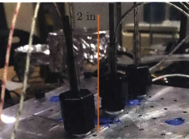
The main parameters of interest in the system are the flow rate, the temperature of the fluid at the electrodes, and the voltage/current output at the electrodes for a given electrode distance. To set the flow rate, I used a Cole-Parmer peristaltic pump. I used in-line K-type thermocouples at the electrode locations and a temperature probe in the reservoir bath to monitor fluid inlet temperature and temperature at the electrodes. The voltage and current outputs were measured using a potentiostat.

The purpose of each experiment was to determine the tempererature difference, heat transfer coefficient, open-circuit voltage, and current output between two in-line electrodes, as a function of flow rate. This will allow me to determine the power generation capabilities of the fTEC cell as well as its effectivness at heat removal from a heat source. For each experiment, I ensured that the the heater was at a constant temperature of 400 K and I let the peristaltic pump run for some time until the fluid reached a steady-state outlet temperature. Experimentally, the steady-state point was characterized by no temperature increase of the fluid after two minutes of operation. This op-eration only needed to be performed once per testing "session.' Two itop-erations of my experimental setup can be seen in fig. 3-5a & 3-5b.

V

ELectrodes

Top Plate

Bottom PLate

Heater

Heat

Pump

_Exchanger

Fluid Reservoir

Figure 3-4: A schematic of the experimental setup. Electrolyte gets pumped to the fTEC cell by a peristaltic pump, the heater heats the electrolyte which consequently reacts at the electrode surfaces, generating a voltage. The system is closed loop, with the fluid resevoir maintained at a constant temperature.

Once steady-state was reached, I turned on the potentiostat and ran two methods: an open-circuit voltage method, and a chronoamperometry method. The open-open-circuit voltage method would measure the open-circuit voltage for three minutes, which should correspond to the temper-ature difference I recorded by a handheld thermocouple meter multiplied by the Seebeck coefficient of the electrolyte. The second method I ran was a chronoamperometry method which logged the short-circuit current over time. With the open-circuit voltage Vc and the short-circuit current Isc, I was able to calculate the maximum experimental power of the device by

Pmax = 0.25 IscVoc. (3.1)

With regard to material selection, it is important to note that the corrosiveness of the elec-trolyte was a limiting factor. The chemical compatibility between the elecelec-trolyte and 6061-T6 aluminum proved to be moderate and suitable for this experiment. All connectors are NPT with chemically inert rubber tubing connecting the components of the system.

(a) Experimental Setup Iteration One (b) Experimental Setup Iteration Two

Figure 3-5: The two iterations of the experimental setup for the fTEC Cell. The main difference between iteration one (a) and iteration two (b) are that the second iteration paid more careful attention to monitoring all variables in the system, one example is having a constant temperature bath for the inlet electrolyte.

3.3.1

Electrode Selection

For the electrode material, I utilized extruded graphite. Studies have been conducted on different electrode materials, such as carbon nanotubes for their high surface area. Graphite was chosen as the electrode material for its thermodynamic stability [11]. The electrodes were inserted into the top plate of the device, electrically isolated from the cell, and connected to a potentiostat.

Chapter 4

Device Performance

The fTEC cell that I built was characterized by its ability to convect heat and its ability to generate power. These two properties of the cell are at odds with each other, since at lower flow rates I observed a higher power output but a lower heat transfer coefficient but for a higher flow rate, I observed a lower power output and a higher heat transfer coefficient. In order to validate these ob-servations I evaluated the fTEC cell using numerical simulations and experiments. The numerical simulations were performed with COMSOL.

4.1

Numerical Analysis

The COMSOL analysis of the fTEC cell involved creating a two dimensional domain and then solving the multiphysics equations specified in section 2.3.

4.1.1 Domain Setup

I wanted to simplify my three dimensional fTEC cell to a tractable two dimensional system for numerical analysis. To this end, I decided to take a "differential" element of my fTEC cell, i.e. a side view of the flow channel bounded on each end, spatially, by two electrodes. The domain can be seen in fig. 4-1. The electrolyte enters from the left hand side of the element, is exposed to a constant temperature boundary condition, undergoes thermally driven oxidation/reduction reactions and then exits the cell on the left side.

0.02 0.018 0.016 0.014 0.012 0.01 -40 0.008 0.006 0.004 0.002 C -0.005 0 0.005 0.01 0.015 0.02 0.025 0.C

Figure 4-1: The "differential" domain for my numerical analysis. The electrolyte flows in from the left, into the element, is exposed to a constant temperature boundary condition, oxidizes and reduces at the electrodes, and then exits the element.

solve the multiphysics problem. I sought a steady-state solution to the problem: electrolyte enters the left side of the element at equimolar concentrations, the ions reduce at the first electrode, un-dergo a temperature increase by the constant temperature boundary condition, and then oxidizes at the outlet electrode.

Specifically, the assumptions and geometry of the model are as follows:

- the cell measures 2.54 cm x 2 cm,

- the inlet volumetric flow rate of the electrolyte ranged from 10 GPD to 100 GPD,

* the boundary condition on the cell is a constant temperature boundary conditions of 400 K,

- the left and right edges of the boundary are set to be the electrode locations,

" the inlet temperature of the fluid was room temperature at 293.15 K,

" and fully devleoped (thermally and hydrodynamically) laminar flow.

With this model, I was able to predict voltage, current, and power output with respect to flow rate. I was also able to predict the heat transfer coefficient of the cell.

A 400A 0.05 0.024 -A40 0.024 XI-I 0.022 0.02245 0.0 390 0.02 0.01 380 0.018 4 0.013 0.016 -370 3.5 0.01 0.014 360 0.012 0.00 0.02 - 0.0 2.5 0.00 ' 0.008 340 o.004 0.006 0.004 3 0.004 , , ,,a s s , - . , .- . . . 1.5 0.002 -320 0.002 310 -0.002 30 -0,002 0.5 -0.004 30 -0.004 0.005 0.01 0.015 0.02 0.005 0.01 0.015 0.020 Distance between Electrodes (m 2 V 293 Distance between Electrodes (m) V 0

(a) Temperature Profile (b) Velocity Profile

Figure 4-2: (a) The steady state fully developed two dimensional temperature profile within the electrolyte under a constant temperature boundary condition. (b) The steady state

lfully

4.1.2 Results

The constant temperature boundary condition is the driver of the chemical reaction at the trodes. Numerically, we can see the two-dimensional temperature distribution in a flowing elec-trolyte at steady-state, as well as the velocity profile of the elecelec-trolyte at steady-state in fig. 4-2a & 4-2b. The electrolyte obtains a maximum temperature increase to approximately the tempera-ture of the boundary, while temperatempera-ture diffuses inward. Clearly, the electrolyte has a parabolic velocity profile of the non-dimensional form:

i(y)= I - (4.1)

where y is the distance from the centerline of the "differential" element, and h is the total height of the element. We should note that the heat flux imposed by the constant temperature boundary condition does not diffuse that far into the element itself.

2.2 320 2 300 1.8 280 1.6 _E 260 1.4 240 1.2 220 200 4) 180 0.6 -160 0.4-140 0.2 120 10 20 30 40 50 60 70 s0 90 100 10 20 30 40 50 R ( 70 80 90 100 Flow Rate GP)Flow Rate (8 PD)

(a) Inlet/outlet temperature difference vs. Flowrate (b) Heat Transfer Coefficient v. Flowrate

Figure 4-3: (a) The inlet/outlet temperature difference as a function of the flow rate. As we expect, the difference decays exponentially as the flow rate increases. (b) The heat transfer coefficient as a function of flow rate. As expected, we see a higher heat transfer coefficient with increasing flow rate.

Power Generation

With the knowledge of the temperature distribution of the fluid, we can readily calculate how the inlet/outlet temperature difference varies with the flow rate. I had many options as to what spatial coordinate I would select to evaluate the temperature. I selected the midline of the "differential" element as the point to evaluate inlet and outlet temperature since this is the point, within my experiments, to which my electrodes reach when embedded in the top plate of the fTEC cell. As we can see in fig. 4-3a the maximum temperature difference of the inlet and outlet of the fluid is AT = 2.2 K. Since the electrolyte I was using has a Seebeck coefficient of Se = 1.5 mV/K then we expect that the maximum Vc = ATSe = 3.3 mV. The Vc as a function of flow rate is plotted in fig. 4-4a. As the flow velocity increases the temperature at the inlet and outlet will decrease. Therefore since the voltage output is proportional to the difference in inlet/outlet temperature, we expect the voltage output to decrease with increasing flow rate.

I also determined the short-circuit current as a function of the flow rate. Its trend follows a similar decay as the open-circuit voltage. As the flow rate increases, there is less time for each ion

45 2.55 44.5 2.8 44 2.5 2.6 2.4 42 2.2 43 2,45 1 42.5 1.4 1.2 41.5 2.35 40.5 2.3-:A 0.4 40 10 20 30 40 S 64 70 8 90 144 10 20 30 40 FO5 ( ) 70 84 90 100 10 20 30 44 F ( ) 70 80 90 100 F14.45(P2 Rate48M87)p F1448 X I

(a) Voltage vs. Flowrate (b) Current vs. Flowrate (c) Power vs. Flowrate

Figure 4-4: (a) The voltage output of the cell decreases as flow rate increases, indicative of a lower temperature difference between the inlet and the outlet. (b) The current output of the cell decreases as flow rate increases, indicative of less time for ions to interact with the electrode surfaces and exchange electrons. (c) The power output of the fTEC cell as a function of flow rate. The maxumim power output I numerically observed was Pmax = 2.55 pW

to interact with the electrodes and transfer electrons to an external circuit. As a result, we expect the current to decrease with increasing flow rate. The behavior can be seen in fig. 4-4b. Now knowing both voltage and current I can determine the power output of the cell as a function of the flow rate. The maxumim power output I numerically observed was Pmax = 2.55 PW, as seen in fig. 4-4c.

Heat Transfer

The heat transfer coefficient is a good metric to evaluate the effectivness of the fTEC cell as a heat exchanger. With a constant temperature boundary condition, and knowledge of the inlet/outlet temperatures and the boundary condition temperature, we can use eq. 2.27 to calculate the heat transfer coefficient. The heat transfer coefficient as a function of flow rate is plotted in fig. 4-3b. Clearly as the flow rate increases, the heat transfer coefficient increases, thus confirming our observation that power generation and heat transfer capabilties are at odds with each other. Numerically we observe a maximum heat transfer coefficient of approximately 340 W/m2K.

This numerical analysis served as a solid basis on which I could evaluate (and validate) my physical fTEC cell, by comparing these results to my experimental results.

2 20 S15 -10 C C 0 5 0 50 100 150 200 0 50 100 150 200 Time (s) Time (s) 80 -60 C60 40 40 2 0 0 Ca- 20 _{a- 0} 0 -0 50 100 150 200 0 50 100 150 200 Time (s) Time (s)

Figure 4-5: The first set of experiments where I recorded the voltage, current, and power outputs of the fTEC cell versus time. I recorded a AT = 2 K which corresponds correctly to a voltage output

of Vc = 3 mV. However, the current and power outputs do not correspond well to the values I acheived numerically. 'Ihis meant that something was wrong with my experimental setup.

4.2 Experimental Results

I experimentally determined the voltage, current, and power outputs for the fTEC cell as a function of the flow rate. I also determined the heat transfer coefficient of the fTEC cell for different flow rates. I first tested the cell using deionized water to ensure that all outputs were zero. After doing

so I embarked on my first set of experiments.

For consistency between my numerical and physical experiments, I evaluated these tempera-ture and electrical outputs of the fTEC cell only between two adjacent electrodes. Following the procedure outlined in chapter 3, I captured all of my electrical output data using a potentiostat, and the temperature data using a hand held thermocouple meter.

The first set of experiments were quite inconsistent. Between two electrodes I recorded a AT =

2 K and a voltage, power, and current output that corresponds to fig. 4-5. Clearly the voltage

output corresponds well to Vc = ATSe, but the current and power outputs do not correspond

well. This informed me that there was something wrong with my experimental setup. At this point in the project I started a collaboration with a 4 th PhD sutdent at Georgia Tech, Ali Kazim who is

one of Professor Baratunde Cola's students, who developed a similar setup to mine. Note here that all data obtained and analyzed by Kazim is owned by him and I am simply referencing his

450 400-E 350-I-C 300 250 20 30 40 50 60 70 80 90 100 Flow rate (gpd)

Figure 4-6: The heat transfer coefficient of the differential element as a function of the flow rate, obtained by Kazim. As we see, as the the flow rate increases, the heat transfer coefficient increases, indicating a greater ability to convect heat from a source.

results for this work. Both of our setups can be seen in fig. 4-7 & 3-3b. After a long discussion we determined that the reason for the erroneous outputs was due to the fact that my fTEC cell was not anodized. The process of anodization creates a thin non-conductive oxide layer on the aluminum thereby removing the possibility for the cell to short-circuit. Without this thin non-conductive layer, the cell would develop a short-circuit whereby the electrons transferred by the ions prefer a path of least resistance which is found simply by entering into any part of the aluminum cell. This is not the behavior that I wanted, especially when measuring the short-circuit current. I wanted the electrons to travel into the graphite electrodes and into the potentiostat for measurement.

Kazim had his fTEC cell anodized and he ran the same experiments and we were able to obtain the following outputs of the cell, fig. 4-8. Kazim was able to also test how different molarities of the electrolyte affected the voltage, current, and power outputs. From this second set of experi-mentation, we determined that the maximum Vc = 16 mV, I, = 50 -10-5 A, and Pmax = 2.0 MW He also determined that different molarities of the electrolyte only affected the current output since a higher molarity implies that there is a higher amount of ions that are readily available to transfer electrons to the electrode surfaces.

The experimentally determined heat transfer coefficient is shown in fig. 4-6. We note that the highest heat transfer coefficient measured was approximately 450 W/m2K.

Rtservoir

Figure 4-7: Kazim's setup for the fTEC cell, using a setup similar to my setup.

a 16 14 -12 8 . 8 6 4 20 30 40 50 60 70 Flow rate (gpd) 80 90 100 b ₅₀ -40 -30 20 10 -2 I I I I I 0 30 40 C 2.0 1.5 E1.0 0.5 0.0 I I I I . I I I ' I 1 1 50 60 70 80 90 100 Flow rate (gpd) - U -7 50 60 70 80i90 100 50 a 70 90 1 Flow rate (gpd)

Figure 4-8: Results obtained using Kazim's setup, we can see a clear decay in the (a) voltage, (b) current, and (c) power output as the flow rate increases.

E7

4.3

Discussion

In general, the numerical results for the "differential" element of the fTEC cell agree quite well with the experimental results. The difference for the maximum voltage, current, and power output is 12.6 mV, 7.10-5 A, and 0.55 pW between the experimental results and the numerical results, and 100 W/m2K for the heat transfer coefficient. For the voltage outputs, I can clearly see that the temperature dictates the voltage output and that at a higher temperature there is a higher voltage output. For the numerical results, however, I observe a lower voltage output for the given geometry than I see for the experimental voltage output. I believe this is the case since the electrolyte in the experimental cell is not guaranteed to undergo laminar flow, if there is any mixing or turbulence then there is a definite higher heat transfer coefficient and consequent temperature difference between electrodes. Secondly, in the actual fTEC cell, voltage is built up along entire surface of the electrode whereas within the numerical domain, the voltage is calculated at a point. However, the exponential decay is consistent between experimental and numerical results. The current and power values are quite similar and attain maximal values at low flow rates. The heat transfer coefficient, both numerically and experimentally, follow a similar trend as a function of flow rate both within the same order of magnitude of each other. A similar argument can be applied to understand the discrepancy between the two heat transfer coefficient values: the unknown nature of the flow regime for the experimental setup. All told, these results are suggestive that the device has been properly tested experimentally and evaluted numerically.