Efficient coding of information: Huffman coding

(1)

GENERAL I ARTICLE

Efficient Coding of Information: Huffman Coding

Deepak Sridhara

In his classic p a p e r o f 1948, C l a u d e S h a n n o n c o n - s i d e r e d t h e p r o b l e m o f e f f i c i e n t l y d e s c r i b i n g a s o u r c e t h a t o u t p u t s a s e q u e n c e o f s y m b o l s , e a c h a s s o c i a t e d w i t h a p r o b a b i l i t y o f o c c u r r e n c e , a n d p r o v i d e d t h e t h e o r e t i c a l l i m i t s o f a c h i e v a b l e p e r - f o r m a n c e . In 1 9 5 1 , D a v i d H u f f m a n p r e s e n t e d a t e c h n i q u e t h a t a t t a i n s t h i s p e r f o r m a n c e . T h i s ar- t i c l e is a b r i e f o v e r v i e w o f s o m e o f t h e i r r e s u l t s . 1. I n t r o d u c t i o n

Shannon's landmark paper 'A Mathematical Theory of Communication' [1] laid the foundation for communication and information theory as they are perceived to- day. In [1], Shannon considers two particular problems: one of efficiently describing a source that outputs a sequence of symbols each occurring with some probability of occurrence, and the other of adding redundancy to a stream of equally-likely symbols so as to recover the original stream in the event of errors. The for- mer is known as the

source-coding

or data-compression problem and the latter is known as the

channel-coding

or error-control-coding problem. Shannon provided the theoretical limits of coding achievable in both situations, and in fact, he was also the first to quantify what is meant by the "information" content of a source as described here.

Deepak Sr/dhara worked as a research associate in

the Deparment of Mathematics at l l S c between January and December 2004. Since January 2005, he has been

a post-doctoral research associate in the Institute

for Mathematics at Unviersity o f Zurich. His research interests include coding theory, codes over

graphs and iterative techniques, and informa-

tion theory.

This article presents a brief overview of the source-coding problem and two well-known algorithms that were dis- covered subsequently after [1] that come close to solv- ing this problem. Of particular note is Huffman's algorithm that turns out to be an optimal method to represent a source under certain conditions. To state the problem formally: Suppose a source U outputs symbols

Keywords

Entropy, source coding, Huff- man coding.

(2)

GENERAL J ARTICLE

1 By a D-ary siring w e m e a n a sequence (YvY2 ... Yn) where each yj belongs to the set {0,1,2,...,D-1}.

Intuitively, the optimal number of bits needed to represent a source symbol uj with probability of occurrence p; is around log 2

llpi

bits.

problem formally: Suppose a source U o u t p u t s symbols Ul, u 2 , . . . , uK, belonging to some discrete a l p h a b e t / ~ , with probabilities

p(ul),P(U2),...,p(ug),

respectively. T h e source-coding problem is one of finding a m a p p i n g from /4 to a sequence of D - a r y strings 1, called codewords, such t h a t this m a p p i n g is invertible. For t h e coding to be efficient, the aim is to find an invertible m a p p i n g (or, a code) t h a t has t h e smallest possible average codeword-length (or, code-length). By t h e way this problem is stated, a source U can also be t r e a t e d as a discrete r a n d o m variable U t h a t takes values from /4 -- {ul, u 2 , . . . ,

uN}

and t h a t has a probability distribution given by

p(V),

where

p(U = ui) = p(ui),

for i = 1 , 2 , . . . , K .

As an example, suppose a r a n d o m variable U takes on four possible values ul, u2, u3, u4 with probability of occurrences

R(Ul)= 1, p(u2)-- 88 P(U3)=

1, p(u4)-~ 1.

A naive solution for representing t h e symbols u l , . . . , u4 in terms of binary digits is to represent each symbol using two bits: ul = 00, u2 = 01, u3 -- 10, u4 = 11. The average code-length in this representation is two bits. However, this representation turns out to be a sub-optimal one. An efficient representation uses fewer bits to represent symbols occurring with a higher probability and more bits to represent symbols occurring with a lower probability. An optimal representation for this example is ul = 0, u2 = 10, u3 = l l 0 , ua = 111. T h e average code-length in this representation is 1- 7 + 2 . ~ + 3 . ~ + 3 . g l 1 1 = 1.75 bits. Intuitively, t h e optimal n u m b e r of bits needed to represent a source symbol ui with probability of occurrence

Pi

is around log 2 ~ bits. Further, since ui occurs with probability pi, t h e effec-

i Shan- tive code-length of

ui

in such a code is

Pi

log2 p'7"

non's idea was to quantify t h e 'information' content of a source or r a n d o m variable U in precisely these terms. Shannon defined t h e

entropy

of a source U to measure its information content, or equivalently, the entropy of

(3)

GENERAL J ARTICLE

a random variable U to measure its 'uncertainty', as

H(U) = ~iPi

log2 ~ The coding techniques discussed

Pi"

in this article are evaluated using this measure of 'information' content.

This article is organized as follows. Section 2 introduces some definitions and notation that will be used in this paper. Section 3 provides the notion of typical sequences that occur when a sequence of independent and identically distributed random variables are considered. This section also states the properties of typical sequences which are used to prove the

achievability

part of Shan- non's source-coding theorem, in Section 4. Section 5 introduces the notion of D-ary trees to illustrate the encoding of a source into sequences of D-ary alphabets. Another version of the source-coding theorem for the special case of prefix-free codes is presented here. A coding technique, credited to Shannon and Fano, which is a natural outcome of the proof of the source-coding theorem stated in Section 5, is also presented. Sec- tion 6 presents Huffman's optimal coding algorithm that achieves a lower average code-length than the Shannon- Fano algorithm. The paper is concluded in Section 7. 2. P r e l i m i n a r i e s

Shannon defined the

entropy

of a source U to measure its information content, or equivalently, the entropy of a random variable U to measure its 'uncertainty', as H(U)=Z,p, log 2

llpr

Some basic definitions and notation that will be used in this article are introduced here.

Let X be a discrete random variable taking values in a finite alphabet A'. For each x E A' let

p(x)

denote the probability that the random variable X takes the value x written as

Pr(X = x).

Definition

2.1. The expectation of a function

f ( X )

de-

fined over the random variable X is defined by

E[f(X)] = ~ f(x)p(x)

xE)~

Definition

2.2. The entropy

H(X)

of a discrete random

(4)

GENERAL [ ARTICLE The entropy H(X) of a discrete random variable X is defined by H(X) = - Z p(x) log p(x). XE,,~" variable X is defined by

H (X) = - ~ p ( x ) logp(x).

xEA'

To avoid ambiguity, the term

p(x)

logp(x) is defined to be 0 when

p(x)

= 0. By the previous definition,

H(X) =

-E[logp(X)].

For most of the discussion, we will use logarithms to the base 2, and therefore, the entropy is measured in bits. (However, when we use logarithms to the base D for some D > 2, the corresponding entropy of X is denoted as

HD(X )

and is measured in terms of D-ary symbols.) Note that in the above expression, the summation is over all possible values x assumed by the random variable X, and

p(x)

denotes the corresponding probability of X = x.

We will use uppercase letters to indicate random variables, lowercase letters to indicate the actual values assumed by the random variables, and script-letters (e.g., X) to indicate alphabet sets. The probability distribution of a random variable X will be denoted by

p(X)

or simply p.

Extending the above definition to two or more random variables, we have

Definition

2.3. The joint entropy of a vector of random variables (X1, X 2 , . . . , Xn) is defined by H ( X 1 , X 2 , . . . , X n ) = - - ~, P ( X l , ' ' ' , X n ) l O g p ( X l , X n . . . , X n ) (zl,x2 ... =,-,)e,Vl xX2x...xX,-, w h e r e p ( x l , x 2 , . . . X n ) = P r ( X 1 = X l , X 2 : x 2 , . . . X n __~

Xn).

Definition

2.4. (a) A collection of random variables {X1, X 2 , . . . X,~} with Xi taking values from an alphabet A" is called independent if for any choice {Xl, x 2 , . . , xn}

(5)

GENERAL I ARTICLE

with X i = xi, i = 1, 2 , . . . n, the probability of the joint event {X 1 = X l , . . . , X,~ = xn} equals the product

n

1-Ii=l P r ( Z i = xi).

(b) A collection of r a n d o m variables {X1, X 2 , . . . Xn} is said to be identically distributed if 2(i = 2(: t h a t is, all t h e alphabets are t h e same, and the probability P r ( X i =

x) is the same for all i.

(c) A collection of r a n d o m variables {X1, X 2 , . . . X , } is said to be i n d e p e n d e n t and identically distributed (i.i.d.) if it is b o t h i n d e p e n d e n t and identically distributed. An i m p o r t a n t consequence of i n d e p e n d e n c e is t h a t if {X1, X2,. 9 9 Xn} are i n d e p e n d e n t r a n d o m variables, each taking on only finitely m a n y values, t h e n for any function f/(.), i = 1 , 2 , . . . n ,

n n

E[ H f i ( X i ) ] = H E [ f i ( X i ) ] .

i = 1 i = l

Thus if {X1, X2,. 9 9 Xn} are i n d e p e n d e n t and take values over finite alphabets, t h e n the entropy

H ( X ] , X 2 , . . . X n ) =- - E [ l o g p ( X 1 , X 2 , . . . X,~)] =

n n

E[logp(X,)] = ~ H(X,).

i = 1 i = l

If, in addition, t h e y are identically distributed, t h e n

A collection of random variables {X,, X 2 ...

X~}

is said to be identically distributed if ~=.r that is, all the alphabets are the same, and the probability

Pr(Xj=x)

is the same for all i.

H ( X I , X 2 , . . . X n ) ---- nH(Xi) = n H ( X l ) .

Note t h a t if X1,. 9 9 Xn are a sequence of i.i.d, r a n d o m variables as above, t h e n their joint entropy is H ( X a , X2,

. . . , X n ) = n H ( X ) .

D e f i n i t i o n 2.5. A sequence {]In} of r a n d o m variables is said to converge to a r a n d o m variable Y in probability if for each e > 0

P r ( I Y n - YI > ~) , O, as n , ~ ,

(6)

The assertion that X . ~ E[X1] with probability one is called the strong law of large numbers and

the assertion that

X,-~ E[X1] in

probability is called the weak law of large

numbers.

56

and

with probability one

if

Pr(

lim Yn = Y) = 1. n - - - * OQ

It can be shown that if Yn converges to Y with probability one, then Yn converges to Y in probability, but the converse is not true in general.

The

law of large numbers

(LLN) of probability theory n

says that the

sample mean Xn -- 1/n ~-],i=1 Xi

of n i.i.d, random variables { X 1 , X 2 , . . . X n } gets close to

m = E[Xi]

as n gets very large. More precisely, it says that ){n converges to

E[Xa]

with probability 1 and hence in probability. Here we are considering only the case when the random variables take on finitely many values. The LLN is valid for random variables taking infinitely many values under some appropriate hypothesis (see R L Karandikar [4]). The assertion t h a t ){n ) E[X1] with probability one is called the

strong law of large numbers

and the assertion that ){,~ )

E[X1]

in probability is called the

weak law of large numbers.

See Karandikar [4] and Feller [5] for extensive discussions (including proofs) on both the weak law and the strong law of large numbers.

3. T y p i c a l S e t s a n d t h e A s y m p t o t i c E q u i p a r t i - t i o n T h e o r e m

As a consequence of the law of large numbers, we have the following result:

Theorem

3.1. If Xa, X 2 , . . . are independent and identically distributed (i.i.d.) random variables with a probability distribution p(.), then

1

- - - l o g p ( X 1 , X 2 , . . . , X n ) ~ H ( X )

n

with probability 1.

Proof.

Since X 1 , . . . , X ~ are i.i.d, random variables,

(7)

p(Xl,... ,X?%) = Hip(X,).

Hence,

l logp(X1,X2, ... ,X?%)

1 Z l o g p ( X i )

n n

i

converges to

-E[logp(X)] - H(X)

with probability 1 as n , oo, by t h e s t r o n g law of large numbers. 9

1

This t h e o r e m says t h a t t h e q u a n t i t y ~ log

p(x;:x2...,x,)

is close to t h e e n t r o p y

H ( X )

w h e n n is large. Therefore, it makes sense to d i v i d e t h e set of sequences (Xl, x2, 9 9 9 x?%) 9 9='?% into two sets: t h e

typical set

wherein each sequence (xl, x 2 , . . 9 xn) is such t h a t 1 l o g 1 is close to the e n t r o p y H ( X ) a n d the non-typical set c o n t a i n i n g 1 log 1 b o u n d e d away from t h e sequences w i t h ~ p(~l ... ~,)

entropy

H(X).

As n increases, the probability of sequences in t h e typical set becomes high.

Definition

3.1. For each e > 0, let A~ 7%) be t h e set of sequences (xl, x 2 , . . . , x?%) 9 9:'?% with the following property:

2 -n(H(X)+e) ~_ p ( x l , x 2 , . . . , x?%) ~ 2 -?%(H(x)-e).

Call A~ 7%) a typical set.

Theorem

3.2. Fix e > 0. For A~ 7%) following hold:

as defined above t h e

. If

(Xl,X2,...,x?%) 9 A~ n),

t h e n

H ( X ) - e < _ z

_?% l o g p ( x l , x 2 , . . . , x ? % )

<_ H(X) + e.

. If {X 1, X 2 , . . . X?%} are i.i.d, with probability dis- t r i b u t i o n

p(X)

t h e n

Pr((xl, x2,...xn) e A! 7%)) -

Pr(A! 7%))

~ 1 as n , c~.

3. JA~?%)J _<

2 n(H(X)+r

w h e r e for any set S, JS I is t h e n u m b e r of e l e m e n t s in S.

4. JA~?%)[ > (1 -

e)2 n(H(X)-~)

for n sufficiently large.

(8)

GENERAL J ARTICLE Shannon's source- coding theorem states that to describe a source by a code C, on an average at least H(X) bits (or, D-ary symbols) are required.

Proof.

The proof of (1) follows from the definition of A! n) and that of (2) from Theorem 3.1.

To prove (3), we observe that the following set of equa- tions hold:

1----

Z

p(Xl'"

"''Xn) ~

Z

P ( X l ' "

"''Xn)

(xl ... z,~)eX" (z ! ... z,~)EA~,~) > (xl ... x,,)eA~ '')

2-n(H(X)+ ~) = 2-n(H(X)+e)JA~n)l.

To prove (4), note by (2) that for n large enough

P r ( ( x l , . . . , x , ) 9 A~ ")) > 1 - e.

This means that

1 - e < P r ( ( x l , . . . , x , ) e A!"))=

p ( x l , x 2 , 9 9 9 x n )

(xl ... x.)eA~ ")

<

4. S o u r c e C o d i n g T h e o r e m

Shannon's source-coding theorem states that to describe a source by a code C, on an average at least

H ( X )

bits (or, D-ary symbols) are required. The theorem further states that there exist codes that have an expected code- length very close to H (X). The following theorem shows the existence of codes with expected code-length close to the source entropy. This theorem can also be called the

achievability-part

of Shannon's source-coding theorem, and says that the average number of bits needed to represent a symbol x from the source is H ( X ) , the entropy of the source.

(9)

GENERAL [ ARTICLE

Rgure 1. Typical sets and source-coding.

Theorem

4.1. Let X n = ( X 1 , X 2 , . . . X n ) be an inde- p e n d e n t and identically distributed (i.i.d.) source w i t h distribution

p(X).

Let t? > 0. T h e n t h e r e exists an n o -- n0(y), d e p e n d i n g on ~ such t h a t for all n > no, there exists a code which m a p s sequences x n = (xl, x 2 , . . . , xn) of length n into binary strings such t h a t the m a p p i n g is one-to-one (and therefore invertible) and

E[lg(xn)] < H(X) 4- rh

where

g(x '~)

is t h e l e n g t h of t h e code representing x n.

Proof.

Let

X1,X2,... ,X,

be i.i.d, r a n d o m variables chosen from t h e probability distribution

p(X).

T h e goal is to find short descriptions for such sequences of ran- d o m variables. Consider t h e following encoding scheme: For a chosen e > 0 a n d integer n > 0 (both to be chosen later) partition t h e sequences in ,l:'n into two sets: t h e typical set A! '~) and its c o m p l e m e n t as shown in

Figure

1. Order all t h e e l e m e n t s in each set according to some order. T h e n we can represent each sequence of A! ~) by giving t h e index of t h a t sequence in the set. From Theo- rem 3.2, there are at m o s t 2 n(H(x)+~) such sequences, and hence, the indexing of elements in A! ") requires no more t h a n

[n(g(x) +

e)] <

n(H(X)

+ e ) + 1 bits. Similarly, the sequences not in A! n) can be indexed by In log 12dl] < n log IX I + 1 bits since t h e n u m b e r of sequences not in the typical set is less t h a n IA'[ n. Suppose we prefix every code sequence in A~ n) by a 0 and every code sequence not in A! '~) by a 1, t h e n we can uniquely represent every

Let X 1, X 2 .. . . . X be i.i.d, random

variables chosen from the probability distribution p(X). The goal is to find short descriptions for such sequences of random variables.

(10)

The converse to the source-coding theorem states that every code that maps sequences of length n from a source X into binary strings, such that the mapping is one-to- one, has an average code length that is at least the entropy

H(X).

6 0

sequence of length n from X n. T h e average length of codewords in such an e n c o d i n g scheme is given by

E[e(X")]=

p(x")e(x")=

p(x")e(x")+

x~EJd "~ xnEA!n)

Z

p(x")g(x")<_ ~

p(xn)[n(H(X)+e)+2]+

x,~eX,~_A!") x,,~A~ '~)

log IXl + 2]

xnEX,~-A! n)

= Pr{A!n)}[n(g(x)+e)+2]+(1-Pr{A!n)))[nloglXl+2]

= Pr{A!n)}[n(H(X)+e)]+(1-Pr{A~n)))[nloglXI]+2.

By (2) of T h e o r e m 3.2, t h e r e exists a

no(e)

such t h a t for

n > no(e), 1 - Pr(A~ n))

< e. T h u s

E[l(Xn)] <_ n(H(X)+e)+ne(log

IXl)+2

=

n(H(X)+e').

2 Given 77 > 0 choose an e a n d where d _= e + e log I XJ + ~.

no(e)

large e n o u g h such t h a t

e'

< ~. Since t h e choice of e d e p e n d s on q?,

no(e)

can be w r i t t e n as n0(~). 9 T h e above result proves the

existence

of a source-coding scheme which achieves an average code length of

(H(X)+

e'). However, this proof is n o n - c o n s t r u c t i v e since it does not describe how to explicitly find such a typical set. T h e converse to t h e source-coding t h e o r e m states t h a t every code t h a t m a p s sequences of l e n g t h n from a source X into b i n a r y strings, such t h a t t h e m a p p i n g is one- to-one, has an average code l e n g t h t h a t is at least t h e entropy

H(X).

We will prove a n o t h e r version of this result in the following section by restricting t h e coding to a special class of codes k n o w n as prefix-free codes.

5. E f f i c i e n t C o d i n g o f I n f o r m a t i o n

T h e notion of trees is i n t r o d u c e d to illustrate how a code, t h a t m a p s a sequence of symbols from a source X

(11)

GENERAL J ARTICLE O 2 m O r n • 0 8

o

l

1

_,6

T

2

onto binary, or m o r e generally, D - a r y strings, m a y be described. This n o t i o n will f u r t h e r enable us to provide coding techniques t h a t are described by building appropriate trees a n d labeling the edges of t h e tree so t h a t t h e codewords of t h e c o d e are specified by taking sequences of edge-labels on this tree.

Definition

5.1. A D - a r y tree is a finite (or semi-infinite)

rooted tree such t h a t D branches s t e m o u t w a r d from each node.

Definition

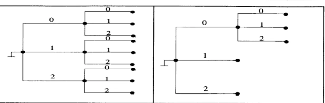
5.2. T h e c o m p l e t e D - a r y tree of length N is

t h e D - a r y tree w i t h D N leaves, each at d e p t h N from t h e root node.

Figures

2 and 3 respectively, show a c o m p l e t e 3-ary tree

and an i n c o m p l e t e 3-ary tree of length N = 2.

Definition

5.3. A code is

prefix-free

if no codeword in t h e

code is a prefix of a n o t h e r codeword in t h e same code. As an example, t h e code with codewords 0 and 011 is not prefix-free. A prefix-free code has the p r o p e r t y t h a t a codeword is recognizable as soon as its last digit is known. This ensures t h a t if a sequence of digits corresponding to several codewords in t h e code are w r i t t e n contiguously, t h e n t h e codewords from t h e sequence can be read out instantaneously. For example, suppose t h e codewords of a code are u 1 = 0, u2 = 10, u 3 = 110 and u4 = 111. T h e n the following sequence of digits 011010010 corresponds to t h e codewords Ul, u3, u2, ul, u2.

Figure 2. A complete 3..ary tree of length 2.

Figure 3. An Incomplete 3- ary tree of length 2.

A prefix-free code has the property that a codeword is recognizable as soon as its last digit is known.

(12)

62

There exists a D- ary prefix-free code whose code- lengths are the positive integers

wt,w 2 ... w Kifand only if

~ I K D -~ < 1.

For the rest of the article, we restrict our attention to prefix-free codes. Every D-ary prefix-free code can be represented on a D-ary tree wherein the set of codewords in the code correspond to a set of leaf nodes in the D-ary tree and the length of a codeword is equal to the depth of the corresponding leaf node from the root node. We now state a necessary and sufficient condition for the existence of prefix-free codes.

L e m m a 5.1 ( K r a f t ' s Inequality): There exists a D-ary prefix-free code whose code-lengths are the positive integers Wl,W2,...,Wg if and only if

K

~

D -~i < 1.

i = l

Proof. Observe that in a complete D-ary t r e e of length

N , D N - w leaves stem from each node that is at depth w from the root node, for w < N.

Suppose there exists a D-ary prefix-free code whose code- lengths are Wl, w 2 , . . . , Wg. Without loss of generality, let Wl < w2 < ... _< wK. Let N = m a x i w i = W g . We will now construct a tree for the prefix-free code starting with a complete D-ary tree of length N. Order the leaves at depth N in some fashion. Starting with i = 1 and the first leaf node zl, if Wl < N, identify the node, say v, in the tree that is at depth wl and from where the leaf node z 1 stems. Delete the portion of the tree from v down to its leaves. By this process, we make this vertex v a leaf node at depth Wl. For i = 2, identify the next leaf node z2 not equal to v. Find a node v2 at depth w2 from which z2 stems and delete the subtree from v2 down to its leaves, thereby making v2 a leaf node. Similarly, repeat the process for i = 3, 4 , . . . , K. By this process, at each step, D N-wl leaf nodes in the original complete D-ary tree are deleted. However, since the complete D-ary tree contained only D g leaf nodes, we have D N - ~ I + D N-w2 + . . . "4- D g - w K <_ D N. Dividing by D g gives the desired condition.

(13)

GENERAL I ARTICLE

To prove t h e converse, suppose w l , w 2 , . . . , W K are positive integers satisfying the inequality )--~'~=z D - ~ -< 1 (*). Then, w i t h o u t loss of generality, let wl _< w2 _< 9 .. _< wK. Set N = m a x / w i = wK. We want to show t h a t we are able to construct a prefix-free code with codeword lengths wl, w 2 , . . . ,wK. Start again with t h e .complete D-ary tree.

Let i = 1. Identify a n o d e zl at d e p t h wl to be the first codeword of t h e code we intend to construct. If Wl < N , delete the subtree s t e m m i n g from z 1 down to its leaves so t h a t Zl becomes a leaf node. Next, i n c r e m e n t i by 1 a n d look for a n o d e zi in t h e remaining tree which is not a codeword and is at d e p t h w~. If there is such a node, call this the i t h codeword and delete t h e subtree s t e m m i n g from zi down to its leaves. Repeat t h e above process by incrementing i by 1. This algorithm terminates w h e n either i > K or w h e n t h e algorithm c a n n o t find a n o d e zi satisfying t h e desired p r o p e r t y in t h e i t h step for i <_ K. If the algorithm identifies K codeword nodes, t h e n a prefix-free code can be constructed by labeling the edges of the tree as follows: At each node, label the r _< D edges t h a t s t e m from it as 0, 1, 2 . . . , r - 1 in any order. T h e ith codeword is t h e n the sequence of edge-labels from the root n o d e up to t h e i t h codeword node.

T h e only part r e m a i n i n g to be seen is t h a t the above algorithm will not t e r m i n a t e before K codeword nodes have been identified. To show this, consider the i t h step of this algorithm w h e n Zx, z 2 , . . . , zi-1 have been identified and zi needs to be chosen. T h e n u m b e r of surviving leaves at d e p t h N not s t e m m i n g from any codeword is

D N " ( D N-w1 Jr" D N-w2 + . . . + D N - W ~ - l ) . But by our assumption (.), this n u m b e r is greater t h a n zero. Thus, there exists a n o d e z~ which is not a codeword and which is at d e p t h w~ in t h e tree t h a t remains at step i. Further- more, since wi _> wi-1 _> w i - 2 . . . _> Wx, the n o d e zi will not lie in any of t h e p a t h s from the root n o d e to any of

If the algorithm identifies K codeword nodes, then a prefix- free code can be constructed by labeling the edges of the tree as follows: At each node, label the r <_ D edges that stem from it as 0,1,2 .... r-1 in any order. The i th codeword is then the sequence of edge- labels from the root node up to the i th codeword node.

(14)

GENERAL [ ARTICLE

The depth of a codeword-node is equal to the length of the codeword in the code, and the codeword is the sequence of edge- labels on this tree from the root node up to the corresponding codeword-node.

zl, z 2 . . . , zi-1. This argument holds for i = 1, 2 , . . . , K; hence, this algorithm will always be able to identify K codeword nodes and construct the corresponding prefix-

free code. 9

A. Trees with Probability A s s i g n m e n t s

Let us suppose that there is a D - a r y prefix-free code that maps symbols from a source U onto D-ary strings such that the mapping is invertible. For convenience, let ul, u 2 , . . . , u g be the source symbols and let the codewords corresponding to these symbols also be denoted by Ux, u 2 , . . . , UK. The proof of the Kraft inequality tells us how to specify a D-ary prefix-free code on a D-ary tree. T h a t is, a D-ary tree can be built with the edges labeled as in the proof of Lemma 5.1 such that the codewords are specified by certain leaf nodes on this tree, the depth of a codeword-node is equal to the length of the codeword in the code, and the codeword is the sequence of edge-labels on this tree from the root node up to the corresponding codeword-node. Furthermore, probabilities can be assigned to all the nodes in the tree as follows: assign the probability

p(ui)

for the codeword node which corresponds to the codeword ui (or, the source symbol ui.) Assign the probability zero to a leaf node that is not a codeword node. Assign a parent node (that is not a leaf node), the sum of the probabilities of its children nodes. It is easy to verify that for such an as- signment, the root node will always have a probability equal to 1. Such a D-ary tree gives a complete description of the D-ary prefix-free code. This description will be useful in describing two specific coding methods: the Shannon-Fano coding algorithm and the Huffman coding algorithm.

B. Source Coding Theorem f o r Prefix-Free Codes

Before we present the two coding techniques, we present another version of the source-coding theorem for the

(15)

GENERAL J ARTICLE special case of prefix-free codes:

Theorem

5.1. Let g~, g ~ , . . . , g* be the optimal codeword lengths for a source with distribution

p ( X )

and a D- ary alphabet, and let L* be the corresponding expected length of the optimal prefix-free code

(L -- Y]iPig).

Then

H D ( X ) < L <_ H D ( X ) + 1.*

Proof.

We first show t h a t the expected length L of any prefix-free D-ary code for a source described by the random variable X with distribution

p ( X )

is at least the entropy

H D ( X ).

To see this, let the code have codewords of length

gl,g2,..,

and let the corresponding probabilities of the codewords be

Pl,P2, ....

Consider the dif- ference between the expected length L and the source entropy

H o ( X ) ,

i L - M o ( x ) = logo

"-"i

"-'i

Pi

logo

D - l ' +

log

i i

Let

r, = D-t'/()-~j D-t~)

and c -- ~-]j D-t~. Then,

L - H o ( X ) = E p l

log O P--/- log O c.

i ri

The first term on the right-hand side is a well-known term in information theory, called the 'divergence' between the probability distributions r and p can be shown to be non-negative. (See [2]). The second term is also non-negative since c < 1 by the Kraft inequality. This shows that

L - H D ( X ) > O.

Suppose there is a prefix-free code with codeword lengths gl, g2,.., such that

gi --

[logo ~ ] . Then the

gi's

satisfy the Kraft inequality since

~-]i D-e~ < ~-]i Pi

= 1. Fur- thermore, we have 1 1 l O g D - - - - < g i < - - l O g D - - + l . Pi Pi The expected length L of any prefix-free D-ary code for a source described by the random variable X with distribution p(X) is at least the entropy

Ho(X ).

RESONANCE I February 2006

(16)

GENERAL [ ARTICLE

This theorem says that an optimal code will use at most one bit more than the source entropy to describe the source alphabets.

Hence, the expected length L of such a code satisfies

HD(X ) =

Z p i l o g D 1 < L

Pi i 1 + I ) = H o ( X ) + I .

Pi~'i <-- ~ Pi(lOgD P-7

i i

Since an optimal prefix-free code can only be better than the above code, the expected length L* of an optimal code satisfies the inequality

L < L < HD(X) +1.*

Since we have already shown that any prefix-free code must have an expected length which is at least the entropy, this proves that

HD(X) < L < HD(X ) -t-*

1.

Note that in the above theorem, we are trying to find a description of all the alphabets of the source individu- ally. This theorem says that an optimal code will use at most one bit more than the source entropy to describe the source alphabets. In order to achieve a better compression, we can find a corresponding code for a new source whose alphabets are sequences of length n > 1 of the original source X. As n gets larger, the corresponding optimal code will have an effective code-length as close to its source entropy as possible. In fact, it can be shown that the effective code-length for an optimal code then satisfies

H ( X ) <

E[~Xn] * <

H ( X ) + .~.

This result is in accordance with Theorem 4.1 of Section 4.

C. S h a n n o n - F a n o Prefix-Free Codes

Following the proof-technique of Theorem 5.1, we present a natural source-coding algorithm t h a t is popularly known as the Shannon-Fano algorithm. For a source U, this algorithm constructs D-cry prefix-free codes with expected length at most one more than the entropy of the source. The algorithm is as follows:

(17)

(i)

Suppose t h e source U is described by the source symbols ul, u 2 , . . . , Ug having probability of occur- rences Pl = P(uz),P2 = p ( u 2 ) , . . . , p K = p ( u g ) , respectively. T h e n , for i = 1, 2 , . . . , K , set wi = [log O ~ ] to be t h e length of t h e codeword corresponding to ui. Observe t h a t t h e sequence of wi's satisfies t h e K r a f t inequality since

D - ' ~ < ~ Pi = 1.

i i

(ii) Using t h e a l g o r i t h m m e n t i o n e d in t h e proof of the K r a f t - i n e q u a l i t y ( L e m m a 5.1), a D - a r y tree is grown such t h a t t h e codeword nodes are at d e p t h s wl, w 2 , . . . , W g on this tree. T h e sequence of edge labels from t h e root n o d e to a c o d e w o r d n o d e specify t h e c o d e w o r d of the S h a n n o n - F a n o code.

The effective code length of the

Shannon-Fano code is then Zip i w r This quantity is less than Ho(U)+I from the proof of Theorem 5.1.

We can f u r t h e r assign probabilities to t h e nodes of this tree as m e n t i o n e d before. T h e effective code length of the S h a n n o n - F a n o code is then ~-~iPiWi. This q u a n t i t y is less t h a n H o ( U ) § 1 from t h e proof of T h e o r e m 5.1. E x a m p l e 5.1. C o n s i d e r a source U w i t h a l p h a b e t set / / = {ul, u2, u3, u4, us} with the probability of occur- rences p ( u l ) = 0.05,p(u2) = 0.1,p(u3) = 0.2,p(u4) = 0.32,p(u~) = 0.33. For D = 2, t h e lengths of t h e codewords for a S h a n n o n - F a n o binary prefix free code are wl = [log 20.-~5] --- 5, w2 = [log 20Af] = 4, w3 =

_._1]=

~ ] = 3, w4 = [log 2 0.-~2] = 2, a n d w 5 = [log 2 0.33 [l~ 0.2

2. T h e S h a n n o n - F a n o algorithm constructs a (D = 2) binary tree as shown in Figure 4. T h e codewords cor- responding to ul, u2, u3, u4, u5 are 00000, 0001,010, 10, 11, respectively. T h e average code-length is 5 9 0.05 + 4 9 0.1 + 3 9 0.2 + 2 9 0.32 + 2 9 0.33 = 2.55 bits and t h e entropy of t h e source is 2.0665 bits.

(18)

24

0 0

t

. 3 5 0 0 ~ 0 . 1 5

l

,

i

0 . 1 5 I o 0 e 0 . 2 u 3

l

O . 2 1 o c) : 0 . 3 2 i 0 . 6 5 u 5 ! --- 0 . 3 3 U 1 0 -- o . o s 1 o ~ 0 . i u 2 Figure 4. A Shannon-Fano binary prefix.free code.

6. Huffman Coding

This section presents Huffman's algorithm for construct- ing a prefix-free code for a source U. The binary case is considered first where we obtain an optimal binary prefix-free code. The more general D-ary case, for D > 2, is considered next.

A . B i n a r y Case

The objective of Huffman coding is to construct a binary tree with probability assignments such that a chosen set of leaves in this tree are codewords.

Using the notion of trees with probabilities, the objective of Huffman coding is to construct a binary tree with probability assignments such that a chosen set of leaves in this tree are codewords. We will first show that to obtain an optimal code, the binary tree that we construct must satisfy the following two lemmas.

Lemma

6.1. The binary tree of an optimal binary prefix- free code for U has no unused leaves.

Proof.

Suppose to the contrary that there is a leaf node v in the binary tree that is not a codeword, then there

(19)

is a parent node v ~ t h a t has v as its child node. Since the tree is binary, v has another child node u. Suppose u is a codeword node corresponding to the codeword c, then deleting u and v and representing v ~ as the codeword node c yields a code with a lower average code-length since we have reduced the code-length for the codeword c without affecting the code lengths of the remaining codewords. However, since we assumed that the binary tree represented an optimal code to begin with, this is

a contradiction. 9

L e m m a 6.2. There is an optimal binary prefix-free code for U such that the two least likely codewords, say Ug_ 1

and Ug, differ only in their last digit.

Proof. Suppose we have the binary tree for an optimal code. Let ui be one of the longest codewords in the tree. By Lemma 6.1, there are no unused leaves in this tree, so there is another codeword uj which also has the same parent node as ui. Suppose uj ~ Ug, then we can interchange the codeword nodes for uj and uK. This interchange will not increase the average code-length since

p(Ug) < p(uj)

and since the code-length of Ug is at least the code-length of uj in the original code. Now if

ui ~ Ug-1, we can similarly interchange the codeword nodes for ui and uK-1. Thus, the new code has u/~ and

Ug-1 among its longest codewords and uK and Ug-1

are connected to the same parent node. Since the codewords are obtained by the sequence of edge-labels from the root node up to the corresponding codeword nodes, the codewords for u g and uK_ 1 differ only in their last

digit. 9

The above two lemmas suggest that to construct an optimal binary tree, it is useful to begin with the two least likely codewords. Assigning these two codewords as leaf nodes that are connected to a common parent node gives part of the tree for the optimal code. The parent node is now considered as a codeword having a probability that

The above two

l e m m a s suggest that to construct an

optimal binary tree, it is useful to begin with the two least

likely codewords.

(20)

Consider the problem of twenty questions where we wish to find an efficient series of yes-or-no questions to determine an object from a class of objects. Suppose the probability distribution of the objects in this class is known a priori and it is assumed that any question depends on the series of answers received before that question is to be posed, then the Huffman coding algorithm provides an optimal solution to this problem.

is t h e sum of t h e probabilities of t h e two leaf nodes a n d t h e two codewords c o r r e s p o n d i n g to t h e leaf nodes are now ignored. T h e algorithm proceeds as before by considering t h e two least likely c o d e w o r d s t h a t are available in t h e new code and constructs t h e subtree corresponding to these vertices as before.

Huffman's a l g o r i t h m for c o n s t r u c t i n g an o p t i m a l b i n a r y prefix-free code for a source U w i t h K symbols is sum- marized below. It is a s s u m e d t h a t

P(u) ~ 0

for all u E / 4 . T h a t is, no codeword will be assigned to a symbol u E / 4 t h a t has a probability of occurrence equal to zero.

(i)

Assign labels, i.e., ul, u 2 , . . . ,

UK

to K vertices which will be t h e leaves of t h e final tree, and assign the probability

P(ui)

to t h e vertex labeled ui, for i =

1 , . . . , K . Let these K vertices be called 'active' vertices.

(ii)

Create a new node v a n d join t h e two least likely active vertices ui and uj (i.e., two vertices with t h e least probabilities) to v. T h a t is connect v to ui and uj. Assign the labels 0 a n d 1 to the two edges (v, ui) a n d (v, uj) in any order.

(iii)

D e a c t i v a t e the two vertices c o n n e c t e d to v a n d ac- tivate t h e node v. Assign t h e n e w active vertex v the s u m of the p r o b a b i l i t i e s of ui and uj.

(iv)

If t h e r e is only one active vertex, t h e n call this t h e root vertex and stop. Otherwise, r e t u r n to Step

(ii).

Example

6.1. Consider a source U w i t h a l p h a b e t set /4 = {ul, u2, u3, u4, us} with t h e probability of occurrences

p(ul)

= 0.05, p(u2) = 0.1,p(u3) = 0.2,p(u4) -- 0.32,p(us) = 0.33. T h e Huffman coding algorithm constructs a b i n a r y tree as shown in

Figure

5. T h e codewords corresponding to u 1, u2, u3, u4, u5 are 000, 001,01,

(21)

GENERAL J ARTICLE 0 1 1 0

t

, 0 . 3 5 1 "L& :1_ L o ~ 0 . 0 5 - 0 . 1 5 1SL 2 1 o 0 . 1 1.1 3 e 0 . 2 0 e 0 . 3 2 0 . 6 5 1 ] - 1 5 o 0 . 3 3

Figure 5. An (opUmal) bi- nary Huffman code.

10, 11, respectively. The average code-length is 3.0.05 + 3.0.1 + 2 . 0 . 2 + 2 . 0 . 3 2 + 2 - 0 . 3 3 = 2.15 bits. Note that this number is smaller than the average code-length of the Shannon-Fano code in Example 5.1.

Example 6.2. Consider the problem of twenty questions where we wish to find an efficient series of yes-or-no questions to determine an object from a class of objects. Suppose the probability distribution of the objects in this class is known a p r i o r i and it is assumed that any question depends on the series of answers received before that question is to be posed, then the Huffman coding algorithm provides an optimal solution to this problem.

B . D - a r y c a s e

The algorithm for the binary case can be easily gener- alized to construct an optimum D-ary prefix-free code. The following two lemmas, which are the extensions of Lemmas 6.1 and 6.2 for the D-ary case, are stated without proof [3].

L e m m a 6.3. The number of unused leaves for an optimal D-ary prefix-free code for a source U with K possible values, K _> D, is the remainder when ( K - D ) ( D - 2) is divided by D - 1.

L e m m a 6.4. There is an optimal D-ary prefix-free code for a source U with K possible values such that the D - r

There is an optimal D-ary prefix-free code for a source U with K possible values such that the D - r least likely codewords differ only in their last digit, where r is the remainder when

(K-D)(D-2)

is divided by D - I .

(22)

GENERAL J ARTICLE

least likely c o d e w o r d s differ only in t h e i r last digit, w h e r e r is t h e r e m a i n d e r w h e n ( K - D ) ( D - 2) is d i v i d e d by D - 1 .

B a s e d o n t h e two l e m m a s , H u f f m a n ' s a l g o r i t h m for con- s t r u c t i n g an o p t i m a l D - a r y prefix-free code (D > 3) for a source U w i t h K symbols, s u c h t h a t P ( u ) # 0 for all u, is given by:

Figure 6. An (optimal) 3-ary Huffman code.

(i)

(ii)

(iii)

(i,)

Label K vertices as u l , u 2 , . . . , u K a n d assign t h e p r o b a b i l i t y P ( u i ) to t h e v e r t e x l a b e l e d ui, for i -- 1, 2 , . . . , K . Call t h e s e K vertices 'active'. Let r be t h e r e m a i n d e r w h e n ( g - D ) ( D - 2) is d i v i d e d b y D - 1.

F o r m a n e w n o d e v a n d c o n n e c t t h e D - r least likely active vertices to v via D - r edges. Label t h e s e edges as 0, 1, 2 , . . . , D - r - 1 in a n y r a n d o m order.

D e a c t i v a t e t h e D - r active vertices t h a t are con- n e c t e d to t h e n e w n o d e v a n d a c t i v a t e v. Assign v t h e s u m of t h e p r o b a b i l i t i e s of t h e D - r deacti- v a t e d vertices.

If t h e r e is only one active v e r t e x r e m a i n i n g , t h e n call this v e r t e x t h e r o o t n o d e a n d stop. O t h e r w i s e , r e t u r n t o S t e p (ii). / 0 U 2_ 8 0 . 0 5 t 1 U 2 0 . 3 5 8 . 0 . 1 2 U 3 Q 0 . 2 -:- 0 . 3 2 U 4 U 5 -r. 0 . 3 3 72 _{RESONANCE J February 2006}

(23)

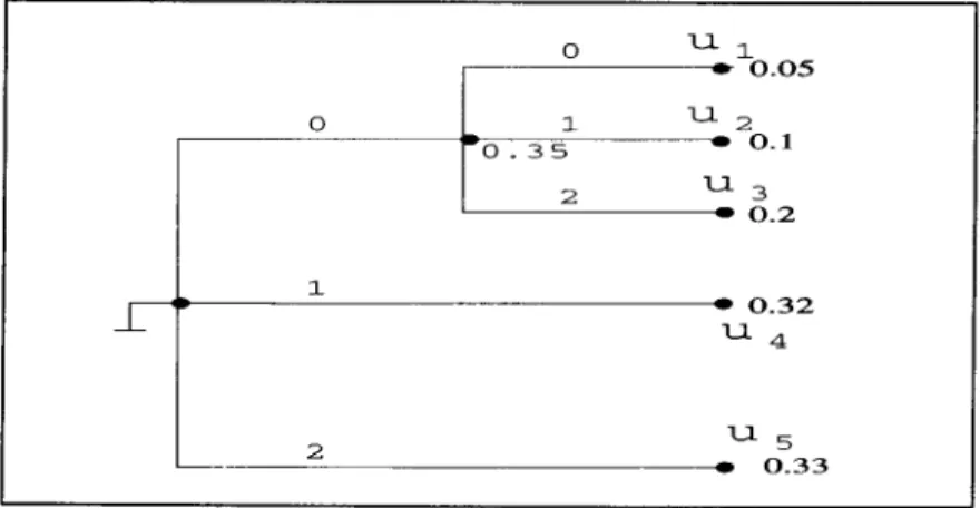
Example

6.3. Consider the same source U as in Example

6.1. The Huffman coding algorithm constructs a 3-ary prefix-free code as shown in

Figure

6. The codewords corresponding to ul, u2, u3, u4, u5 are 00, 01,02, 1, 2, respectively. The average code-length is 2-0.05 § 2 . 0 . 1 § 2 9 0.2 + 1 9 0.32 + 1 9 0.33 = 1.35 ternary digits and the entropy of the source is H3(U ) = 1.3038 ternary digits.

Remark

6.1. While the proof of Theorem 5.1 seems to

suggest that the Shannon-Fano coding technique is a very natural technique to construct a prefix-free code, it turns out t h a t this technique is not optimal. To illustrate the sub-optimality of this technique, consider a source with two symbols ul and u2 with probability of occurrences p(ul) = 1/16 and p(u2) = 15/16. The Shannon-Fano algorithm finds a binary prefix-free code with codeword lengths equal to Flog 2 T~16] = 4 and Flog 215--~T61~] = 1, respectively, whereas the Huffman- coding algorithm yields a binary prefix-free code with codeword lengths equal to 1 for both.

7. S u m m a r y

This article has presented a derivation of the best achievable performance for a source encoder in terms of the average code length. The source-coding theorem for the case of prefix-free codes shows that the best coding scheme for a source X has an expected code-length bounded between

H(X)

and

H(X)

+ 1. Two coding techniques, the Shannon-Fano technique and the Huff- man technique, yield prefix-free codes which have expected code-lengths at most one more than the source entropy. The Huffman coding technique yields an optimal prefix-free code yielding a lower expected code- length compared to a corresponding Shannon-Fano code. However, the complete proof of the optimality of Huff- man coding [2] is not presented here; Lemma 6.1 only presents a necessary condition that an optimal code must satisfy.

aditt.pdf

[4] R L Karandiksr,OnRan- domness and Probability: How to Model Uncertain Events Mathematically,

Resonance, VoL 1, No.2, Feb. 1996.

[5] WFeller, Anlmroductionto

Pvobab~ ~ o ~ and ~s

Applications, Vols.1,2, Wiley-Eastern, 1991. [6] S Natarajan, Entropy, Cod-

ing and Data Compression,

Resonance, VoL6, No.9, 2001.

Address for Correspondence Deepak Sridhara Inslilul for Mathematik

Universit~t ZOrich Emaih sridhara@malh.unizh.ch