Why
are grammatical elements more evenly dispersed than
lexical
elements? Assessing the roles of text frequency and
semantic
generality
Martin Hilpert
1and David Correia Saavedra
1Abstract
Grammatical elements such as determiners, conjunctions or pronouns are very evenly dispersed across natural language data. By contrast, the uses of lexical elements have a stronger tendency to occur in bursts that are interspersed by long lulls. This paper considers two alternative explanations for this difference. First, it could be hypothesised that the more even distribution of grammatical elements is merely an effect of an element’s high text frequency. Alternatively, it could be argued that a more even distribution is a symptom of greater generality in meaning. In order to assess the impact of both frequency and semantic generality, we conducted a corpus-based study that contrasts lexical and grammatical elements in Present-Day English. Our results suggest that evenness of dispersion is chiefly an effect of high frequency.
Keywords: abstractness, deviation of proportions, dispersion, distributional semantics, grammaticalisation.
1. Introduction
Highly grammaticalised elements, such as determiners (the, an), conjunctions (and, because) or pronouns (she, yours), are not only very frequent in running text, but they also tend to be very evenly dispersed. A randomly chosen sentence from a book written in English is very likely to contain the determiner the, and crucially, so are the following sentences. By contrast, lexical items, or content words, do not attain the same level of text frequency, and they usually show a distribution that is characterised by bursts 1Université de Neuchâtel, Institut de langue et littérature anglaises, Espace Louis-Agassiz 1, CH-2000 Neuchâtel, Switzerland.
rabbit (n=48)
running words
0 5000 10000 15000 20000 25000
Figure 1: The distribution of the word rabbit in Alice’s Adventures in Wonderland.
and lulls. To illustrate, the word rabbit is quite frequent in Lewis Carroll’s Alice’s Adventures in Wonderland. There are forty-eight instances in about 27,000 words. However, the reader is not likely to come across one instance of rabbit on every other page. Rather, as is shown in Figure 1, the uses of rabbit are densely clustered in relatively few passages.
This contrast between lexical and grammatical elements gives rise to the main question of this paper: why are grammatical elements more evenly dispersed than lexical elements? Two alternative answers suggest themselves. First, it could be hypothesised that the more even dispersion of grammatical elements is to be fully explained as a (trivial) effect of high text frequency: the more tokens of a given type we find in a corpus, the higher the likelihood that a given chunk of that corpus will contain at least one token. In this view, more frequent elements should be more evenly dispersed, regardless of whether the respective elements would be seen as clearly grammatical (the, on or because), clearly lexical (rabbit, sweet or arrange), or somewhere in the middle of the continuum between lexical and grammatical (start or help in ‘start packing’ or ‘help to explain’). Elements with identical frequencies should be dispersed in similar ways. To give an illustration, in the British National Corpus (BNC), the lexical noun time and the preposition about are equally frequent, hence the evenness of their respective dispersions should be similar. In the following, we will refer to this view as the frequency hypothesis. As an alternative to this hypothesis, it could be argued that a more even dispersion is a symptom of the more abstract, schematic word meaning that is conveyed by grammatical elements. We will call this view the semantic generality hypothesis. The hypothesis can be illustrated with a lexical noun such as rabbit, which conveys a meaning that is very concrete. By contrast, a complex preposition, such as by means of, captures a highly abstract idea. Both elements occur with approximately the same frequency in the BNC, so that according to the frequency hypothesis, their dispersion should be roughly identical. According to the semantic generality hypothesis, however, the complex preposition should be distributed more evenly than the noun.
The two hypotheses have implications not only for the patterning of linguistic elements in synchronic corpus data but also for language change. Taking our cues from research into grammaticalisation (Hopper and Traugott, 2003), we do not assume a categorical distinction between lexical and grammatical elements. Rather, we subscribe to the view that the difference between the two is gradual, and that grammatical elements can develop out of lexical words and constructions. Importantly, it is not in contradiction to this view to distinguish between elements that are grammatical (shall, because, that, etc.) and elements that are lexical (rabbit, write, yellow, etc.). Some linguistic forms are clearly grammatical and are thus situated at one end of the grammar–lexicon continuum, whilst others are clearly lexical, so that they are found at the other end of the continuum. By selecting elements from both groups and investigating contrasts between them, we can determine what typically characterises elements at either end of the continuum.
Our study is organised in the following way. Section 2 reviews corpus-linguistic work on dispersion and related notions, thereby providing a theoretical background for our analysis. Section 3 sets out to test the frequency hypothesis and the semantic generality hypothesis on the basis of synchronic data from the British National Corpus. Using a database of seventy lexical elements and seventy grammatical elements, we measure the dispersion of all elements and present the results of a regression analysis that tries to model dispersion in terms of frequency and semantic generality. Our conclusions are presented in Section 4. To preview our main finding, our results suggest that evenness of dispersion is first and foremost an effect of high frequency. The analysis of data from the BNC indicates that semantic generality, as measured through four different qualitative and quantitative operationalisations, has a measurable effect, but this effect is not as strong and robust as the frequency effect that we observe.
2. Why should dispersion be studied, and how can we measure it? Commenting on the notion of dispersion, Gries (2010: 197) notes that ‘despite the relevance of dispersion for virtually all corpus-linguistic work, it is still a very much under-researched topic’. Dispersion is particularly relevant for research that uses text frequencies as a proxy for psychological phenomena. For example, text frequency is commonly taken to reflect the cognitive entrenchment of linguistic elements. By now, a substantial body of psycholinguistic literature documents the effects that text frequency has on language processing (Ellis, 2002). Importantly, if it is not taken into account how text frequencies fluctuate locally between different parts of a corpus, it may be misleading to attribute certain psychological effects to text frequency. There is empirical evidence that the dispersion of a linguistic element may modulate known frequency effects. For instance, Adelman et al. (2006) challenge the classic finding that frequent
Category Examples
1. entities Africa, Bible, Darwin
2. predicates and relations blue, die, in
3. modifiers and operators believe, everyone, forty 4. higher-level operators hence, let, supposedly, the
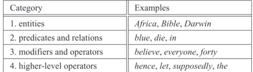
Table 1: Four semantic categories (Altmann et al., 2009: 4).
words are processed and named faster than infrequent ones (Forster and Chambers, 1973). They present the results of word naming and lexical decision tasks, arguing that the dispersion of a word predicts the observed latencies more accurately than word frequency. Gries (2008: 428) makes the point that dispersion measurements can be used to adjust observed text frequencies, so that essentially dispersion is added as a covariate to analyses that investigate a relation between frequency and some cognitive response.
In this paper, dispersion constitutes the dependent variable (i.e., the thing that is to be explained in terms of other factors). Previous research that has addressed our research question includes work by Altmann et al. (2009), who model the so-called ‘burstiness’ of words, which is the distribution of word recurrence time – the time intervals between one use of a word and the next use. This notion is not quite identical to dispersion as such, but it is very close. Altmann et al. (2009) note that words from the same frequency range may differ substantially in burstiness, so that words like once, certainly or yet are less bursty than design, selection or intelligent (Altmann et al., 2009: 4). Meaning, or more precisely semantic generality, suggests itself as an explanation for differences of this kind. Altmann et al. (2009) operationalise semantic generality with a distinction of four meaning-based categories, which are shown in Table 1.
The categories in Table 1 are based on truth-conditional characteristics of the respective elements, which correspond to differences in how these elements can be modelled in formal semantic frameworks (see Partee, 1992). Burstiness is hypothesised to decline from Category 1 to the remaining categories. As can be seen, the categorisation cuts across the distinction of lexical and grammatical elements: blue and in share the same category, as do let and the. Altmann et al. (2009: 5) analyse web-based discussion data, finding reliable differences in the predicted order between the four semantic categories. Importantly, their results indicate that the effect of meaning disappears above a certain frequency threshold. With items that are as frequent as since or new, all categories converge on the same level of burstiness, despite differences in meaning. Pierrehumbert (2012) follows up on this work. She investigates the burstiness of deverbal nouns and their morphological sources in word pairs such as discuss and discussion. In a direct comparison of simplex verbs and derived nouns, the
nouns tend to be burstier than their sources. The explanation that is offered for this observation is that deverbal suffixes send a stem to a lower semantic category (see Table 1). Relatively more specific meanings are associated with deverbal nouns. For instance, in the pair of evolve and evolution, it is only the noun that has acquired the more specific sense of a scientific theory (Pierrehumbert, 2012: 113). Summing up this line of work, there is evidence that meaning impacts the dispersion of a linguistic element and that meaningful comparisons can be established between elements that differ in semantic generality.
Up to now, we have discussed dispersion in a non-technical way. Before we proceed to the empirical sections of this paper, we need to spell out how we will measure dispersion in corpus data. Gries (2008: 407–10) presents an overview of measures of dispersion and ends the overview by proposing yet another alternative, which he calls deviation of proportions (DP) and which we will use in our analysis. Gries outlines a number of advantages of that measure. Unlike some other measures of dispersion, DP can accommodate corpora that are divided into parts with different sizes. It further does not include a measure of statistical significance, thereby avoiding problems that might arise through the violation of assumptions. Lastly, it is conceptually straight-forward and easy to implement. The calculation of DP for a linguistic element in a corpus involves the following steps (see Gries, 2008: 415):
• A corpus is divided into parts. For each part, it is determined how much of the corpus it contains (For example, a first corpus part that holds 5,000 words and belongs to a 100,000 word corpus holds 5 percent of all the data. A second corpus part with 7,000 words would hold 7 percent, etc.).
• A linguistic element is chosen, its frequencies in the whole corpus and in all corpus parts are determined. (To illustrate, let us say that the word car appears 100 times in total, out of that total, three instances are registered in the first part.)
• For all corpus parts, absolute differences between observed and expected percentages are summed up. (Since the first corpus part contains 5 percent of the entire corpus, we expect it to contain five percent of all 100 instances of car, that is to say, five tokens. Since we only find three instances, there is a discrepancy between 5 percent that are expected and 3 percent that are observed. Differences of this kind are added up for all corpus parts.)
• The sum of all differences is divided by two.
Calculated in this way, DP yields values between 0 and 1, where 0 indicates a perfectly even dispersion and 1 indicates a maximally uneven dispersion. We will come back to the calculation of DP in Section 3.2. We close the discussion here with the remark that the values of DP will vary to some extent with the size of the corpus parts that are chosen by the researcher. It may
thus be problematic to compare DP values across corpora that are divided into parts with different sizes (Gries, 2008: 426). With these preliminaries in mind, we can now turn to empirical matters.
3. Contrasting the dispersion of lexical and grammatical elements This section analyses how lexical and grammatical items are dispersed in synchronic corpus data. The analysis aims to establish how differences in the respective dispersion patterns relate to the factors of text frequency and semantic generality. Section 3.1 offers an overview of our database. In Section 3.2, we describe how we measured dispersion for the items in the database. Section 3.3 turns to different ways of measuring the semantic generality of these items. Section 3.4 presents the results of a regression analysis that assesses the respective impacts of frequency and semantic generality. The main result of that analysis is that in the BNC, high text frequency is an excellent predictor of even dispersion. The effect of semantic generality is measurable in some of the operationalisations that we present, but, in comparison to frequency, its impact is much weaker.
3.1 Data2
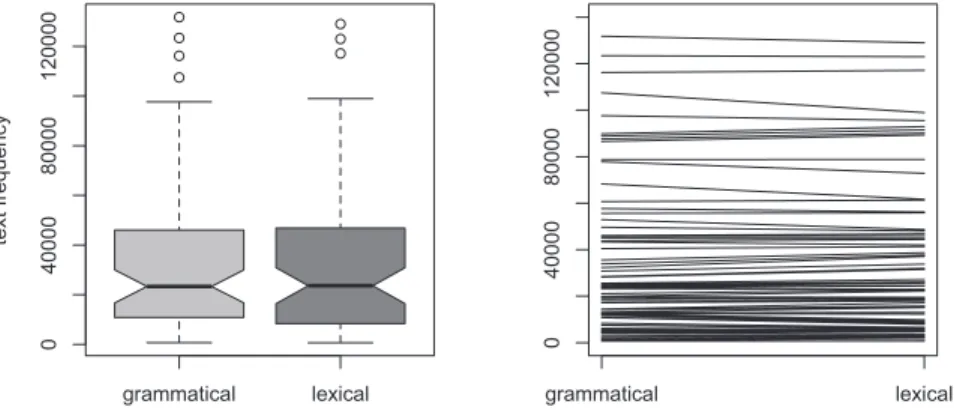
The analyses in this section are based on a database of seventy grammatical and seventy lexical elements that have been matched for text frequency in the BNC in order to ensure comparability. The matching procedure led to the exclusion of highly frequent grammatical forms such as the conjunction and or the pronoun it. There simply are no lexical elements that would be used often enough to match the frequencies of these elements. Practically, then, the analysis started with a selection of highly frequent nouns, verbs, adjectives and adverbs in the BNC. Grammatical elements from the same frequency range were selected to match those lexical forms. Elements of lesser frequency were also included, so that the complete database covers a broad frequency spectrum, ranging from approximately 1,300 instances per million words (over and just) to seven instances per million words (oneself and admittedly). The grammatical categories in the database include determiners, pronouns, prepositions, conjunctions and quantifiers. Table 2 shows a snippet of the database with the most frequent and the least frequent elements, and the full list of forms is shown in Appendix A. Words in the same row are frequency-matched.
As the number of grammatical elements in a given frequency range is limited, the text frequencies of the matched elements are not completely identical in each case. Figure 2 visualises the frequency matching with a 2For all analyses that are presented in this paper, the original data and R code for analysis are available on request.
Element BNC freq. Element BNC freq. over 131,765 just 128,996 any 123,418 know 123,000 after 116,206 see 118,253 … … … … oneself 715 admittedly 702
Table 2: Frequency-matched grammatical and lexical elements.
grammatical lexical 0 4 0000 80000 1 20000 text fr equency grammatical lexical 04 00 00 8000 01 2 0 00 0
Figure 2: Frequencies of grammatical and lexical elements in the BNC.
pair of boxplots (in the left panel) and a spaghetti plot (in the right panel). A Wilcoxon test for paired samples finds no significant difference between the two sets of frequencies (V= 1049.5, p = 0.26, 95 percent CI: –699, 275). The grammatical and lexical elements are, thus, reliably matched for text frequency, which is crucial for the subsequent analysis.
A close inspection of our list of items will reveal that the dichotomy of ‘grammatical’ and ‘lexical’ is not perfect. For instance, the element know will appear in contexts where it is clearly a lexical verb (‘I know the answer’), but also in contexts where it is part of a discourse marker (‘It was, you know, not easy’), and hence more grammaticalised. Unfortunately, this problem is hard to circumnavigate, especially for more frequent elements that tend to be polysemous. What we maintain is that the elements in our ‘grammatical’ column have a relatively greater likelihood of being used with grammatical functions than the elements in our ‘lexical’ column.
3.2 Determining the deviation of proportions for all database items The most important aspect of our analysis concerns the dispersion of our database elements across corpus data. For all elements, we measured the
deviation of proportions (Gries, 2008) in the way that is illustrated below with the element know:
• First, we divided the full BNC into 1,000-word chunks. Given that the BNC contains 100 million words, this yields 100,000 chunks. • Second, we determined the observed text frequency for each
element. In the case of know, that frequency is 123,000.
• Third, we calculated the expected frequency of know in each of our chunks. If know were completely evenly dispersed, it should appear approximately once in each of the chunks: there are 123,000 examples, so that at least one could appear in each of the 100,000 chunks. The expected percentage of know is 0.123 percent.
• Fourth, we measured the observed frequency of know in each chunk. If there is exactly one instance of know in a given chunk, this yields an observed percentage of 0.1 percent, which is just slightly lower than expected. If there are two, this yields an observed percentage of 0.2 percent, which is a bit higher than the expected percentage.
• Fifth, we took for each chunk the absolute difference between the expected percentage and the observed percentage, we added up those values, and divided the result by two. This procedure yields values between 0 and 1, where 1 indicates a maximally uneven distribution. For know, the observed value is 0.619.
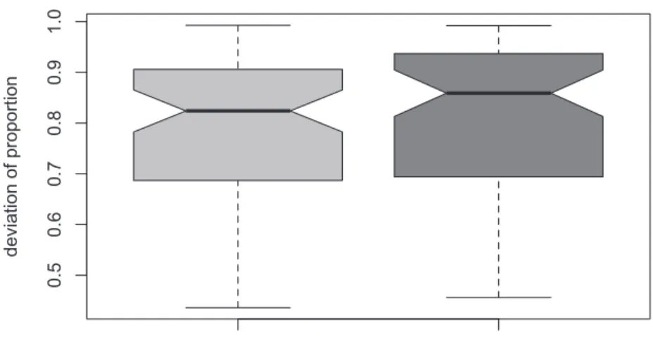
The resulting values of all elements in the database are shown in Appendix A. Figure 3 offers a visual summary by contrasting the measurements of deviation of proportions for the grammatical and lexical elements in the database. As can be seen, lexical elements have, on average, somewhat higher values (mean= 0.82) than grammatical elements (mean= 0.79). However, a Wilcoxon test for paired samples determines that deviation of proportion is not significantly greater for lexical elements (V= 1383.5, p = 0.41, 95 percent CI: –0.03, 0.08). This is already a first piece of evidence that detracts from the semantic generality hypothesis.
3.3 Determining semantic generality for all database items
In order to capture the semantic generality of the items in our database, we decided to go beyond a discrete categorical distinction such as the one taken by Altmann et al. (2009). Specifically, we decided to try out how a quantitative, distributional approach would allow us to pursue our research question. In distributional approaches to semantics, word meaning is operationalised in terms of collocational behaviour. To illustrate this idea, a lexical word such as breakfast arguably conveys a fairly concrete meaning. This characteristic is reflected by the fact that breakfast is strongly associated
grammatical elements lexical elements 0.5 0 .6 0 .7 0. 8 0 .9 1.0 d eviation of proporti on
Figure 3: Deviation of proportions of grammatical and lexical elements in the BNC.
with a specific range of other content words, such as eat, coffee, tea, morning, and so on. In a word association task, subjects would be likely to converge on these (and other) elements, so that many subjects would offer, for example, tea as an association. We call this a ‘crisp’ collocational profile. By contrast, a grammatical word such as then has a collocational profile that is much more diffuse. In a corpus such as the BNC, then is less strongly related to its respective top collocates than breakfast. This tendency can be quantified, for example by applying a measure such as pointwise mutual information. Likewise, subjects in a word association task are likely to offer a much wider and more haphazard range of associations for then than for breakfast.
One approach that uses collocational profiles for the quantification of word meaning is represented by so-called vector space models (VSMs). Applications of VSMs to linguistic research questions, notably from a variationist perspective, have been developed by Heylen and Ruette (2013) and Ruette et al. (2013). In our analysis, we follow Turney and Pantel’s (2010) practical guidelines for the creation of a semantic vector space that captures meaning similarities between words on the basis of their respective collocates. Semantic vector spaces of this kind can detect mutual similarities between the collocational profiles of all items in our database. For instance, the near-synonymous lexical items awful and bad, which are both included in the database, have fairly similar collocational profiles. By contrast, the collocational profiles of the semantically unrelated elements serious and affect differ more substantially from one another. The difference between two collocational profiles can be quantified by taking a mathematical distance measure such as the Euclidian distance or the cosine.
The idea that semantic vector spaces can capture similarities in word meaning is probably well-established enough to be uncontroversial, but
how can a semantic vector space be used to assess the semantic generality of an item? Sagi et al. (2011) used a variant of semantic vector space modelling to carry out a diachronic study of semantic broadening and semantic narrowing, thereby providing a proof of concept that gives credence to this idea. Specifically, Sagi et al. (2011) used Latent Semantic Analysis (Landauer et al., 1998) to investigate meaning change in the Old English words docga (‘mastiff dog’) and deor (‘animal’). The former of these two has undergone semantic broadening. What used to be a label for a specific breed became over time the label for an entire species. The second word underwent semantic narrowing. In Present Day English, a deer is a specific kind of animal. Sagi et al. (2011) retrieve uses of the two words from different periods of the Helsinki corpus and create context vectors for each usage event (i.e., each token of usage). Over time, the context vectors of docga and its spelling variants become more diverse, which reflects an increasingly general meaning of the word (Sagi et al., 2011: 176). Importantly, the context vectors of deor do not diversify in the same way. These results suggest that processes such as semantic broadening and narrowing, and by extension the semantic generality of a linguistic item, are in fact reflected in semantic vector spaces.
While our study is indebted to Sagi et al. (2011), our approach is different in several respects. First, while Sagi et al. create context vectors for individual tokens of usage, we are interested in types. In order to create our context vectors, we aggregate data over many usage events. Second, we do not use a ready-made implementation of semantic vector space modelling such as Latent Semantic Analysis (Landauer et al., 1998), but we developed our own algorithm that we discuss in detail below. Lastly, Sagi et al. assess semantic generality on the basis of two-dimensional scatterplots that visualise multi-dimensional scaling solutions of their context vectors. Instead of applying dimension-reduction techniques to our data, we assess semantic generality on the basis of all values in our collocate vectors. To illustrate this aspect of our approach, we reasoned that the semantic generality of words such as serious and although could be compared by measuring the relative evenness of their collocate vectors. A semantically specific word will have a crisp collocational profile in which many collocates are substantially more (or less) frequent than would be expected by chance. A semantically general word, by contrast, will have a more diffuse collocational profile in which most collocates appear just about as often as would be expected. Table 3 illustrates this with a simplified example.3
If we use the BNC to construct a collocate vector for the words house and who, and if we limit that collocate vector to the seven elements shown in Table 3, it turns out that neither of the collocates has a particular 3The seven collocates in Table 3 were chosen because they occur with who at roughly the same frequency. It goes without saying that all collocates of house and who would have to be included in order to make a meaningful comparison. The data in Table 3 are, hence, a simplified example that only serves to explain the principle of such comparisons.
house who benefit 7 (1.5) 71 (15.5) buy 84 (18.5) 61 (13.4) concerned 7 (1.5) 65 (14.2) council 138 (30.4) 67 (14.7) door 160 (35.3) 63 (13.8) goes 30 (6.6) 65 (14.2) sat 28 (6.2) 66 (14.5) TOTAL 454 (100) 458 (100) std. dev. 14.0 0.7
Table 3: (Simplified) collocate profiles of house and who. (Figures in brackets are percent.)
preference for who: all of them occur with roughly the same frequency. By contrast, the frequency profile of house shows marked preferences (buy, council, door) and dispreferences (benefit, concerned). The relative evenness of the percentages in Table 3 can be assessed by measuring the standard deviation. For house, we obtain a much higher value than for who. We will come back to this idea below, but first we briefly describe how we constructed our semantic vector space model:
• For each word in the database, we retrieved a concordance from the BNC with four words to the left and four words to the right. • From those concordances, we removed punctuation and highly
common words, using a list of 150 stopwords.4 This is a common procedure that helps to reduce noise in the statistical analysis. • We also removed all collocates that occurred less often than 1,000
times in the set of all concordances, which combine to form a corpus of about 28 million words. This was done to keep the computational effort manageable.
• We then arranged all cleaned concordances in a table in which the database elements were the column labels (140) and their collocates were in the rows (2,310). The cells of that table were filled with the observed co-occurrence frequencies of all database items with all collocates. For instance, our database contains the element above, which co-occurs six times with the collocate active in the BNC when a text window of 4L and 4R is used.
• We took those raw co-occurrence frequencies in the table and weighted them by applying pointwise mutual information (PMI). 4The list of stop words is included in our R code, which is available on request.
This is done to control for the differences in text frequency between the database items. Our subsequent analysis is based on the resulting PMI values, which thus replace the raw frequency values. This procedure left us with a table that has our 140 database items as its columns, and 2,310 rows for the collocates that allow us to distinguish between the database items. A brief illustration of these results is in order. For the adjective private, the collocates with the highest PMI values are sector and rooms. The top collocates of the adjective serious are injury and consequences. This shows that the semantic inter-relations of lexical elements are indeed captured by our semantic vector space. Grammatical elements yield somewhat less clear-cut results: the top collocates of the pronoun itself are finds and sufficient; for the negative element nor, the items with the highest PMI values are necessarily and indeed. These results warrant the interpretation that the semantic vector space model has approximately the same difficulties that a human subject would have in a word association task. If the collocational profile of a word is very diffuse, the associations are less predictable.
Any test of the semantic generality hypothesis will only be as good as the operationalisation of meaning that is applied: if a given measure of semantic generality fails to correlate with even dispersion, this constitutes evidence against the semantic generality hypothesis only so far as the measure really aligns with native speaker intuitions about word meaning. In other words, the semantic generality hypothesis is relatively vulnerable to spurious criticism, so that we have to weigh the evidence carefully. In order to treat the semantic generality hypothesis as fairly as possible, we adopted four different measures that are designed to capture different aspects of meaning, which we describe below.
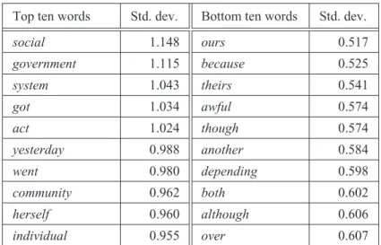
For our first operationalisation of semantic generality, we took the vectors of PMI values for all elements in our database and determined the standard deviation for each vector. Table 4 shows, in the left column, the ten elements with the highest standard deviation values, which we expected to have highly specific lexical meaning. To the right, the table displays the ten elements with the lowest standard deviation values. The latter have relatively diffuse collocational profiles and would hence be assumed to carry highly abstract or general meaning.
The left-hand elements in Table 4 do indeed convey fairly specific concepts (e.g., social, government); the lower half of Table 4 contains a number of highly abstract grammatical elements (e.g., although, theirs and because). The ten elements with the largest standard deviation values contain one element that is grammatical (herself ), and the ten elements with the smallest standard deviation values contain only one lexical element (awful). Since our database does not contain many highly concrete items such as dog or chair, nor any high-frequency grammatical elements such as the or of, it is not too surprising that the differentiation of lexical and grammatical elements in Table 4 is not completely discrete.
Top ten words Std. dev. Bottom ten words Std. dev. social 1.148 ours 0.517 government 1.115 because 0.525 system 1.043 theirs 0.541 got 1.034 awful 0.574 act 1.024 though 0.574 yesterday 0.988 another 0.584 went 0.980 depending 0.598 community 0.962 both 0.602 herself 0.960 although 0.606 individual 0.955 over 0.607
Table 4: Elements whose collocate vectors exhibit the largest and the smallest standard deviation values.
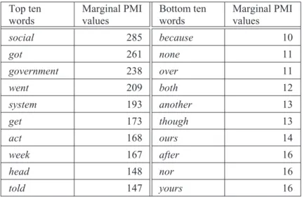
The second operationalisation of semantic generality that we employed also made use of the PMI values from our semantic vector space.5 Instead of taking the standard deviation of these values, our second measure is a simple count of values that fall outside the range of –2 to +2. These (arbitrarily chosen) cut-off points exclude the central 97 percent of all PMI values, leaving us with the 1.5 percent most positive values and the 1.5 percent most negative values. The rationale behind counting marginal PMI values is the idea that semantically specific words – that is, those with a ‘crisp’ collocational profile – will have a relatively high ratio of collocates to which they are strongly attracted and which thus have high PMI values (e.g., private and its collocates sector and rooms). By the same token, the semantic specificity of words will also prohibit certain lexical combinations and thus bring about a large ratio of collocates with very low PMI values. To illustrate this idea, the semantically specific element private has PMI values below two for thirty-eight collocates and PMI values above two for twenty-four collocates, that is, sixty-two marginal values in total. By contrast, the grammatical element though has only twelve collocates with PMI values below two and one collocate with a PMI value above two, yielding thirteen collocates with marginal values. Table 5 shows that this measure accurately discriminates between lexical and grammatical elements. All of the top ten words are lexical, whereas all of the bottom ten words are grammatical.
The third operationalisation of word meaning that we include in our analysis is the four-fold qualitative distinction used by Altmann et al. (2009). We classified the items in our database into the four categories of entities 5We would like to thank an anonymous reviewer for suggesting a variant of this procedure to us.
Top ten words Marginal PMI values Bottom ten words Marginal PMI values social 285 because 10 got 261 none 11 government 238 over 11 went 209 both 12 system 193 another 13 get 173 though 13 act 168 ours 14 week 167 after 16 head 148 nor 16 told 147 yours 16
Table 5: Elements whose collocate vectors exhibit the most and the fewest PMI values smaller than –2 and larger than +2.
(England and Australia), predicates and relations (went, awful and above), modifiers (always, enough and herself ), and higher-level operators (because, such and than).
For our fourth measure of word meaning, we accessed a database of words that were rated for concreteness ratings by speakers of English (Brysbaert et al., 2014). From our 140 database items, 131 are represented in that database. The ratings for those items correlate positively with the values that we obtained on the basis of the semantic vector space (r= 0.337, p< 0.01). Importantly, the contrast between concreteness and abstractness (measured by Brysbaert et al., 2014) is not the same as the contrast between specific and general meanings. For instance, the word plant is concrete (we can think of and picture a plant) but at the same time fairly general (it includes flowers, trees, algae, moss, vegetables, etc.). Conversely, gravity is an abstract idea that is nonetheless very specific.
To sum up this section, the discussion has outlined four different measures that are designed to capture aspects of word meaning. The first two measures are quantitative operationalisations that are based on PMI values from a semantic vector space, the two other measures are based on speaker intuitions. The following section will discuss how well these measures allow us to predict how evenly a word is dispersed through a corpus.
3.4 How do frequency and semantic generality relate to dispersion? In this section, we use polynomial regression analysis in order to model dispersion as a function of two explanatory factors: text frequency and
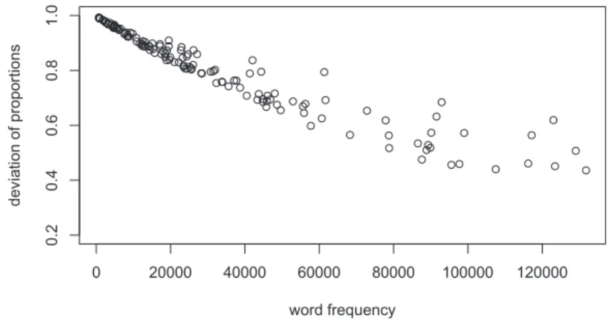
0 20000 40000 60000 80000 100000 120000 0.2 0 .4 0.6 0.8 1. 0 word frequency deviat ion of propor tions
Figure 4: Word frequency relative to deviation of proportions.
semantic generality. Dispersion is operationalised for all elements in terms of their deviation of proportions (see Section 3.2), semantic generality is captured by the four measures of word meaning that were discussed in Section 3.3. In the introduction to this paper, we identified two hypotheses that would explain dispersion as an effect of either one or the other. A more realistic assessment is that both could in fact have a role to play. In order to investigate this possibility, and in order to assess the relative impact of either factor, we used regression analysis. Figures 4 and 5 offer a first look at the data. Figure 4 shows for all elements in our database the relationship between word frequency6and deviation of proportions. The lower an element is situated on the y-axis, the more even is its dispersion.
As Figure 4 shows, increasing word frequency maps onto a curvilinear decrease of deviation of proportions. This is consonant with the frequency hypothesis: low-frequency items such as rabbit are less evenly distributed than high-frequency items such as because. Yet, it is also apparent that high-frequency items can vary considerably in their deviation of proportions. In the higher frequency ranges, towards the right side of the graph, the elements of our database are less predictable than in the lower frequency ranges.
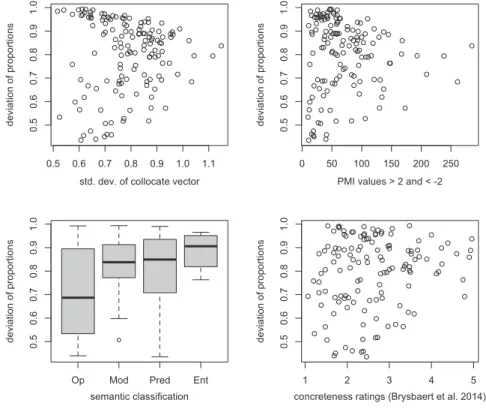
Figure 5 shows how our four meaning-related measures map onto deviation of proportions. In all four panels of Figure 5, deviation of proportions is shown on the y-axis, while the x-axis shows semantic generality or abstractness, going from the most general and abstract elements on the left towards increasingly more specific and concrete elements on the right. In all four measures, elements on the left side of the graph (i.e., semantically general or abstract elements) show a very wide range of values 6Psycholinguistic work often draws on logged frequencies rather than raw frequencies (see Baayen 2008: 33). Since both yield very similar results in our analysis, we use and report raw frequencies here for the sake of transparency and simplicity.
0.5 0.6 0.7 0.8 0.9 1.0 1.1 0.5 0 .6 0.7 0 .8 0.9 1 .0
std. dev. of collocate vector
d e vi at io n o f p ro po rt io n s 0 50 100 150 200 250 0 .5 0 .6 0 .7 0 .80 .9 1. 0
PMI values > 2 and < -2
d e vi at ion of p ro po rt io ns
Op Mod Pred Ent
0.5 0 .6 0.7 0 .8 0.9 1 .0 semantic classification devi ati on o f p rop or tions 1 2 3 4 5 0 .5 0 .6 0 .7 0. 8 0 .91 .0
concreteness ratings (Brysbaert et al. 2014)
devi ati o no f p rop o rt ion s
Figure 5: Meaning-related measures relative to deviation of proportions.
for deviation of proportions. It thus appears that general meaning does not automatically guarantee even dispersion. The four measures also indicate that elements with highly specific or concrete meanings are never evenly dispersed: the lower right corner of all four panels stays blank.
We used regression modelling to assess how well both frequency and semantic generality allow us to predict the values of our dependent variable (deviation of proportions). Since the measurements of our dependent variable are limited to the range between 0 and 1, and a regression might predict values outside that range, we transformed the values of the dependent variable using the logit function. In order to better capture the non-linear relation between word frequency and dispersion that is shown in Figure 4, we used polynomial regression. This type of regression adds for a non-linear factor a new predictor that squares the values of the original predictor (Dalgaard, 2008: 196). The remaining predictors were not transformed (i.e., they were used in the way they are shown in Figure 5). As the graphs in Figure 5 suggest, our meaning-related factors are strongly correlated with each other, which means that including all of them in a single regression model would lead to multi-collinearity and is thus not advisable (see Baayen, 2008: 40). We have therefore constructed four separate models that combine
Estimate Std. error t p
Intercept 3.356 0.07 47.05 <0.001 ***
Word freq. –8.12E–05 3.59E–06 –22.62 <0.001 ***
Word freq. (squared) 4.59E-10 3.10E-11 14.67 <0.001 ***
PMI values <–2 and >+2 2.35E-03 1.49 3.31 0.00121 **
Table 6: Modelling deviation of proportions by frequency and semantic generality.
the predictor of frequency with each of the semantic predictors individually. In three of these models, the semantic variables do not reach significance (at p< 0.05). Specifically, when frequency is paired with the standard deviation measure, with the concreteness ratings by Brysbaert et al. (2014), and with the manual semantic classification into entities, predicates, modifiers and operators (see Figure 5), the regression models include a significant frequency effect but no significant effect of meaning.7
When the semantic measure of marginal PMI values is entered into the analysis, the resulting model includes not only a significant frequency effect but also an effect of meaning. When an element is semantically more specific (i.e., when it has more collocates with PMI values smaller than –2 and larger than +2), that element will have a higher value of deviation of proportions. The parameters of the model are summarised in Table 6.
As Table 6 shows, the effect of (untransformed) word frequency is negative. Low frequencies go together with high values of deviation of proportions. Importantly, the added predictor of squared word frequency has a positive estimate and thus moderates the negative frequency effect. The higher an element is in frequency, the smaller the negative frequency effect becomes. A frequency increase from 100,000 to 120,000 thus does not lead to substantially lower predicted values of deviation of proportions. The model reaches an adjusted R2 of 0.892. The two predictors have VIF scores close to 1, so that the model does not suffer from multi-collinearity. We further constructed a model that included only frequency as a predictor. An ANOVAestablishes that the model with marginal PMI values is a significant improvement over the frequency-only model (p= 0.0012).
Taking a step back now, these results suggest that for the items in our database, word frequency is a much better predictor of dispersion than word meaning. The less frequent a word is, the less likely it is to be evenly dispersed. By contrast, whether or not a word has crisp collocational preferences does not have as reliable an impact on the evenness of its 7In three separate models, we tested for the presence of two-way interactions between the predictors. In all models, the inclusion of an interaction term led to excessive VIF scores, so that we restricted our modelling to main effects.
dispersion. The observed frequency effect would be trivial if all the words in a corpus were randomly distributed. That, however, is not the case, as has been shown by Kilgarriff (2005) and Gries (2005), amongst others. The available evidence thus detracts from the semantic generality hypothesis. Of course, we concede that other operationalisations of semantic generality, paired with other measures of dispersion, might account for more variance than those that we chose. As the results of Altmann et al. (2009) show, other measures of dispersion show a clear effect of meaning. However, the fact that even the ratings from Brysbaert et al. (2014) do not fare better than our computationally derived measures corroborates our negative assessment. Furthermore, we do not think that the lesser impact of semantics in our regression models is due to overly high frequency values, which would mask the effect of meaning. A substantial share of items in our database are only moderately frequent. What we submit is that an effect of meaning is there but that it is comparatively weak. Other research designs might succeed in bringing out the effect more clearly. Another reason not to give up prematurely on the semantic generality hypothesis is that, so far, we have only looked at synchronic data. A possible diachronic investigation would be to analyse grammaticalising elements with regard to changes in their dispersion. If semantic broadening could be shown to go along with an increasingly more even dispersion, that would be evidence for the semantic generality hypothesis.
4. Conclusion
To return to the main question of this paper, we began by contrasting the determiner the and the noun rabbit in their dispersion across corpus data, asking whether the much more even distribution of the was due to either its high text frequency or its very general and abstract meaning. We went on to test the respective influences of frequency and semantic generality on the basis of data from the BNC. Our results allow us to claim that the more even distribution of grammatical elements is mostly a frequency effect. In regression analyses that assess the impact of both frequency and semantic generality on the dispersion of a large set of linguistic elements, the effect of semantic generality is outscaled by that of frequency. Importantly, we do not question the assumption that meaning has a role to play: we find a significant effect of meaning for one of our semantic measures, and previous research (Altmann et al., 2009; and Pierrehumbert, 2012) clearly indicates that meaning matters. Yet, Altmann et al. (2009) already note that meaning is only effective within a certain frequency spectrum. What we have to add to this is the assessment that even within that frequency spectrum, meaning is not the main determinant of dispersion.
Beyond this general conclusion, our findings have broader implications, chiefly for research on language change and grammaticalisation. Besides investigating the frequency development of linguistic elements, tracking diachronic changes in their dispersion may yield
deeper insights into the processes that constitute grammaticalisation. Sagi et al. (2011) have already shown that the processes of semantic narrowing and semantic broadening can be fruitfully investigated through semantic vector space modelling. It would be interesting to use this approach to track the semantic development of linguistic units that undergo frequency changes, either becoming more frequent or decreasing in frequency. Our results predict that dispersion should co-vary with changes in text frequency, rather than with any development in semantic generality. In this context, it will be useful to turn to cases of grammaticalisation without frequency increases (see Hoffmann, 2004). Another worthwhile endeavour are studies in the spirit of Pierrehumbert (2012) that contrast pairs of elements that are mutually related, including grammaticalised forms and their lexical sources, as for instance aspectual keep V-ing and lexical keep (Hilpert, 2012). If such analyses were to uncover regularities in the behaviour of grammaticalising forms with regard to dispersion, they might be able to reassess our scepticism towards the relation of even dispersion and semantic generality.
Acknowledgments
This research is supported by an SNF grant reference SNF 100015_149176/1. References
Adelman, J., G.D.A. Brown and J.F. Quesada. 2006. ‘Contextual diversity, not word frequency, determines word-naming and lexical decision times’, Psychological Science 17 (9), pp. 814–23.
Altmann, E.G., J.B. Pierrehumbert and A.E. Motter. 2009. ‘Beyond word frequency: bursts, lulls, and scaling in the temporal distributions of words’, PLoS ONE 4 (11), pp. 1–7.
Baayen, H.R. 2008. Analyzing Linguistic Data: A Practical Introduction to Statistics. Cambridge: Cambridge University Press.
Brysbaert, M., A.B. Warriner and V. Kuperman. 2014. ‘Concreteness ratings for 40 thousand generally known English word lemmas’, Behavior Research Methods 46 (3), pp. 904–11.
Dalgaard, P. 2008. Introductory Statistics with R. (Second edition.) New York: Springer.
Ellis, N.C. 2002. ‘Frequency effects in language processing: a review with implications for theories of implicit and explicit language acquisition’, Studies in Second Language Acquisition 24 (2), pp. 143–88.
Forster, K. and S.M. Chambers. 1973. ‘Lexical access and naming time’, Journal of Verbal Learning and Verbal Behavior 12 (6), pp. 627–35. Gries, St.Th. 2005. ‘Null-hypothesis significance testing of word
frequencies: a follow-up on Kilgarriff’, Corpus Linguistics and Linguistic Theory 1 (2), pp. 277–94.
Gries, St.Th. 2008. ‘Dispersions and adjusted frequencies in corpora’, International Journal of Corpus Linguistics 13 (4), pp. 403–37. Gries, StTh. 2010. ‘Dispersions and adjusted frequencies in corpora:
further explorations’ in St.Th. Gries, S. Wulff and M. Davies (eds) Corpus Linguistic Applications: Current Studies, New Directions, pp. 197–212. Amsterdam: Rodopi.
Heylen, K. and T. Ruette. 2013. ‘Degrees of semantic control in measuring aggregated lexical distances’ in L. Borin, A. Saxena and T. Rama (eds) Approaches to Measuring Linguistic Differences, pp. 361–82. Berlin: De Gruyter.
Hilpert, M. 2012. ‘Diachronic collostructional analysis: how to use it, and how to deal with confounding factors’ in J. Robynson and K. Allan (eds) Current Methods in Historical Semantics, pp. 133–60. Berlin: Mouton de Gruyter.
Hoffmann, S. 2004. ‘Are low-frequency complex prepositions grammaticalized? On the limits of corpus data – and the importance of intuition’ in H. Lindquist and C. Mair (eds) Corpus Approaches to Grammaticalization in English, pp. 171–210. Amsterdam: John Benjamins.
Hopper, P.J. and E.C. Traugott. 2003. Grammaticalization. (Second edition.) Cambridge: Cambridge University Press.
Kilgarriff, A. 2005. ‘Language is never ever ever random’, Corpus Linguistics and Linguistic Theory 1 (2), pp. 263–76.
Landauer, T., P.W. Foltz and D. Latham. 1998. ‘Introduction to latent semantic analysis’, Discourse Processes 25 (2–3), pp. 259–84.
Partee, B. 1992. ‘Syntactic categories and semantic type’ in M. Rosner and R. Johnson (eds) Computational Linguistics and Formal Semantics, pp. 97–128. Cambridge: Cambridge University Press.
Pierrehumbert, J.B. 2012. ‘Burstiness of verbs and derived nouns’ in D. Santos, K. Linden and W. Ng’ang’a (eds) Shall We Play the Festschrift Game? Essays on the Occasion of Lauri Carlson’s 60th Birthday, pp. 99–116. Berlin: Springer.
Ruette, T., D. Speelman and D. Geeraerts. 2013. ‘Lexical variation in aggregate perspective’ in A. Soares da Silva (ed.) Pluricentricity: Linguistic Variation and Sociocognitive Dimensions, pp. 95–116. Berlin: De Gruyter.
Sagi, E., S. Kaufmann and B. Clark. 2011. ‘Tracing semantic change with latent semantic analysis’, in J. Robynson and K. Allan (eds) Current Methods in Historical Semantics, pp. 161–83. Berlin and New York: Mouton de Gruyter.
Turney, P.D. and P. Pantel. 2010. ‘From frequency to meaning: vector space models of semantics’, Journal of Artificial Intelligence Research 37, pp. 141–88.
Appendix A (continued on following pages): Database of grammatical and lexical elements.
Standard PMI
Element Type Text Deviation values < –2
Frequency (PMI) and > +2 Concreteness Rating Semantic Category
over gram 131,765 0.607 11 2.46 relations
any gram 123,418 0.698 20 1.72 operators
after gram 116,206 0.707 16 2.12 relations
than gram 107,475 0.664 40 1.69 operators
most gram 97,686 0.724 41 2.38 operators
between gram 89,884 0.869 83 2.72 relations
many gram 88,859 0.724 27 2.37 operators
before gram 87,600 0.644 19 1.96 relations
because gram 86,529 0.525 10 1.22 operators
such gram 78,725 0.796 47 1.48 operators
us gram 77,859 0.620 17 3.59 modifiers
both gram 68,262 0.602 12 2.97 operators
under gram 60,676 0.765 36 3.45 relations
another gram 57,713 0.584 13 2.69 modifiers
against gram 55,603 0.861 87 1.80 relations
each gram 52,921 0.755 34 2.03 operators
since gram 49,632 0.666 29 1.38 operators
within gram 46,056 0.908 87 2.81 relations
without gram 45,740 0.634 20 2.15 relations
around gram 44,885 0.783 58 1.96 relations
during gram 43,714 0.852 83 1.48 relations
although gram 43,368 0.606 26 1.07 operators
until gram 40,463 0.764 63 1.33 relations
less gram 35,595 0.759 72 2.77 relations
though gram 33,898 0.574 13 1.20 operators
enough gram 32,314 0.818 95 1.33 modifiers
himself gram 30,815 0.906 116 3.50 modifiers
towards gram 28,414 0.893 107 2.79 relations
anything gram 28,237 0.872 111 1.38 modifiers
above gram 25,589 0.799 50 3.33 relations
across gram 25,052 0.920 93 3.07 relations
rather gram 24,400 0.660 18 1.48 modifiers
several gram 23,853 0.816 69 3.00 modifiers
behind gram 23,512 0.893 96 3.48 relations
itself gram 23,453 0.794 51 2.07 modifiers
upon gram 23,224 0.874 91 2.83 relations
outside gram 21,059 0.762 36 4.25 relations
Standard PMI
Element Type Text Deviation values < –2
Frequency (PMI) and > +2 Concreteness Rating Semantic Category
whose gram 19,654 0.851 67 1.68 modifiers
few gram 18,915 0.788 79 2.48 modifiers
someone gram 18,607 0.879 93 3.71 modifiers
near gram 17,497 0.902 86 2.79 relations
herself gram 17,135 0.960 137 3.00 modifiers
despite gram 14,447 0.806 48 1.33 operators
below gram 14,255 0.830 58 3.45 relations
inside gram 14,226 0.832 52 3.67 relations
whatever gram 13,140 0.694 17 1.46 modifiers
whom gram 12,812 0.848 56 1.93 modifiers
myself gram 12,472 0.831 76 2.97 modifiers
throughout gram 12,346 0.852 59 2.27 relations
nor gram 12,309 0.701 16 1.80 operators
beyond gram 11,730 0.780 40 1.72 relations
unless gram 10,886 0.729 23 1.54 operators
yourself gram 10,730 0.837 76 4.39 modifiers
none gram 8,416 0.653 11 2.59 operators
no-one gram 7,562 0.702 24 N/A modifiers
onto gram 7,522 0.839 59 2.46 relations
nobody gram 6,147 0.690 33 2.32 modifiers
till gram 5,551 0.715 43 4.00 relations
anybody gram 4,925 0.646 25 2.67 modifiers
unlike gram 4,599 0.646 25 2.67 relations
amongst gram 4,537 0.711 30 2.81 relations
ourselves gram 4,491 0.637 21 2.41 modifiers
yours gram 4,228 0.608 16 2.14 relations
alongside gram 3,271 0.643 32 2.82 relations
hers gram 2,516 0.621 43 2.61 relations
ours gram 1,711 0.517 14 1.81 relations
theirs gram 1,022 0.541 26 2.40 relations
depending gram 717 0.598 46 1.81 relations
oneself gram 715 0.612 47 3.48 modifiers
just lex 128,996 0.701 31 1.52 modifiers
know lex 123,000 0.879 134 1.68 relations
well lex 117,159 0.683 32 3.33 relations
get lex 98,978 0.933 173 2.38 relations
way lex 95,546 0.617 19 2.34 relations
got lex 92,933 1.034 261 1.93 relations
think lex 91,545 0.821 96 2.41 relations
go lex 90,114 0.878 130 3.15 relations
years lex 89,306 0.773 106 N/A relations
Standard PMI
Element Type Text Deviation values < –2
Frequency (PMI) and> +2 Concreteness Rating Semantic Category
year lex 72,820 0.892 137 3.25 relations
man lex 61,675 0.918 131 4.79 relations
government lex 61,352 1.115 238 2.88 relations
life lex 56,248 0.763 51 2.69 relations
again lex 55,901 0.741 42 2.00 modifiers
found lex 48,640 0.754 55 2.53 relations
went lex 48,032 0.980 209 2.25 relations
came lex 46,823 0.874 121 1.85 relations
always lex 45,940 0.707 38 1.71 modifiers
give lex 44,834 0.861 97 2.83 relations
system lex 44,370 1.043 193 2.94 relations
social lex 42,051 1.148 285 2.27 relations
group lex 41,312 0.871 100 4.12 relations
high lex 38,688 0.811 69 3.46 relations
head lex 37,723 0.922 148 4.75 entity
told lex 37,084 0.948 147 2.31 relations
early lex 33,796 0.759 64 2.25 relations
week lex 31,962 0.880 167 3.48 relations
country lex 31,520 0.762 59 4.17 relations
act lex 27,141 1.024 168 2.46 relations
mother lex 26,154 0.922 129 4.60 relations
question lex 26,046 0.850 90 3.36 relations
known lex 25,611 0.786 56 1.83 relations
book lex 24,646 0.855 69 4.90 relations
white lex 24,369 0.911 103 3.89 relations
community lex 22,943 0.962 145 3.52 relations
England lex 22,785 0.870 100 NA entity
present lex 22,180 0.737 33 3.39 relations
human lex 19,514 0.953 106 4.93 relations
yesterday lex 19,497 0.988 121 3.00 relations
individual lex 19,001 0.955 92 3.52 relations
short lex 18,527 0.759 43 3.61 relations
common lex 17,988 0.882 82 2.07 relations
private lex 17,139 0.873 62 2.72 relations
soon lex 15,724 0.740 37 1.79 relations
bad lex 15,302 0.764 38 1.68 relations
red lex 15,082 0.908 94 4.24 relations
modern lex 13,083 0.882 85 2.31 relations
serious lex 12,312 0.800 48 2.10 relations
average lex 9,775 0.919 98 2.40 relations
arm lex 9,143 0.867 93 4.96 entity
Standard PMI
Element Type Text Deviation values < –2
Frequency (PMI) and> +2 Concreteness Rating Semantic Category
afternoon lex 8,380 0.774 58 3.70 relations
apply lex 7,882 0.852 60 2.50 relations
appointed lex 6,531 0.866 110 N/A relations
attitude lex 5,981 0.721 38 1.97 relations
arrangements lex 5,730 0.794 63 N/A relations
adopted lex 5,386 0.772 64 2.39 relations
affect lex 4,940 0.767 57 1.93 relations
Australia lex 4,869 0.730 42 N/A entity
academic lex 4,822 0.775 59 2.11 relations
atmosphere lex 4,821 0.694 34 3.04 relations
actions lex 4,814 0.742 42 NA relations
agents lex 3,729 0.697 35 N/A relations
anxious lex 3,079 0.614 24 1.68 relations
awful lex 3,037 0.574 30 1.92 relations
attract lex 2,510 0.688 53 2.73 relations
alter lex 1,915 0.644 52 3.07 relations
appropriately lex 886 0.653 59 1.79 operators