WORKING
PAPERS
SES
N. 507
IX.2019
Faculté des sciences économiques et sociales Wirtschafts- und sozialwissenschaftliche Fakultät
A Substantial Discount on Ski
Passes: A Synthetic Control
Analysis
1
A Substantial Discount on Ski Passes: A Synthetic
Control Analysis
Hannes Wallimann
University of Applied Sciences and Arts Lucerne, Institute of Tourism;
University of Fribourg, Dept. of Economics
Abstract: The synthetic control method serves as an appropriate and promising approach to do quantitative comparison research. However, the method is rarely used in the context of tourism. We fill this research gap by applying the method to the case of a Swiss mountain destination. Alpine tourist destinations have suffered from a declining demand in the last decade. Fewer tourist visit ski resorts. Consequently, the tourism industry in these destinations is under pressure to seek for solutions to face this falling demand. Saas-Fee, a Swiss mountain destination particularly hard hit by the decline of visitors has come up with an innovative offer: A substantial price discount on ski passes. In this present study, we aim to estimate the causal effect of the price discount in Saas-Fee. We adopt the synthetic control method to analyze the impact of the destinations’ policy on tourism demand. Further, we perform placebo tests on all units in our donor pool to evaluate the significance our results. Finally, we show how to assess the assumptions of the synthetic control method in the context of tourism.
Address for correspondence: Hannes Wallimann, Rösslimatte 48, 6002 Lucerne, Switzerland; hannes.wallimann@hslu.ch
JEL Classification: C21, Z32, Z38
Keywords: Tourism policy evaluation; Synthetic control method; Swiss Alps; Price discount
Acknowledgement: I would like to thank Blättler Kevin, Huber Martin, Meier Jonas, Melly Blaise,
Ohnmacht Timo, Stettler Jürg and von Arx Widar for interesting discussions and helpful comments during the process of writing the paper.
2
1 Introduction
The empirical comparisons of tourism policy play an important role both in research as well as for tourism organizations and governments in order to document the success of their measures. On the one hand, this can be the policy-case of a regulator as for example a tax policy (see i.e. Gago et al. 2009; Ponjan and Thirawat 2016; Zhang and Zhang 2018). On the other hand, this can be the destinations’ policy-case as for example price discounts (see i.e. Becerra, Santaló, and Silva 2013; Nusair et al. 2010). There exist various quantitative methods to analyse the effects of tourism policies or input factors. For example researchers use panel regression procedure to estimate the effect of input factors on variables of interest (see i.e. Khadaroo and Seetanah 2007; Naude and Saayman 2005; Saha and Yap 2014). Comparative researches estimating an effect of a tourism policy often base their studies on the characteristics of a small number of selected cases, as well as their differences and similarities (Abadie, Diamond, and Hainmueller 2015). However, the choice of appropriate comparison units is a step of crucial importance in empirical comparative studies. The selection of inappropriate comparison units not sufficiently similar to the units representing the case of interest may lead to erroneous conclusions. To overcome this problem, the synthetic control method (SCM) uses a data-driven procedure to construct such an appropriate comparison unit (the synthetic counterpart), which represents a comparison that excludes the treatment (Abadie, Diamond, and Hainmueller 2010, 2015; Abadie and Gardeazabal 2003). The SCM serves as an appropriate and promising research approach in order to compare and contrast the effects after changing system attributes. This econometric method enriches the classical comparative case study in tourism, providing scholars and practitioners new insights based on a quantitative approach that compares policies within destination (or a state/country) with a synthetic counterpart. In fact, this synthetic counterpart is a weighted average of available control units. Up to now, this method is rare used in comparison of tourism policy.
This paper seeks to fill the research gap mentioned above in tourism policy comparisons. Therefore, we apply the synthetic control method to a tourism policy measure of a Swiss Alpine destination. Mountain destinations’ business environment suffers from a declining trend: Fewer people are skiing in the mountains. Consequently, the tourism industry in Alpine destinations is under pressure to counter this descending demand with innovative offers. Saas-Fee, a Swiss destination particularly hard hit by the decline of visitors, reacted with a substantial price discount of 80% on ski passes in autumn 2016. The goal was to give an economic incentive for consumers to buy ski passes, purchase services in the skiing area and boost demand and benefit in the whole destinations’ business. This paper estimates the causal effect of this discount on hotel overnight stays – a proxy for demand of tourism – in the municipality Saas-Fee. Further, we perform placebo tests (Abadie, Diamond, and Hainmueller 2010, 2015) to evaluate our results.
The rest of the article is organized as follows. In section 2 we describe our methodology, the synthetic control method. Section 3 describes the background, the data and the sample. In section 4 we construct our synthetic Saas-Fe and present our results. Here we assess, whether the price policy of Saas-Fee has led to higher demand with regard to overnight stays as the dependent variable. Further, we analyse the significance of our estimates by performing placebo studies. We close with a discuss assumptions of our method with regard to the difference-in-difference approach, assess them in the present tourism context and debate our general findings of the price discount on tourism demand. Section 5 concludes the paper.
3
2 Methodology
The motivation behind empirical comparisons of a tourism policy is to detect the effects of the policy on some outcome of interest. In tourism comparative case studies, researchers compare units (or a unit) exposed to the policy to unexposed units. In our study, the municipality Saas-Fee is the unit exposed to the policy. We call Saas-Fee the “treated” unit. The policy is the substantial price discount. In the following, we give a literature review, present our model, show the implementation and present how we analyse the inference. Finally, we discuss the three main assumptions of the synthetic control method (see i.e. Bouttell et al. 2018) simple by comparing them to the difference-in-difference (DID) approach.
2.1 Literature Review of the Methodology
The synthetic control method has been widely applied. The main SCM papers have over 4’000 citations (Ben-Michael, Feller, and Rothstein 2018) and the method has been called “the most important innovation in the policy evaluation literature in the last 15 years” (Athey and Imbens 2017). Abadie and Gardeazabal (2003) developed the synthetic control method in a study of terrorism’s effect on gross domestic product. Abadie, Diamond, and Hainmueller (2010) use the method to measure the effect of a large-scale tobacco control program. Further, the method was used both to estimate the impact of the 1990 German reunification on West Germany (Abadie, Diamond, and Hainmueller 2015) and examine the causal impact of catastrophic natural disasters (Cavallo et al. 2013) on economic growth. Islam (2019) estimates the effect of the presence of a sports franchise, in this case the expansion of the National Football League (NFL) into three cities, on employment. However, the SCM is rarely used in tourism research so far. Biagi, Brandano, and Pulina (2017) use the synthetic control method to study the impacts of a city tax on tourism demand. But Biagi, Brandano, and Pulina (2017) do not perform any placebo or robustness test to check their results (see section 5.2). Further, Castillo et al. (2017) investigate the effect of a state tourism policy to employment in Argentina with the SCM. However, both works relate to a governmental policy and not a destinations’ policy.
2.2 Model
The synthetic control method proposed by Abadie, Diamond, and Hainmueller (2010) allows a comparison between one treated unit and various untreated units. Suppose we have J remaining municipalities as potential controls and 1 treated municipality, we observe J + 1 municipalities. We set
J untreated units as the donor pool. Let T0 be the number of pre-treatment periods, with 1 ≤ T0 < T. Let
YjtI be the outcome that would be observed for unit j at time t if unit j is exposed to the intervention in
periods T0+1 to T, and the intervention has no effect during the pretreatment period 1 to T0. Let Djt be an
indicator for treatment for unit j at time t. The first municipality is exposed to the intervention and only after period T0, we have that
𝐷𝐷𝑗𝑗𝑗𝑗 = �1,0, 𝑖𝑖𝑖𝑖 𝑗𝑗 = 1 𝑎𝑎𝑎𝑎𝑎𝑎 𝑡𝑡 > 𝑇𝑇𝑜𝑜𝑡𝑡ℎ𝑒𝑒𝑒𝑒𝑒𝑒𝑖𝑖𝑒𝑒𝑒𝑒. 0, For unit j at time t, the observed outcome is
𝑌𝑌𝑗𝑗𝑗𝑗= 𝑌𝑌𝑗𝑗𝑗𝑗𝑁𝑁+ 𝛼𝛼𝑗𝑗𝑗𝑗𝐷𝐷𝑗𝑗𝑗𝑗. The effect of the treatment can be written as
4
We can apply the standard method (Abadie, Diamond, and Hainmueller 2010), since only Saas-Fee is uninterruptedly exposed to the intervention of interest. We aim to estimate (αjT0+1, …, αjT) for t > T0
and an observed Y1tI,
𝛼𝛼1𝑗𝑗 = 𝑌𝑌1𝑗𝑗𝐼𝐼 − 𝑌𝑌1𝑗𝑗𝑁𝑁 = 𝑌𝑌1𝑗𝑗− 𝑌𝑌1𝑗𝑗𝑁𝑁.
As we observe Y1tI, we merely need to estimate Y1tN. As Abadie, Diamond, and Hainmueller (2010), we
suppose that YjtN is given by a factor model
𝑌𝑌j𝑗𝑗𝑁𝑁= 𝛿𝛿𝑗𝑗+ 𝜃𝜃𝑗𝑗𝑍𝑍𝑗𝑗+ 𝜆𝜆𝑗𝑗𝜇𝜇𝑗𝑗+ 𝜀𝜀𝑗𝑗𝑗𝑗,
where δt is an unknown common factor with constant factor loadings across units. Zj is a (r × 1) vector
of observed covariates and pre-treatment outcomes unaffected by treatment and θt is a (1 × r) vector of
unknown parameters. λt is a (1 × F) vector of unobserved common factors and μj is a (F × 1) vector of
unknown factor loadings. We can think, for instance, of λt as the appreciation of the Swiss franc
(common shock across municipalities) and μj as the heterogeneous impact of the appreciation of the
Swiss franc on municipality j according to its touristic potential. We assume the error term εit to be
independent across units and time with zero mean.
2.3 Implementation
Let W be a (J × 1) observation-weight matrix that sums to one. That is, W = (w2, w3,…, wJ, w(J+1))' with wj
≥ 0 ∀ j ∈ {2, …, J + 1} and ∑𝐽𝐽+1𝑗𝑗=2𝑒𝑒𝑗𝑗 = 1. Each value of W represents a weighted average of the contro units in the donor pool and, therefore, a part of the synthetic control unit (Abadie, Diamond, and Hainmueller 2010). For T periods, t = 1 ,…, T, we can observe the outcome variable of interest for the municipality affected by the intervention Y1t and the unaffected municipalities Yjt, where j = 2, …, J +
1. X1 is a (k × 1) matrix of pre-treatment characteristics for the exposed region. X0 is a (k × J) matrix
that contains the same variables for the unaffected regions. Let V be a (k × k) variable-weight matrix indicating the relative significance of the predictor variables. Variables with a large predictive power on the outcome of interest for the unit affected are signed large weights. We chose the vector W* to minimize some distance between X1 and X0W, ‖X1 - X0W‖V, subject to ∑𝐽𝐽+1𝑗𝑗=2𝑒𝑒𝑗𝑗= 1. We do that by
picking our W to minimize the root mean square prediction error (RMSPE) of the predictor variables in the pre-treatment period. The RMSPE quantifies the extent to which the predicted response value for a given observation is close to the response value for that true observation. The RMSPE will be small if the predicted responses are close to the observations and will be large if for some of the observations, the predicted and true responses differ substantially. 1
2.4 Assumptions
The traditional DID model restricts the impact of unobservable municipality heterogeneity to be constant over time (λt = λ).2 This assumption is called Parallel Trend Assumption. Different to the DID approach
which only allows for observed time-varying covariates, the SCM allows the impact of unobserved confounding characteristics to vary with time (Abadie, Diamond, and Hainmueller 2010). But different to the DID approach, the synthetic control method conditions on pre-treatment outcomes of the treated unit and the synthetic control. The first assumption of the SCM is to have a zero treatment effect (α) in
1The RMSPE is defined as follows: 𝑅𝑅𝑅𝑅𝑅𝑅𝑅𝑅𝑅𝑅 = �1
𝑇𝑇0∑ �𝑌𝑌1𝑗𝑗− ∑ 𝑒𝑒𝑗𝑗 ∗𝑌𝑌 𝑗𝑗𝑗𝑗 𝐽𝐽+1 𝑗𝑗=2 � 2 𝑇𝑇0 𝑗𝑗=1 � 1/2 .
2 The DID works also if the average change in the control group represents the counterfactual unit affected by the
5
the absence of the intervention. The outcome of the control group represents the counterfactual of the group affected by the treatment if there were no treatment. In the SCM literature the first assumption is considered as given, if there exists similarity of the treated and control units (Abadie, Diamond, and Hainmueller 2010, 2015; Abadie and Gardeazabal 2003). In our case, Fee and the synthetic Saas-Fee have to be similar in terms of covariates and pre-treatment outcomes for a sufficiently long time period. Similar to the DID method, the second assumption is that there exist no spill over effect of the intervention affecting municipalities different to Saas-Fee. That means, the causing factor does not affect the control units (see i.e. Abadie et al., 2015). Third, both methods assume that there is no external shocks, other events that might differentially affect the outcome, in potential control units.
2.5 Statistical Inference of Estimates
The synthetic control method is mostly applied to large aggregates like regions or countries. In such studies, the number of treated and untreated units is generally limited. The small-sample nature of the data, the absence of randomization and the fact that probabilistic sampling is not employed to select sample units complicates the application of traditional approaches to statistical inference. To evaluate the significance of our estimates we run placebo tests (see i.e. Abadie, Diamond, and Hainmueller 2010, 2015). This statistical tool uses the outcomes known to be unaffected by the treatment to evaluate the presence of hidden biases. Assuming an untreated unit was treated, we estimate the same model as for the treated unit and get a distribution of “in-place” placebo effects. It is likely that the estimated effect was observed by chance if the distribution of placebo effects yields many effects as large as the effect estimated for the treated unit.3
By the comparison of the distribution of placebo effects and the synthetic control estimate, we construct p-values. We estimate the placebo effect for each unit and then calculate the fraction of such effects with an absolute value greater than or equal to the absolute effect estimated for the treated unit. In order to determine the joint effect across all post-treatment periods, we use post-treatment RMSPE. In our case, the RMSPE measures the quality of fit between the path of the outcome variable for any particular municipality and its synthetic counterpart. The p-value can be interpreted as the proportion of control units that have an estimated effect at least as large as that of the treated unit. 4 Further, to control for the
pre-treatment RMSPE, we divide all post-treatment root mean square prediction errors by the corresponding pre-treatment match quality, the RMSPE.
3 Background, Data and Sample
Switzerland is a country of skiers and the Swiss Alps are world-famous for their skiing areas. However, fewer people are skiing in the Swiss mountains (Seilbahnen Schweiz 2017). With the decline of skiers also other tourism indicators dropped in the last decade. The number of overnight stays in Swiss mountain areas, and consequently the entire added value, decreased by 10.1% between 2006 and 2015
3 We also conducted placebo tests by reassigning the time when the treatment took place (see i.e. Castillo et al.,
2017). Considering the “in-time” placebo effects, we did not find any evidence that there would be any effect prior to the massive price discount.
4 Suppose that the estimated effect for a particular post-treatment root mean square prediction error is
RMSPE1t and the distribution of corresponding placebos is RMSPE1tPL = {RMSPEjt; j ≠ 1}, then:
𝑝𝑝 − 𝑣𝑣𝑎𝑎𝑣𝑣𝑣𝑣𝑒𝑒 = Pr��RMSPE1𝑗𝑗𝑃𝑃𝑃𝑃� ≥ |𝑅𝑅𝑅𝑅𝑅𝑅𝑅𝑅𝑅𝑅1𝑗𝑗|� =
∑𝑗𝑗≠1𝐼𝐼(�𝑅𝑅𝑅𝑅𝑅𝑅𝑅𝑅𝑅𝑅1𝑗𝑗𝑃𝑃𝑃𝑃(𝑗𝑗)� ≥ |RMSPE1𝑗𝑗|) 𝐽𝐽
6
(Rütter and Rütter-Fischbacher 2016). Because of the declining trend, the tourism industry in Alpine destinations is under pressure to counter this descending demand with innovative offers. Saas-Fee, regarded as the leading alpine destination in Switzerland and Europe about 20 years ago (Stettler, Zemp, and Steffen 2015), was particularly hard hit by the decline of visitors. Thus, Saas-Fee reacted with a substantial price discount of 80% on ski passes in autumn 2016. From this point on, the price was no longer increased. The goal was to give an economic incentive for consumers to buy ski passes, purchase services in the skiing area and boost demand and benefit in the whole destinations’ business. We seek to estimate the effect of this discount on tourism demand for the winter seasons 2016/17, 2017/18 and 2018/19. Falk and Scaglione (2018) use the DID approach to estimate price discount in Saas-Fee for the season 2016/17. We will compare our results in section 4.3.
For estimating the effect of the discount on tourism demand, we use hotel overnight stays as a proxy for touristic demand.5 We use monthly municipality-level panel data for the period January 2009 to March
2019. The data source of our outcome variable is the survey on tourist accommodation (HESTA) provided by the Swiss Federal Statistical Office (FSO).6 For our analysis, we only consider communities
classified as mountain municipalities (source: FSO), because tourism zones different to “mountain” faced a different development of overnight stays the last 10 years (Rütter and Rütter-Fischbacher 2016 and own calculations, see appendix). Our community of interest, the treated unit, Saas-Fee shows a decline in overnight stays after 2008. Therefore, our sample begins in 2009. It ends in 2019 with the latest data. As we aim to estimate the effect of the ski passes, we only consider winter months. The winter months being December, January, February and March.7 Overall, we have 43 winter months. The
price discount was presented in spring 2016 by Saas-Fee. Therefore, we have twelve post-treatment periods and 31 pre-treatment periods. To overcome the monthly fixed effects, we de-seasonalize our dependent variable, the hotel overnight stays. Therefore, we substitute our dependent variable with the residuals concerning the mean of pre-treatment period of the overnight stays. Thanks to the residuals, we can fade out the seasonal effects. Further, we consider only domestic overnight stays in our paper.8
This has two reasons: One argument is the marketing strategy. The discount for the winter season 2016/17 was (mainly) advertised in Switzerland. Second, the number of ski passes sold show that most of the passes were bought by Swiss residents. Table 1 represents the descriptive statistics for domestic hotel overnight stays, the residuals of domestic overnight stays of all municipalities in the data set and the residuals of domestic overnight stays in Saas-Fee. It shows that there exist huge differences in overnight stays. The range lies between 88’816 (municipality Davos, February 2018) and 11 (municipality Faido, January 2010 and municipality Châtel-Saint-Denis, January 2019). The community Arosa (January 2016) has the minimum in residual domestic overnight stays, while Davos (February 2018) represents the maximum. Interestingly, the maximum in Saas-Fee takes place in February 2018.
5 The largest amount of added value in the canton of Valais, in which the municipality of Saas-Fee is located, is
generated by hotel overnight guests (HES-SO Wallis, 2016). Unfortunately, we do not have data on holiday flats. Therefore, we assume that we underestimate the effect of the discount.
6 See: https://www.bfs.admin.ch/bfs/de/home/statistiken/kataloge-datenbanken/tabellen.assetdetail.8106012.html,
(23.05.2019).
7 We could also have added the months of November and April. However, we think that the performance of the
different ski resorts will vary a lot in November and April due to their altitude.
8 We also estimated the effect on overnight stays by foreigners and did not find similar (significant) effects as for
7
Table 1: Descriptive Statistics Domestic Overnight Stays
Variable Mean SD Minimum Maximum
Overnight stays 6’808 10’506 11 88’816
Resid. Overnight stays 129 1’712 -9’334 27’273
Saas-Fee Res. Overnight stays 2’386 4’408 -2’368 13’375 Recall that a resulting synthetic Saas-Fee is constructed as a weighted average of potential control municipalities, with weights chosen so that the synthetic Saas-Fee best reproduces the values of a set of predictors of hotel overnight stays in Saas-Fee. As the synthetic Saas-Fee is meant to reproduce the overnight stays for Fee in the absence of the massive discount, we discard the municipalities Saas-Almagell and Saas-Grund close to Saas-Fee from the donor pool.
In X1 and X0 we include the values of predictors of overnight stays. We can either use pre-treatment
observation form our dependent variable, meaningful covariates or both as predictors (Abadie, Diamond, and Hainmueller 2010; Ben-Michael, Feller, and Rothstein 2018; Cavallo et al. 2013; Kaul et al. 2016). As covariates, we have number of ski lifts, skiruns in km and average elevation per ski area closest to the municipality from commercial sources (ADAC Ski Atlas; website www.bergfex.com). Concerning fast licensed ski lifts we have data from the Swiss Federal Office of Transport. We have also the distance to Swiss cities with more than 50’000 residents in travel minutes by car and by public transport from Google Maps. Further, we have the number of hotels per municipality provided by the FSO. Our sample 105 control municipalities remaining with all these predictor variables. The control municipalities and the descriptive statistics of the covariates we list in the appendix.
4 Results
In this section, we use the techniques described in section 2 to construct a synthetic Saas-Fee that mirrors the values of the predictors of overnight stays in Saas-Fee before the massive price discount. We estimate the effect of the price discount as the difference in overnight stays between Saas-Fee and the synthetic Saas-Fee after the introduction of the discount. Further, we analyse the inference. We close the section with a discussion on the case Saas-Fee.
4.1 The Effect of the Price Discount
In this section, we first construct a synthetic Saas-Fee, which serves better as a comparison unit as any single municipality. Using the techniques described in section 2, we construct the synthetic Saas-Fee that mirrors the values of the predictors of domestic overnight stays before the price discount. Therefore, we consider the pre-treatment RMSPE. It is essential to assess pre-treatment goodness of fit of the synthetic Saas-Fee compared to our treated unit Saas-Fee. Constructing our synthetic Saas-Fee only using pre-treatment outcomes as predictors (RMSPE: 866.5) better represents the hotel overnight stays in Saas-Fee than using the covariates9 mentioned in section 3 (RMSPE: 1184.2). Including pre-treatment
outcomes to the covariates does not minimize the RMSPE of Saas-Fee in such a way that it is lower than
9 Covariates concerning the RMSPE of 1184.9 are: Lifts, skiruns in km, distance to big city by car in minutes,
8
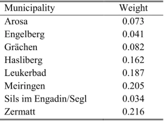
only using all pre-treatment outcomes as predictors. Using all pre-treatment outcome variables as separate predictors together with covariates, we get almost the same RMSPE as under the case with only all pre-treatment outcomes as predictors. Kaul et al. (2016) discuss that the use of all pre-treatment outcomes as predictors renders all covariates irrelevant. Ignoring truly influential covariates for future values of the outcome could cause a potential bias of the estimated treatment effect. Ignored observed covariates are not different from unobserved confounders. According to Abadie, Diamond, and Hainmueller (2010) is the SCM asymptotically unbiased even in the presence of unobserved covariates. Thus, according to Kaul et al. (2016) optimizing only the fit with respect to many lags of the pre-treatment outcome may to some part be beneficial. Considering our RMSPEs, we assume that our present covariates are not truly influential. Based on the discussion of Kaul et al. (2016) we do not use both, covariates and all pre-treatment outcomes. We only use pre-treatment outcomes as predictors for constructing our synthetic Saas-Fee and assume that we take more care of unobserved confounders. Table 2 shows the weights of each control municipality with a weight higher than zero. All other 97 communities get a weight of zero. The weights presented in Table 2 indicate that the trends of the residuals of domestic overnight stays in Saas-Fee in the pre-treatment period are best represented by a combination of Arosa, Engelberg, Grächen, Leukerbad, Hasliberg, Meiringen, Sils im Engadin/Segl and Zermatt. Zermatt gets the highest weight (0.216). It is a municipality close to Saas-Fee. It takes about 45 minutes to drive from Zermatt to Saas-Fee (according to Google Maps). Thus, the price discount in Saas-Fee might make overnight stays in Zermatt more attractive as well. If this is the case, the value for the domestic overnight stays of the synthetic Saas-Fee might be overestimated. Therefore, the effect of the discount might be even larger. On the other hand, the price discount could cause a cannibalization and ski destinations near to Saas-Fee would suffer from the price discount. We will consider this two spill over possibilities in section 4.3 in detail.
Table 2: Municipality weights for the synthetic Saas-Fee
Municipality Weight Arosa 0.073 Engelberg 0.041 Grächen 0.082 Hasliberg 0.162 Leukerbad 0.187 Meiringen 0.205 Sils im Engadin/Segl 0.034 Zermatt 0.216
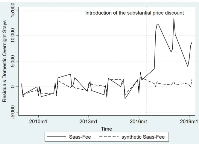
Graph 1 plots the residuals of domestic overnight stays for Saas-Fee and its synthetic counterpart during January 2009 and March 2018. As can easily be observed, the two trajectories track close in the entire period previous to the discount.10 This suggests, that the synthetic Saas-Fee provides a sensible
approximation to the number of residual overnight stays that would have been booked in Saas-Fee in the absence of the price discount.
10 See also table in the appendix with the numbers of the pre-treatment period’s outcome path form Saas-Fee and
9
Graph 1: Trends in residuals of domestic overnight stays: Saas-Fee vs. synthetic Saas-Fee
To estimate the effect of the price discount on the residuals of domestic overnight stays in Saas-Fee, we compare the differences of residuals of domestic overnight stays based on the seasonality of the pre-treatment periods in Saas-Fee and its synthetic counterpart in the post-intervention period. Regarding Graph 1, the two lines diverge after the introduction of the massive price discount. While the two lines have a common trend before the intervention, Saas-Fee has an obvious upward trend in the post-treatment period. The discrepancy in the residuals of domestic overnight stays suggests a large positive effect of the massive price discount on domestic overnight stays. The monthly impacts for the winter months in residuals of domestic overnight stays between Saas-Fee and its synthetic counterpart are substantial. Further, we see that the massive price discount has a large effect on domestic overnight stays. That are about 8’000 additional overnight stays in average per month in the municipality of Saas-Fee. The key results are presented in Table 3.
Table 3: Gap between overnight stays in Saas-Fee and the synthetic Saas-Fee in average (rounded) Per month 8’000 Per year 32’000 December 4’000 January 8’000 February 11’000 March 10’000
Before we discuss the results in more detail in section 4.3, we first evaluate the statistical inference of the overall effect in the next section.
10
4.2 Statistical Inference about the Effect of the Price Discount
To evaluate the significance of our estimates we question whether our results could be driven entirely at random. In this section, we therefore perform a series of placebo studies that confirm that our estimated effects for Saas-Fee are relatively large. We do so by conducting placebo tests on all municipalities in the donor pool. Then, we compare the distribution of the estimates that we obtain of the municipalities in the donor pool to the estimates of Saas-Fee. How often would we obtain results of the magnitude of our estimated effect if we had chosen a municipality at random? If the placebo studies create gaps of magnitude similar to the one estimated for Saas-Fee, then our interpretation is that our analysis does not provide significant evidence for a positive effect of the massive discount on the residuals of domestic overnight stays in Saas-Fee. However, if on the other hand the placebo studies show that the gap estimated for Saas-Fee is unusually large relative to the gaps for the municipalities that did not implement a large-scale season ticket discount program, then our interpretation is that our analysis provides significant evidence for a positive effect of the price discount on domestic overnight stays in Saas-Fee.
Graph 2 displays the results for the placebo tests. The grey lines represent the placebos; meaning, they show the difference between the residuals of domestic overnight stays of each municipality in the donor pool and its synthetic counterpart. The black line shows the gap estimated for Saas-Fee. As Graph 2 shows, the estimated gap for Saas-Fee in the post-treatment period is unusually large relative to the distribution of the gaps for the municipalities in the donor pool.
Graph 2: Distribution of placebo tests of 105 control municipalities and Saas-Fee
By estimating our “in-place” placebo effects we get two meaningful p-values. The first p-value amounts to 0.01. The p-value is constructed by the proportion of effects from the donor units that have a post-treatment RMSPE at least as large as the treated Saas-Fee. That is, one unit out of the 105 donor units
11
have a higher post-treatment RMSPE than Saas-Fee (1/105 = 0.0095). Graph 2 suggests some outliers which already have a high pre-treatment RMSPE. Therefore, we further calculate the proportion of placebos that have a ration of post-treatment RMSPE over pre-treatment RMSPE at least as large as the treated unit. This ratio amount to 0.019 (2/105 = 0.019). We have the two communities with a higher ratio of post-treatment RMSPE over pre-treatment RMSPE. Interestingly, one municipality is Annieviers. This community has been influenced by its new pricing strategy introduced for the winter season 2017/18. Since then, Anniviers cooperates with other ski resorts and introduced a cheap season ticket. Concluding our low p-values, the positive effect on residuals of domestic overnight stays in Saas-Fee is highly significant.
4.3 Discussion and General Findings
In this section, we show how to assess the assumptions presented in section 2.4 of the synthetic control method in a tourism destinations’ policy. We close the section by debating the causal effects of the price discount on tourism demand in Saas-Fee.
The first assumption is already graphically assessed in section 4.1. It is shown that Saas-Fee and its synthetic counterpart are almost similar in the entire period previous to the discount. As mentioned above, we second assume that the causing factor, the price discount, does not affect the control units. There are several ways, in which the assumption could be violated. The first option is, that the massive price discount causes an increase in overnight stays in municipalities near Saas-Fee. To control for this we discard two municipalities close to Saas-Fee from the donor pool (see section 3). As discussed above considering the municipality Zermatt, we would underestimate in this case the effect of the massive price discount. In example the promotion of the price discount of Saas-Fee would in this case have positive effects on overnight stays in mountain municipalities other than Saas-Fee. On the other hand, the price discount could cause a cannibalization. Ski destinations near to Saas-Fee would suffer under the massive price discount (also discussed by Falk and Scaglione 2018). If this would be the case, we would overestimate the effect of the massive price discount by giving weights to municipalities near Saas-Fee. As shown above, we give weights to the municipalities Grächen, Leukerbad and Zermatt. As Saas-Fee, these are municipalities of Canton Valais. Therefore, we also estimated the effects without municipalities of the Canton Valais in the donor pool. We got more or less similar results (about 7’000 additional overnight stays per month) and thus we only assume a marginal cannibalization in the ski destinations of this canton by the introduction of the price discount. Third, we assume that there exist no external shocks affecting the outcome of the control units. Other ski areas in Switzerland reacted to the descending demand with different price strategies (discounts, cooperation, dynamic pricing). These strategies could arise as an externa shock. Our conclusion from the qualitative consideration of these strategies is that these strategies are not as impressive as the discount in Saas-Fee. Therefore, we do not assume that the price strategies different to the strategy of Saas-Fee have triggered the same effect as the discount in Saas-Fee (no external shock on our control units). If this had been the case, we would underestimate the effect of the price discount in Saas-Fee.
Our results suggest causal effects of the price discount on domestic overnight stays in Saas-Fee. Our estimates suggest that the massive price discount has a large average effect of about 32’000 additional domestic overnight stays, our proxy for touristic demand, per winter season in the months December to March. The causal effect in the season 2018/19 is the lowest with 24’000 overnight stays. The average effect of 32’000 overnight stays amounts to 38% of the domestic overnight stays in the winter season 2015/16 in the municipality Saas-Fee, the season before the introduction of the price discount. Our result of 32’000 additional domestic overnight stays per winter seasons (2016/17, 2017/18 and 2018/19) is a little bit lower than the result of Falk and Scaglione (2018), who estimated the treatment effect in the
12
2016/17 winter season to be 48% for the winter sport destination of Saas-Fee. In addition to comparing the different seasons, thanks to our monthly-approach we are able to differentiate between the effects on a monthly basis. This can be a valuable piece of information for a destination with regard its price policy. For example, there may exist differences in monthly price elasticity of demand. The causal effect is greatest in February with an average effect of 11’000 additional overnight stays. On the other hand, the average effect is smallest in December with 4’000 additional overnight stays. Our results stay robust when we perform placebo studies. The p-values presented above are far below 5%, a test level typically used in conventional test of statistical significance. Based on the value creation study of the HES-SO Wallis (2016) about the canton of Valais, a hotel guest spends CHF 210 per overnight stay in a destination. The hotel guests spend money on accommodation, meals, transportation, leisure activities, local shopping and other expenses. About half of this relates to preliminary work.11 Thus, we get a direct
added value of about CHF 10 million in the municipality of Saas-Fee over the three winter seasons. We assume that with this amount we strongly underestimate the total value added for the destination of Saas-Fee. We do not consider the municipalities Saas-Grund and Saas-Almagell (both communities are part of the destination of Saas-Fee), the months of November and April, holiday flats, daily visitors and the indirect added value. Consequently, we assume that the price discount generated remarkable additional demand of tourism in the whole destination of Saas-Fee. Because we also estimated the effect excluding all municipalities of Canton Valais in the donor pool and got similar results, we assume that the price discount did not simply took demand form other destinations. Thus, we consider the price strategy of Saas-Fee as a success for the destination from a regional economy perspective. However, the mountain railways in Saas-Fee have decided to raise their ski pass prices after three years of low prices. From our opinion this does not necessarily have to be due to the fact that the price discount did not trigger any additional demand. This is more due to the fact that the mountain railways did not meet their needs and benefited from the rising demand to compensate for their loss of revenue caused by the discount. This decision could therefore be based on two reasons. First, it might be that the stakeholders in Saas-Fee did not sufficiently compensate the mountain railways for their investments. Secondly, the mountain railways were not vertically integrated enough (e.g. by owning hotels) to benefit from the increasing demand in business other than ski passes.
5 Conclusion
We apply the synthetic control method in order to analyse the causal effect of the introduction of a substantial price discount of the Swiss Alpine destination Saas-Fee. We use a data-driven procedure to construct such an appropriate synthetic Saas-Fee, which represents a comparison that excludes the treatment. Our synthetic Saas-Fee represents Saas-Fee better than a single comparison unit. We overcome the risk of choosing an inappropriate comparison, which might lead to erroneous conclusions. We discuss the assumptions of the synthetic control method and compare them to the difference-in-difference (DID) approach. Further, we show how to assess the assumptions of the synthetic control method in the context of a tourism destinations’ policy. Finally, we debate the causal effects of the price discount on tourism demand in Saas-Fee.
The empirical comparisons of tourism policy play an important role both in research as well as for tourism organizers and governments in order to document the success of their measures. The synthetic control method serves as an appropriate and promising research approach in order to compare and contrast the effects after changing system attributes. Our paper enriches the literature of tourism policy
13
comparisons. Wider applications of the SCM in the context of tourism will help scholars and practitioners to better understand the method its limitations and strengths. Further, the method might also fit to estimate the effect of economic or terroristic crises on tourism demand (Avraham 2015; Jin, Qu, and Bao 2019; Okumus, Altinay, and Arasli 2005). The use alongside or even the combination (see i.e. Arkhangelsky et al. 2019) of the SCM with the DID approach could help researchers in this understanding in further tourism research.
References
Abadie, Alberto, Alexis Diamond, and Jens Hainmueller. 2010. “Synthetic Control Methods
for Comparative Case Studies: Estimating the Effect of California’s Tobacco Control
Program.” Journal of the American Statistical Association 105(490): 493–505.
———. 2015. “Comparative Politics and the Synthetic Control Method.” American Journal of
Political Science 59(2): 495–510.
Abadie, Alberto, and Javier Gardeazabal. 2003. “The Economic Costs of Conflict: A Case
Study of the Basque Country.” The American Economic Review 93(1): 113–32.
Arkhangelsky, Dmitry et al. 2019. “Synthetic Difference In Differences.”
http://www.nber.org/papers/w25532.pdf.
Athey, Susan, and Guido W. Imbens. 2017. “The State of Applied Econometrics: Causality and
Policy Evaluation.” Journal of Economic Perspectives 31(2): 3–32.
Avraham, Eli. 2015. “Destination Image Repair during Crisis: Attracting Tourism during the
Arab Spring Uprisings.” Tourism Management 47: 224–32.
Becerra, Manuel, Juan Santaló, and Rosario Silva. 2013. “Being Better vs. Being Different:
Differentiation, Competition, and Pricing Strategies in the Spanish Hotel Industry.”
Tourism Management 34: 71–79.
Ben-Michael, Eli, Avi Feller, and Jesse Rothstein. 2018. “The Augmented Synthetic Control
Method.” (November). http://arxiv.org/abs/1811.04170.
Biagi, Bianca, Maria Giovanna Brandano, and Manuela Pulina. 2017. “Tourism Taxation: A
Synthetic Control Method for Policy Evaluation.” International Journal of Tourism
Research 19(5): 505–14.
Bouttell, Janet et al. 2018. “Synthetic Control Methodology as a Tool for Evaluating
Population-Level Health Interventions.” Journal of Epidemiology and Community Health
72(8): 673–78.
Castillo, Victoria, Lucas Figal Garone, Alessandro Maffioli, and Lina Salazar. 2017. “The
Causal Effects of Regional Industrial Policies on Employment: A Synthetic Control
Approach.” Regional Science and Urban Economics 67(August): 25–41.
Cavallo, Eduardo, Sebastian Galiani, Ilan Noy, and Juan Pantano. 2013. “Natural Disasters and
Economic Growth.” The Review of Economics and Statistics 95: 1549–61.
Falk, Martin, and Miriam Scaglione. 2018. “Effects of Ski Lift Ticket Discounts on Local
Tourism Demand.” Tourism Review 73(4): 480–91.
Gago, Alberto, Xavier Labandeira, Fidel Picos, and Miguel Rodríguez. 2009. “Specific and
General Taxation of Tourism Activities. Evidence from Spain.” Tourism Management
30(3): 381–92.
14
https://www.vs.ch/documents/303730/740705/Wertschopfung+des+Tourismus+im+Wall
is+2014/c68026fd-5633-41e5-bb89-fe9646496a56.
Islam, Muhammad Q. 2019. “Local Development Effect of Sports Facilities and Sports Teams:
Case Studies Using Synthetic Control Method.” Journal of Sports Economics 20(2): 242–
60.
Jin, Xin (Cathy), Mingya Qu, and Jigang Bao. 2019. “Impact of Crisis Events on Chinese
Outbound Tourist Flow: A Framework for Post-Events Growth.” Tourism Management
74(April): 334–44.
Kaul, Ashok, Stefan Klößner, Gregor Pfeifer, and Manuel Schieler. 2016. “Synthetic Control
Methods: Never Use All Pre-Intervention Outcomes Together With Covariates.” (83790).
https://mpra.ub.uni-muenchen.de/83790/1/MPRA_paper_83790.pdf.
Khadaroo, Jameel, and Boopen Seetanah. 2007. “Transport Infrastructure and Tourism
Development.” Annals of Tourism Research 34(4): 1021–32.
Naude, Willem A., and Andrea Saayman. 2005. “Determinants of Tourist Arrivals in Africa :”
Tourism Economics 11(3): 365–91.
Nusair, Khaldoon, Hae Jin Yoon, Sandra Naipaul, and H. G. Parsa. 2010. “Effect of Price
Discount Frames and Levels on Consumers’ Perceptions in Low-End Service Industries.”
International Journal of Contemporary Hospitality Management 22(6): 814–35.
Okumus, Fevzi, Mehmet Altinay, and Huseyin Arasli. 2005. “The Impact of Turkey’s
Economic Crisis of February 2001 on the Tourism Industry in Northern Cyprus.” Tourism
Management 26(1): 95–104.
Ponjan, Pathomdanai, and Nipawan Thirawat. 2016. “Impacts of Thailand’s Tourism Tax Cut:
A CGE Analysis.” Annals of Tourism Research 61: 45–62.
Rütter, Heinz, and Ursula Rütter-Fischbacher. 2016. Wertschöpfungs- und
Beschäftigungswirkung
im
ländlichen
und
alpinen Tourismus.
https://regiosuisse.ch/sites/default/files/2016-10/Studie_Berggebiete_Ruetter.pdf.
Saha, Shrabani, and Ghialy Yap. 2014. “The Moderation Effects of Political Instability and
Terrorism on Tourism Development: A Cross-Country Panel Analysis.” Journal of Travel
Research 53(4): 509–21.
Seilbahnen Schweiz, Seilbahnen. 2017. “Fakten und Zahlen zur Schweizer Seilbahnbranche.”
www.seilbahnen.org.
Stettler, Juerg, Myrta Zemp, and Angela Steffen. 2015. “Alpine Smart Tourism Destination:
Überblick über den Smart Tourism Ansatz sowie über geplante Initiativen.” ITW Working
Paper (May): 1–32.
Zhang, Jiekuan, and Yan Zhang. 2018. “Carbon Tax, Tourism CO 2 Emissions and Economic
Welfare.” Annals of Tourism Research 69(August 2017): 18–30.
15
Appendix
The municipalities in the control group are: Adelboden, Aeschi bei Spiez, Airolo, Amden, Andermatt, Anniviers (Valais), Arosa, Avers, Ayent (Valais), Bad Ragaz, Bagnes (Valais), Beatenberg, Beckenried, Bellwald, Bever, Bex, Blatten (Valais), Breil/Brigels, Brienz (BE), Brig-Glis (Valais), Celerina/Schlarigna, Chalais (Valais), Champéry (Valais), Chur, Churwalden, Château-d'Oex, Châtel-Saint-Denis, Davos, Disentis/Mustér, Emmetten, Engelberg, Evolène (Valais), Faido, Fiesch (Valais), Flims, Flums, Flühli, Frutigen, Gersau, Grindelwald, Gruyères, Grächen (Valais), Hasliberg, Innertkirchen, Interlaken, Kandersteg, Kerns, Klosters-Serneus, La Punt-Chamues-ch, Laax, Lauterbrunnen, Lenk, Lens (Valais), Leukerbad (Valais), Leysin, Leytron (Valais), Meiringen, Morschach, Mörel-Filet (Valais), Naters (Valais), Nendaz (Valais), Obergoms (Valais), Ollon, Ormont-Dessous, Ormont-Dessus, Orsières (Valais), Plaffeien, Pontresina, Quarten, Realp (Valais), Riddes, Ried-Brig (Valais), Riederalp (Valais), Saanen, Samedan, Samnaun, Schangnau, Schiers, Schwende, Schwyz, Scuol, Sigriswil, Sils im Engadin/Segl, Silvaplana, Sion (Valais), Splügen, St-Moritz, Tschappina, Tujetsch, Täsch, Val Müstair, Val-d'Illiez (Valais), Vals, Vaz/Obervaz, Vilters-Wangs, Vitznau, Walenstadt, Weggis, Wilderswil, Wildhaus-Alt St-Johann, Wolfenschiessen, Zermatt (Valais), Zernez, Zuoz and Zweisimmen.
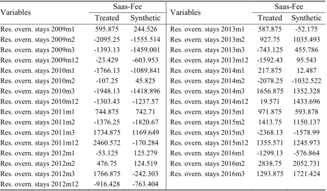
Table 4: Pre-treatment characteristics Saas-Fee and synthetic Saas-Fee
Variables Treated Synthetic Saas-Fee Variables Treated Synthetic Saas-Fee
Res. overn. stays 2009m1 595.875 244.526 Res. overn. stays 2013m1 587.875 -52.175 Res. overn. stays 2009m2 -2095.25 -1555.514 Res. overn. stays 2013m2 927.75 1035.493 Res. overn. stays 2009m3 -1393.13 -1459.001 Res. overn. stays 2013m3 -743.125 455.786 Res. overn. stays 2009m12 -23.429 -603.953 Res. overn. stays 2013m12 -1592.43 95.543 Res. overn. stays 2010m1 -1766.13 -1089.841 Res. overn. stays 2014m1 217.875 12.487 Res. overn. stays 2010m2 -107.25 45.825 Res. overn. stays 2014m2 -2078.25 -1032.522 Res. overn. stays 2010m3 -1948.13 -1418.896 Res. overn. stays 2014m3 1656.875 1352.328 Res. overn. stays 2010m12 -1303.43 -1237.57 Res. overn. stays 2014m12 19.571 1433.696 Res. overn. stays 2011m1 744.875 742.71 Res. overn. stays 2015m1 971.875 593.878 Res. overn. stays 2011m2 -1376.25 -1820.67 Res. overn. stays 2015m2 1413.75 1150.137 Res. overn. stays 2011m3 1734.875 1169.649 Res. overn. stays 2015m3 -2368.13 -1578.99 Res. overn. stays 2011m12 2460.572 -170.284 Res. overn. stays 2015m12 1355.571 1245.973 Res. overn. stays 2012m1 -53.125 125.279 Res. overn. stays 2016m1 -1299.13 -576.864 Res. overn. stays 2012m2 476.75 124.519 Res. overn. stays 2016m2 2838.75 2052.731 Res. overn. stays 2012m3 1766.875 -242.303 Res. overn. stays 2016m3 1293.875 1721.424 Res. overn. stays 2012m12 -916.428 -763.404
16
Table 5: Descriptive Statistics Covariates
Variable Mean SD Minimum Maximum
Ski lifts 24.06 31.93 1 216
Skiruns in km 103.89 129.20 1 650 Elevation of lift station (peak) 2483.96 557.41 1’365 3’899 Fast Licensed Lifts 7.71 6.79 0 25 Dist. Swiss city car (minutes) 87.44 38.08 20 166 Dist. Swiss city public tra. (minutes) 112.70 46.83 34 254 Hotels per municipality 12.70 12.62 2.67 96.92
Author
Hannes WALLIMANN
University of Fribourg, Department of Economics, Ph.D. student
Lucerne University of Applied Sciences and Arts, Institute of Tourism, Research Associate
Phone: +41 41 228 99 30; Email: hannes.wallimann@hslu.ch; Website: https://www.hslu.ch/en/lucerne-university-of-applied-sciences-and-arts/about-us/people-finder/profile/?pid=4076
Bd de Pérolles 90, CH-1700 Fribourg Tél.: +41 (0) 26 300 82 00
decanat-ses@unifr.ch www.unifr.ch/ses Université de Fribourg, Suisse, Faculté des sciences économiques et sociales
Universität Freiburg, Schweiz, Wirtschafts- und sozialwissenschaftliche Fakultät University of Fribourg, Switzerland, Faculty of Economics and Social Sciences
Working Papers SES collection
Abstract
The synthetic control method serves as an appropriate and promising approach to do quantitative comparison
research. However, the method is rarely used in the context of tourism. We fill this research gap by applying the
method to the case of a Swiss mountain destination. Alpine tourist destinations have suffered from a declining demand
in the last decade. Fewer tourist visit ski resorts. Consequently, the tourism industry in these destinations is under
pressure to seek for solutions to face this falling demand. Saas-Fee, a Swiss mountain destination particularly hard
hit by the decline of visitors has come up with an innovative offer: A substantial price discount on ski passes. In this
present study, we aim to estimate the causal effect of the price discount in Saas-Fee. We adopt the synthetic control
method to analyze the impact of the destinations’ policy on tourism demand. Further, we perform placebo tests on all
units in our donor pool to evaluate the significance our results. Finally, we show how to assess the assumptions of the
synthetic control method in the context of tourism.
Citation proposal
Hannes Wallimann. 2019. «A Substantial Discount on Ski Passes: A Synthetic Control Analysis». Working Papers SES 507, Faculty of Economics and Social Sciences, University of Fribourg (Switzerland)
Jel Classification
C21, Z32, Z38
Keywords
Tourism policy evaluation; Synthetic control method; Swiss Alps; Price discount.
Last published
500 Huber M.: A review of causal mediation analysis for assessing direct and indirect treatment effects. 2019
501 Arifine G., Felix R., Furrer O.: Multi-Brand Loyalty in Consumer Markets: A Qualitatively-Driven Mixed Methods Approach; 2019
502 Andre P., Delesalle E., Dumas C.: Returns to farm child labor in Tanzania; 2019 503 De La Rupelle M., Dumas C.: Health consequences of sterilizations; 2019 504 Huber M.: An introduction to flexible methods for policy evaluation; 2019
505 Schünemann J., Strulik H., Trimborn T.: Medical and Nursery Care with Endogenous Health and Longevity; 2019
506 Fernandes A., Huber M., Plaza C.: The Effects of Gender and Parental Occupation in the Apprenticeship Market: An Experimental Evaluation; 2019
Catalogue and download links
http://www.unifr.ch/ses/wp
http://doc.rero.ch/collection/WORKING_PAPERS_SES