Assessments of long-term uranium supply availability

ASSESSMENTS OF LONG-TERM URANIUM SUPPLY AVAILABILITY by

Daniel R. Zaterman

SUBMITTED TO THE DEPARTMENT OF NUCLEAR SCIENCE AND ENGINEERING

IN PARTIAL FULFILLMENT OF THE REQUIREMENTS FOR THE DEGREE OF BACHELOR OF SCIENCE IN NUCLEAR SCIENCE AND ENGINEERING

AT THE

MASSACHUSETTS INSTITUTE OF TECHNOLOGY MASACHUSE, S iSTTUTE

MAY 8, 2009 AUG

1

Daniel R. Zaterman. All rights reserved.

LIBRARIES

The author hereby grants to MIT permission to reproduce and to distribute publicly paper and electronic copies of this thesis document in whole or in part.

Signature of Author:

Certified by:

Accepted by: .

L

/ Daniel R. Zaterman

epartmentNucl Science and Engineering May 8, 2009

Richard K. Lester Director, MIT Industrial Performance Center

/ Professor, Nuclear Science and Engineering

S. Kim Molvig

Associate Professor, Nuclear Science and Engineering Chair, NSE Committee for Undergraduate Education

ASSESSMENTS OF LONG-TERM URANIUM SUPPLY AVAILABILITY By

Daniel R. Zaterman

Submitted to the Department of Nuclear Science and Engineering on May 8, 2009 In Partial Fulfillment of the Requirements for the Degree of

Bachelor of Science in Nuclear Science and Engineering

ABSTRACT

The future viability of nuclear power will depend on the long-term availability of uranium. A two-form uranium supply model was used to estimate the date at which peak production will occur. The model assumes a constant annual rate of production growth to the peak, and a fixed reserves-to-production ratio thereafter. For mid-range assumptions of reserves and production growth rates, production is estimated to peak in 2076. Additionally, a net-present-value (NPV) analysis was used to model annual uranium exploration investment as a function of historical discovery costs; historical discovery, development, and production lifetimes; spot uranium prices; and credit availability. When back-tested over the past 30 years, the model successfully 'predicted' annual investment rates. Finally, multiples analysis was applied to estimate

Australia's undiscovered and speculative resources, which were found to be 447,500 tU and 2,237,400 tU, respectively. The results of these analyses suggest that higher prices, increased exploration, and the use of non-conventional sources of uranium can provide plentiful supplies for at least the next century.

Thesis Supervisor: Richard Lester

Director, MIT Industrial Performance Center Professor, Nuclear Science and Engineering

Table of Contents

1. Introduction 4

2. Theory 18

3. Methods and Assumptions 21

4. Comparison of Uranium Production Peak to Other Resource Markets 25 5. Development of Model for Uranium Exploration Expenditure 34 6. EAR-II and Speculative Resource Estimates for Australia 46

7. Conclusions 49

1. Introduction

Since the initial development of commercial nuclear power in the 1960s, the global demand for uranium, the primary fuel for nuclear reactors, has increased steadily. In 2004, the

annual demand for uranium was approximately 60,000 tons per year (IAEA, 2001). As global concerns about the environment and the sustainability of current energy sources increase, many analysts predict a nuclear renaissance. As part of this rebirth, it is possible that hundreds of new plants could come online over the next few decades. A number of demand analyses have been performed, and the IAEA's mid-range demand assumption predicts that by 2050 demand could reach 177,000 tons/year (IAEA, 2001).

In nature, uranium ore exists in the chemical form U308. Natural uranium contains 0.7%

U-235, the fissile isotope of uranium, and the remainder is U-238. Although most nuclear reactors burn low-enriched uranium fuel (3-5% concentration ofU-235) in the chemical form UO2, uranium prices are typically quoted in dollars per kilogram of the metal.

Like other elements on this planet, there is a finite supply of uranium available to be used as fuel. The global uranium supply is subdivided into two categories: primary and secondary

supply. Primary supply, which comprises newly mined and processed uranium, is broken categorized into four groups by the IAEA: uranium produced in the Commonwealth of

Independent States (CIS), small governmental programs, China, and market-based production. Primary resources are further categorized in Uranium Resources Production and Demand the authoritative report produced every two years jointly by the Nuclear Energy Agency of the OECD and the IAEA (and popularly known at the "Red Book"), into reasonably assured resources (RAR), estimated additional resources category 1 (EAR-I), lower probability

these categories, resources are further broken down by the cost of production. RAR and EAR-I estimates account for mining and milling losses; however, EAR-II and SR estimates are reported as in situ quantities, and do not account for these losses.

Secondary supply comprises high enriched uranium (HEU), natural and low enriched uranium (LEU) inventories, mixed oxide fuel (MOX), reprocessed uranium (RepU), and re-enriched depleted uranium (tails) (IAEA, 2001). Currently, secondary supply (mostly from blending down surplus high-enriched uranium from the Russian nuclear weapons stockpile) provides over 40% of annual demand (IAEA, 2001). Secondary supplies, however, are not

growing and consequently the IAEA believes that by 2025 they will only contribute between 4 and 6% of the total (IAEA, 2001). Today, over 50% of the world's primary uranium comes from Canada, Australia, and Kazakhstan. Canada is the largest producer; however, it is possible that Australia will surpass it in the near future (HOR, 2006).

In addition to primary and secondary resources, there are also unconventional sources of uranium. These include the uranium found in seawater as well as phosphorite, black shale, and lignite deposits (IAEA, 2001). Unconventional resources are typically characterized by high costs of production and in many cases commercial production methods are unproven. Japanese researchers have noted that the world's oceans, which contain approximately 3 ppb uranium, could provide a nearly limitless source of uranium (Tamada et al., 2006). They have

demonstrated that absorbent membranes submerged in the ocean could be used to produce uranium at an estimated cost of $240/Kg U (Tamada et al., 2006). Although the production costs

are significantly higher than those of conventional uranium production, this method could in principle make available an additional 4 billion tons of uranium.

A recent IAEA study estimated the amount of uranium from primary and secondary supplies that would be available through 2050. The study used a mid-range demand case that assumed medium economic growth, government policies supporting nuclear power, and low energy demand growth but continued development of nuclear power worldwide (IAEA, 2001). The study showed that by 2040, secondary supplies and market based production of RAR through EAR-II would fall short of annual demand (IAEA, 2001). In addition, the study showed that the size of the shortfall would continue to grow during the following decade (IAEA, 2001). The implication of this observation is that speculative and unconventional resources will be needed in the future in order to fulfill the world's annual uranium demand.

In order to understand the significance of this result, uranium must be compared to other resource markets. Oil and copper are both natural resources of finite supply on this planet. Multiple studies have suggested that peak production for oil and for copper could occur within the next decade based on different assumptions for the supply, demand, exploration, and future production capacity.

The taxonomy for crude oil resources is different from that of uranium and thus must first be clarified. There are four basic categories of oil reserves: proved, probable, possible, and unproved. Proved reserves have a median confidence level of 90% of being produced and are referred to as lP. Probable (2P) and possible reserves (3P) have confidence levels of 50% and

10%, respectively. Unproved resources are those that have not been substantiated but are mostly considered for exploration by oil companies. Although there is no perfect analog between uranium and crude resource taxonomies, RAR and 1P are most comparable, as are EAR-I and 2P, EAR-II and 3P, and speculative and unproven resources.

The crude oil market is among the most studied resource markets due to its critical role in energy security across the globe. Various government entities, consultancies, and private

companies have analyzed oil supply. Recently, the International Energy Agency published the World Energy Outlook 2008 in which they suggested that peak crude production from fields currently producing and fields yet to be developed could occur as early 2015 (IEA, 2008). The basis for these assumptions was a field-by-field study of 800 currently producing sites. From these analyses, it was estimated that the rate of decline in output will increase from 6.7% annually to 8.6% by 2030 (IEA, 2008). Even in a scenario of zero demand growth, 45 million barrels per day (mb/d) of additional production would be needed to offset the declines of existing wells (IEA, 2008). Using the IEA's demand growth predictions, an additional 64 mb/d of

capacity, approximately six times Saudi Arabia's current annual production, would be required by 2030. In order to meet this demand, undiscovered fields, enhanced oil recovery (EOR) at

existing fields, non-conventional oil such as tar sands, and natural gas oils would all need to be utilized (IEA, 2008). The EA estimates that -$5 trillion dollars would need to be spent on exploration over the next 21 years to tap those supplies.

In 2004, researchers at the U.S. Energy Information Administration (Wood et al., 2004) made their own predictions for future oil supply using a slightly different method. Their study assumed a fixed stock of conventionally-reservoired crude oil. To estimate this quantity, they consulted the results of a 2000 USGS survey of world supply, which was conducted by a team of 40 geoscientists over a period of 5 years using scientific methods to analyze the world's most prolific wells (Wood et al., 2004). With this estimate of ultimately recoverable oil, and a margin of error, the EIA team modeled production between 2003 and the peak output year assuming a constant 2 percent annual growth rate over this period, the historical average. After peak

production, the decline was modeled by assuming a constant reserve-to-production ratio (R/P) of 10. Using this methodology the EIA predicted peak production in 2037 and near-depletion by 2100 (Wood et al., 2004). A number of sensitivity analyses were performed to see how changes in different variables would affect the estimated peak. Both the IEA and EIA studies suggest that non-conventional oil sources will have to provide significant supplies within the next 30 years if consumption is to continue at current levels or grow.

Unlike uranium and crude oil, currently-in-use copper can be melted down and reused. The earth's supply of copper is typically subdivided into ores in the lithosphere, copper

providing services or being recycled, and waste copper in landfills (Graedel et al., 2006). Copper is classified as (1) 'reserves' -- copper that has been discovered and is currently economical to produce; (2) the 'reserve base', which includes copper that has been discovered but is not currently viable due to economics and technology, (3) 'resources', which are undiscovered but theoretically viable from an economic and technological standpoint, and the 'resource base', which consists of all of the earth's copper.

It is very important to consider that in any peak resource analysis, the only true fixed stock is the total resource base consisting of every atom of that material on this planet. By this measure, conventional and non-conventional resources alike must be accounted for, and no bounds on the production costs can be applied. The McKelvey diagram, shown in Figure 1.1

Identified Undiscovered

resources resources

Proved Inferred

conomic reserves reserves

0 (D E -Sub-economic _O . Increasing geological assurance

Figure 1.1 The McKelvey Diagram for the Relationship between Reserves and Resources (Skinner, 2001)

can be used to analyze the mineral resources, where the total fixed-stock is represented by the area of the entire diagram. The primary forces at work in this diagram are exploration, which can move undiscovered resources into reserves, and prices and technology which can expand the

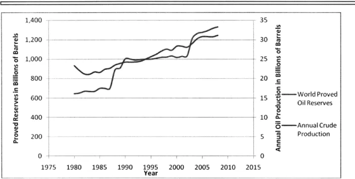
region of what is economic. Over time, production removes material from the resource region; however, it has also been shown that the amount of reserves is constantly being replenished if not increased over time. This has been demonstrated in the case of oil. In Figure 1.2, EIA

I I 1,400 - - ---.--. .- - - -- 355 0 2 t 800 - - - 20 0 600 . ... ... -- --- - - 15 " ,----World Proved S Oil Reserves 0 400 --- 10 --- Annual Crude 200 -- -- 5 Production 0 --- r--- --- --- - ---- ---- - 0 1975 1980 1985 1990 1995 2000 2005 2010 2015 Year

Figure 1.2 EIA estimates for world proved oil reserves and annual oil production over time (EIA, 2009)

estimates for the world's proved oil reserves are plotted with annual oil production. Despite increasing production, oil reserves are increasing suggesting that historically, undiscovered resources have evolved into higher assurance reserves, offsetting annual production. In the copper market, peak supply theories have also been suggested, although a less scientific methodology has been employed to describe the peak scenario. Graedel et al. analyzed copper production in North America over the 20h century, and concluded that of the 164 billion metric tons (Tg) of copper mined, 70 Tg remained in use (Graedel et al., 2006). They established that

170 kg of copper per capita were in use North America, and further concluded after reconciling with bottoms-up- analysis that developed nations such as the United States required -200 kg of

copper per capita for their technological and infrastructure needs (Graedel et al., 2006). After consulting USGS estimates for global porphyry (conventional) copper resource and accounting for non-porphyry copper they estimated that global copper resources were 1600 Tg (Graedel et al., 2006). They then argued that given an estimated global population of 10 billion by 2100,

1700 Tg would be required to bring the per-capita copper-in-use to North American levels. They asserted that in order for the rest of the world to develop post-industrial technological standards by 2050, there will not be enough copper available in the lithosphere to provide the average 200 kg/capita for an estimated population of 8.7 billion (Graedel et al., 2006). Graedel et al.'s theory suggests an alarming situation, although it has elicited several criticisms.

Researchers at the Pontificia Universidad Cat61lica in Chile have suggested that an opportunity cost model more accurately describes the copper market as opposed to the fixed-stock model suggested by Graedel et al. They first argue that copper needs are best quantified not as a per capita average, but rather as a more complicated function of technological innovation, population growth trends, income per capita, consumption preferences, opportunities for material substitution, and recycling (Tilton et al., 2007). They contend that the resource base is the only true fixed stock of copper, and not the resources that Graedel et al use in their assumptions (Tilton et al., 2007). They also contend that Graedel et al do not account for seabed copper, and propose that there is actually 3000 Tg of copper resources based on more recent estimates. They believe that because resource estimates have dramatically changed over the past 10 years,

assuming depletion based on a constantly fluctuating quantity is unreasonable (Tilton et al., 2007). Finally they argue that copper prices can simply rise in the long-term to make previously uneconomical copper viable, and continued exploration will convert undiscovered resources into reserves (Tilton et al., 2007).

Another important factor in uranium supply dynamics is investment in exploration. Since the early 1940's when nuclear energy was first discovered, exploration has yielded 3,338,300 tU of RAR and 2,130,600 tU of EAR-I producible for less than 130 $/kgU according to the 2007 Red Book survey (OECD, 2007). Global exploration expenditure has varied greatly with time as

shown in Figure 1.3. Figure 1.3 illustrates that from 1990 to 2004 exploration investment was

I

ooooo

o

Figure 1.3 2007 Red Book survey of global uranium exploration expense ($ 1000) as a function of time (OECD, 2007)

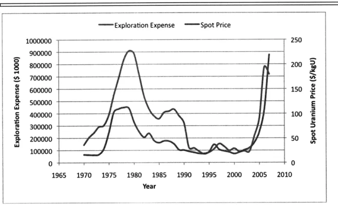
minimal as compared with historical averages. One explanation for this trend was weak uranium prices over that period as well as increased availability of uranium from secondary supplies. Figure 1.4 plots exploration annual exploration against spot uranium prices. At a superficial

-Exploration Expense -Spot Price 1000000 250 900000 8 800000 - 200 S700000 - -C 600000 150 S 500000 _E 400000 100 E 1 300000 ooo M 200000 50 C 100000 0 0 1965 1970 1975 1980 1985 1990 1995 2000 2005 2010 Year

Figure 1.4 Global uranium exploration expense ($ 1000) and uranium spot price ($/kgU) as function of time (OECD, 2007)

level. Figure 1.4 shows a strong correlation between spot price and exploration investment for the past 27 years; however, the relationship is more complicated. First, approximately 60-80% of

all uranium trades through long-term contracts as opposed to in the spot market. Long-term contracts typically range from 3-5 years and include a first delivery 24 months in the future (Roberts, 2009). Although there is no industry standard, these contracts typically contain price floors and caps, but include escalators to account for fluctuations in shorter term prices (Roberts, 2009). Therefore spot prices, reflecting -30% of total uranium transactions, are not necessarily a good indicator of the "price of uranium" (Roberts, 2009). Another consideration is that

investment in exploration is subject to the availability of financing (Roberts, 2009). Most private uranium miners are not heavily levered companies and finance exploration activity through a number of different methods. These options include bank lines of credit, project financing flow through, and in many cases equity private placements (Roberts, 2009). The availability of

financing options in the capital markets is critical for exploration to continue and thus should be accounted for. From the standpoint of uranium mining companies, the decision to invest in exploration is made with the intent of making a discovery and being able to generate revenue and a positive return on the investment. Therefore mining companies' expectations for times to discovery, times to production, and the production lifetime of a site are all factors in the decision of mining companies to explore. One of the objectives of this paper is to develop a model for the uranium exploration investment that is a function of uranium prices (spot and long term),

historical discovery costs, historical timing of mining operations, and the availability of financing.

It is important to study uranium exploration habits because the time between new exploration and production from a mine can be greater than ten years (Kee, 2007). Uranium mining, like other types of mining, is subject to significant licensing, zoning, environmental, and political risks. Most recently, the world's largest uranium producer, Cameco, faced significant setbacks at its Cigar Lake facility in Canada (Kee, 2007). This site, which at full-capacity will contribute upwards of 10 percent of the total global production, flooded in 2006, delaying commercial production beyond 2008 (Kee, 2007). Because accidents like this are inherent in primary uranium supply, it is necessary to maintain a continued flow of exploration and

development so as to mitigate the risk of mining and regulatory uncertainties but also to maintain steady production levels.

Another unique characteristic of uranium supply is that government regulation in many cases prohibits exploration, mining, and exportation. In Australia, for example, national

government limits on exportation, and state government restrictions on mining have caused underutilization of Australia's abundant supply of uranium. Currently only three mines (Ranger,

Olympic Dam, and Beverly) are producing uranium; however, Australia is expected to become the largest producer of uranium (HOR, 2006). Australia contains 38 percent of the world's low-cost, discovered resources (RAR + EAR-I), but has never published estimates for EAR-II or speculative resources (HOR, 2006). Since 1999, exploration investment in Australia has increased dramatically as reflected in Table 1.1. This increase is a reflection of increased Table 1.1 Australia Uranium Investment Since 1999 (OECD, 2007)

Year Exploration Expense

(AUD million) 1999 9.61 2000 7.59 2001 4.80 2002 5.34 2003 6.38 2004 13.96 2005 41.09 2006 80.70 2007 90.70

governmental support for exploration and opening uranium to exportation. Currently over 200 junior exploration companies, companies that do not generate revenue from any production but

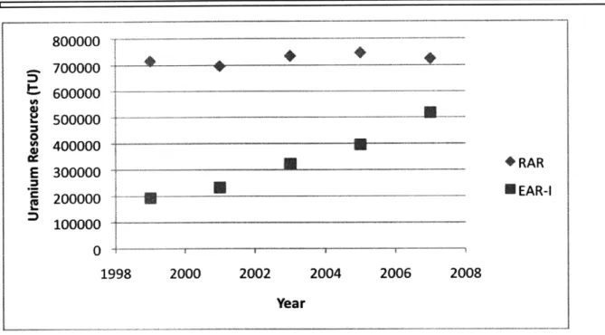
are simply financed to make discoveries, are operating within Australia. Although the increased investment in has not caused RAR estimates to change much with time, EAR-I estimates have grown dramatically year over year. Figure 1.5 illustrates this trend of increasing EAR-I

800000 700000 600000 500000 400000 300000 200000

i

Figure 1.5 RAR and EAR-I resource estimates for Australia since 1999 (OECD, 2007)

I I

estimates. Obviously, increased exploration has spurred increased expectations. As Australia trends toward becoming the world's largest uranium producer, it becomes important to try to quantify Australia's EAR-II and speculative resources to gauge what impact they will have on global estimates and thus on the future supply/demand dynamics for Uranium. Because no formal analyses have been performed by Australian officials, a multiple analysis can be

performed to estimate these values. By taking the ratio of SR + EAR-II to RAR + EAR-I in other countries with high concentrations of low-cost uranium, an appropriate multiple can be found. Multiplication by this factor should provide reasonable estimates for these resources in Australia, which can be studied in the context of global estimates.

Through these studies, I expect to show that the long-term uranium supply situation is far less grave then many reports have suggested, and that higher prices, increased exploration, and the use of non-conventional sources of uranium can provide plentiful supply for at least the next century. Furthermore, I hope to show that uranium exploration investment can be modeled as a function of spot and long-term prices, historical development costs, discovery times, licensing

I I

periods, and production lifetimes. The success of this model can be defined in terms of back testing on historical data. Finally, this study should provide reasonable estimates for Australia's resources, and show that global estimates of RAR through SR are actually quite sensitive to these estimates.

2. Theory

Estimation of peak production or supply depletion for a given resource can be

approached through a variety of methods. At the core of the differences between these methods are different assumptions about the total quantity of resources available on earth. The EIA approached the problem of predicting peak oil by modeling production in functional forms. The first form is continued production growth at a fixed rate equal to the historical trend in annual production. The second form is production at a fixed ratio of production to reserves. Earlier models, such as the King Hubbert model, defined the decline in post-peak production as symmetrical to the buildup. The EIA analyzed post-peak production for individual wells in the United States, and concluded that production was best modeled as a fixed R/P ratio of 10 (Wood et al., 2004). Using the Canada as a model for the developed world, the R/P ratio was applied to global production. The integral of the two-form function, which accounts for the differences between pre-and post-peak production behavior, must equal the estimates for the total

conventional resources (RAR through SR). This method, which will be referred to as the EIA method, can be applied to uranium to evaluate its peak production date.

Another method of analyzing resource depletion is to take a fixed-stock approach. This method, which was applied by Graedel et al. to analyze the global supply of copper, is a very high-level form of analysis. In this model, global resources of a given mineral are taken to be a fixed stock. Next, the per capita resources-in-use are estimated for developed nations. By

assuming a global progression toward developed, post-industrial standards and estimating global population growth, the time by which the fixed supply of a resource will be completely used up can be predicted. After comparing uranium supply to copper and oil supplies, the next objective was to develop a model for uranium exploration expense. In order to describe this behavior of

uranium mining companies, the basics of the time-value of money and net present value must be considered. The basic concept behind this theory is that the value of a dollar in the present day is worth more than a dollar in the future. The present value (NPV) of future cash flows (FCF) can be defined according to the equation,

NPV = FCF, _(2.1)

where t represents the time in the future in years and r represents the discount rate in % / year. From the perspective of corporations, the discount rate reflects the cost of financing a project through equity or debt. The notion is that investors expect a specific return on investment for the risks associated with such an upfront expenditure. Because the goal of public companies is to maximize shareholder equity, the decision to invest in exploration must thus be evaluated from an NPV standpoint. Executives in the mining industry attest to the fact that every exploration project is evaluated differently due to the idiosyncrasies of different types of terrain, the availability of equipment, ore concentration, as well as many other factors. Despite these wide variations, the aggregate behavior of the entire uranium mining industry can be modeled based on historical data. One factor to consider is that exploration investment often results in no discovery. Therefore the return on every exploration dollar should be treated with an expectation value of discovery. Another way to represent this uncertainty is to evaluate historical discovery costs, which represent the total resources discovered plus those produced divided by the total investment. By using historical discovery costs, times to discovery, times to production,

production lifetime, average costs of production, revenue estimates derived from spot and long-term uranium prices, and appropriate discount rates which affect the availability of financing for mining companies, the NPV of an exploration project can be evaluated. Evaluating the NPVs for different periods in time, threshold NPVs for investment can be developed, and subsequently the

amount of investment can be defined as a function of the NPV. The final result will be a model for current and future exploration investment as function of the credit spreads and equity financing costs and market prices for uranium (spot and long-term).

Multiples analysis will also be used in this study. The theory behind this method is that the ratio of two values can be used to calculate an unknown value, if one of the values is known for a comparable entity. This type of analysis is often used in finance. In order to predict future stock prices, the price to earnings (P/E) ratio of comparable companies is often used. By

multiplying expected earnings of one company by the P/E ratio of the comparable company, a reasonable estimate for a company's future stock price can be derived. This method will be

similarly applied to estimate the EAR-II and SR of uranium in Australia, values that have never been formally evaluated. In the case of this study, the comparable nations from which the

multiplier of (SR+EAR-II)/ (RAR +EAR-I) will be derived are Canada and Kazakhstan. These are the first and third largest uranium producers and, like Australia, both countries' resources are primarily high-grade and producible at low cost.

3. Methods and Assumptions

The initial stage of this study involved extensive research of the uranium markets by consulting scholarly publications, Red Book resource assessments, government analyses of supply dynamics, and financial statements from uranium mining companies. Interviews with the executives from Dennison Mines, a mid-size international uranium mining company, provided

further details on the operations of industry participants. Having aggregated a mass of historical data and future predictions, the first component of this study was to investigate possible peak production timelines for uranium. To estimate this peak scenario, the EIA method was applied.

The most recent Red Book estimates for the RAR through SR were used to account for the total resources available. A factor of 0.8 was applied to the EAR-II and SR estimates to account for mining and milling losses. The growth rate for production up to the peak was taken as the average annual global production growth rate since 1945. The ratio of available production capacity to annual production was calculated using the average of this ratio for Canada from 1968 to the present. Because Canada is the world's largest uranium producer, its capacity utilization factor was seen as an appropriate ratio to apply to the rest of the world. Next, the production peak was approximated by combining the growth and constant R/P ratio decline models subject to the constraint of satisfying the estimate for the global conventional supply. Sensitivity analyses were then performed to see how changes in the estimated growth rate, total supply estimate, and the R/P ratio affected the predicted peak production rate.

The fixed-stock method was then applied to estimate when the world's uranium supply would be depleted. Again the total global supply was assumed to be the supply of conventional resources RAR through SR with a factor of .8 discounting the EAR-II and SR estimates. The per-capita annual uranium consumption-per-year was taken through analysis of the consumption in

France and the United States. France and the United States were chosen as the benchmarks due to their significant utilization of nuclear power at 80 and 20 percent, respectively. The per capita uranium requirements were approximated by calculating the uranium requirements for plants within each of the countries per year. These values were then divided by the most recent population estimates for those countries to calculate the per capita requirements. Consulting population growth estimates, the annual uranium requirements were calculated for future dates

assuming that per-capita needs had reached the levels of the United States and France. From these annual needs, the depletion date for the world's conventional uranium supply was estimated.

Next a model for exploration investment was developed. First, historical discovery costs (Cd) were calculated according to equation

C=

RAR + EARI + P , (3.1)

where Eto, is the total historical exploration expense, RAR and EAR-I are the most recent resource estimates, and Ptot is the total uranium production to date. The average historical discovery time was then calculated using Red Book retrospective data on the timelines of exploration, development, and production for the world's largest uranium deposits. The average time from discovery to production was then calculated from the same data set, as was the average production lifetime for uranium mines.

Long-term uranium prices were calculated by analyzing the historical relationship between long-term EURATOM uranium contracts and the average EURATOM spot prices for the three years prior Using the historical premium as a factor, and considering that 35 percent of uranium is sold in the spot market, the aggregate price of uranium (Pt) for a given period of time was calculated according to the equation

P, = 0.35 * P, + (0.65) * (1.77) * (3.2)

3 (3.2)

where Pst is the spot price in $/kgU for period t. The historical mine production lifetimes were calculated from the Red Book retrospective. A mine's annual production calculated on the assumption that 75 % percent of production occurs levelly in the first half of average mine lifetime, and the remaining 25% is produced levelly in the second half of the average. The discount rates used for a given period of time were taken as the yields on BBB rated bonds for that given period which reflect the availability of credit for miners. Given all of these assumption the NPV of investing $ 1,000,000 in exploration in a given period was calculated according to the equation,

NPV =

,o7 o

1ooo (P-C,) (1-(1 +R)-(' , 000ooo, ooo (Pr -c) (I-(+ R)lo P)

-1,000,000 + 0.75 * --1.010 * + 0.25 *

Cd S. p R(+ +d Cd do tp R, (+R) td + d+,P

,(3.3) where Pt is the aggregate price of uranium in $/kgU, Ct is the production cost of uranium in

$/kgU, R is the discount rate in percent, tp is the average mine production lifetime in years, and td+d is the sum of the average discovery and development times in years. The NPV of exploration

for each year was then plotted against the actual annual uranium investment for that year.

Through regression analysis, a relationship between NPV and investment was solved for. Finally a relationship was found that expresses total investment as a function of discount rate, long-term uranium prices. This model was then back tested using historical conditions to see how well the model predicted the actual values of uranium investment.

Lastly, the historical ratio of SR + EAR-II to RAR +EAR-I for Canada and Kazakhstan was calculated based on the most recent Red Book estimates for the resources in each of those categories. Using multiple analyses, SR and EAR-II values were calculated for Australia. These

estimates were analyzed in the context of global totals. The impact of including these undiscovered Australian resources on the peak production studies was also evaluated.

4. Comparison of Uranium Production Peak to Other Resource Markets

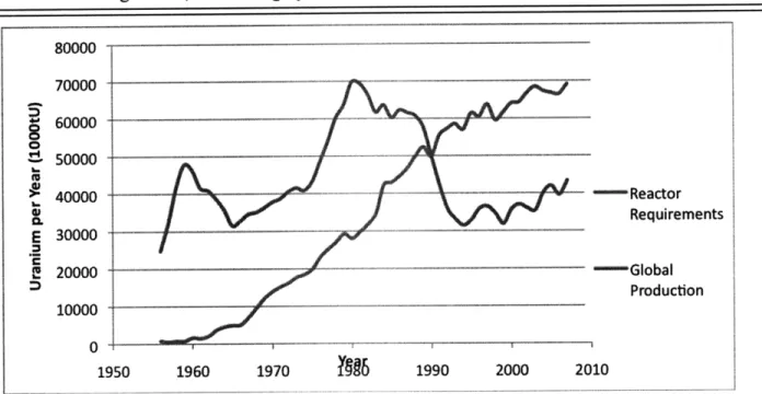
In order to model uranium peak production by the EIA model, an appropriate growth rate for pre-peak production must be estimated. Since the 1950's, annual uranium requirements for the world's nuclear reactors have grown fairly consistently year-over-year. Despite changes in regulatory regimes and boom-bust construction at the country level, global nuclear capacity has increased with time. Although reactor capacity additions have followed a mostly-monotonic trend, production has varied significantly over the same time frame. This trend, which is

illustrated in Figure 4.1, can be largely attributed to demand for uranium for cold war 80000 70000 60000 -50000 ' 40000 - - Reactor Requirements E 30000 1!20000 - --- Global 1Production 10000 1950 1960 1970 l 1990 2000 2010

Figure 4.1 Global Reactor Uranium Requirements and Annual Production since 1955. Production and reactor requirements are in 1,000 tU (OECD, 2008).

weapons programs. For the past 20 years, secondary supplies, primarily denatured HEU, have easily filled the gap between primary production and demand. Figure 4.1 shows that annual production patterns have not been monotonic. Consequently the future production growth rate

selected for this study was the average annual growth rate between 1993 and 2007, representing the post-cold war modem period. This growth rate of 1.5 % per year was used as a midline

estimate. An upper bound growth rate of 3.6 % per year was derived from the average growth in reactor needs from 1980 to 2007. On the assumption that within the next 5-10 years, secondary supply contribution will peak and remain level at -15,000 tU per year, the growth in primary production can be assumed to be equal to the growth in demand (IAEA 2006). A lower bound production growth rate of 0.5% per year was selected on the assumption that future nuclear growth may be below historical levels, and that the ability of producers to expand capacity may be lower in the future due to more difficult mining conditions.

To find a reasonable estimate for the Reserves/Production ratio to define post peak production habits, historical Canadian production data was consulted. In Table 4.1, the historical Table 4.1 Canada's Production, Known Conventional Resources (KCR), and KCR/Production

Year Annual Production RAR + EAR-I KCR/P Ratio

(1000 tU) (1000 tU) 1965 3418 847000 248 1967 3234 916300 283 1970 3520 586600 167 1973 3710 716000 193 1976 4850 585000 121 1977 5790 838000 145 1979 6820 963000 141 1982 8080 1018000 126 1983 7140 414000 58 1986 11720 411000 35 1988 12393 460000 37 1989 11323 439000 39 1991 8160 443000 54 1993 9155 471000 51 1995 10473 454000 43 1997 12031 430000 36 1999 8214 433000 53 2001 12522 436990 35 2003 10455 438500 42 2005 11628 443800 38 2007 9862 423200 43

production, known conventional resources (RAR + EAR-I), and KCR/P. Canada currently is the world's largest uranium producer. With a wealth of uranium resources, and government policies conducive to mining and exportation, Canada has served as a center of global uranium mining. Because the industry is well developed in Canada, and market economics govern the behavior of mining companies, the R/P ratios for Canada reflect efficient mining activity. Consequently an

R/P of 43.3 years, the Canadian average since 1983, was used to model future post-peak production behavior in the two-form model. The post-1983 period was chosen to reflect the stable, non-developmental stage of the Canadian industry.

The base assumption for total uranium supply was the 2007 Red Book estimate of RAR through SR, discounting the EAR-II and SR estimates by a factor of .85 to account for milling and mining losses. Remaining global supply was thus assumed to be 10,348,955 tU. A lower supply assumption, which accounted for 30 percent less EAR-II and 50 percent less SR, was also tested. Additionally a high supply scenario with 30 percent greater EAR-II and 50 percent

greater SR was tested.

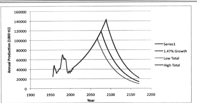
The result of the two form model for peak production using the three supply cases and an annual production growth rate of 1.5% is shown in Figure 4.2. The figure suggests peak

. . 160000 l ...

A

k/

\\\

Figure 4.2 Peak Uranium Production using the EIA Model with a production growth rate of 1.5 %.

production in 2067, 2076, and 2089 for the low, base, and high supply cases, respectively. Additionally, the peak production for different production growth rates was analyzed. Figure 4.3

-Seriesl

- 1.47% Growth

-0.5% Growth

- 3.57% Growth

1900 1950 2000 2050 2100 2150 2200

Figure 4.3 Peak Uranium Production using the EIA Model with the middle supply assumption and various production growth rates

140000 120000 100000 -80000 60000 40000 20000 0 1900

!!

.

.

.

.

...

.

...

...

.

'/

T---~

\\

_\

shows that peak uranium production occurs in 2045, 2076, and 2124 for production growth of 0.5%, 1.47 % and 3.57 %, respectively.

Next a per capita requirements model was applied to estimate future uranium needs assuming population growth and global development. From 1980 to 2000, an average of .055 kg of uranium was consumed per person per year in the United States. For the purposes of this study, the United States is taken to represent a developed nation with a midlevel dependence on nuclear power, i.e., approximately 20 percent of total grid power. If it is assumed that in the future, the rest of the world develops to post-industrial standards with nuclear power as a

significant source of energy, then the global annual uranium demand per capita can be assumed to be 0.055 kg/yr. Obviously a significant development time would be required given that

Greenfield plants are projected to take 15-20 years to build. Nevertheless, if by 2050 there were 8.9 billion people globally as current estimates reflect, the annual needs would be 489,500 tU. Even on the assumption that total uranium resources are the -10 million tons estimated today, with global consumption at the estimated rates, the world's uranium supply would be depleted by 2070.

Discussion:

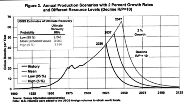
The results of this production peak study illustrate that a peaking scenario could occur by the middle of the 21st century. In Figure 4.2, the sensitivity of peak production to changes in the total global supply of conventional uranium was analyzed. In the EIA study of peak oil, Figure 4.4, which used similar analysis, the base case production peak occurred in 2037, with a low

Figure 2. Annual Production Scnarlos with 2 Pecent Growth Rats and Offerent Resource Leve (Decne RIP*10)

0

Figure 4.4 Peak Oil Production Scenarios for different total supply, and production growth estimates (Woods et. Al 2004)

supply estimate peak in 2026 and the high supply estimate peak in 2047. At a superficial level, the results of this study suggest that peak uranium is less of an imminent risk than peak oil. Nevertheless, deeper analysis reveals some important trends. First the sensitivity of peak projections to changes in the total supply was shown to be lower than the sensitivity to changes

in the production growth rate. In Figure 4.2, the three data sets representing the low and high supply estimates both result in supply peaks occurring within a range of 13 years of the base case. The changes in supply estimates, both approximately 20 percent of the total base

assumption, did not dramatically alter the peak date. This relative insensitivity can be interpreted to mean that specific fluctuations in Red Book supply estimates, which in recent years have been on the order of a couple of percent per year, are immaterial in determining the future supply situation.

Although the sensitivity of the peak date to total supply was small, the sensitivity to changes in the annual production growth rate was very significant. By limiting production

growth to 0.5% per year, uranium producers could extend peak production until 2124. On the other hand, if there were a fast run up in production to compensate for decreased availability of

secondary supplies, global stocks could peak within 40 years, and the long term viability of nuclear power could come into question. In the EIA study of the peak oil scenario, a high sensitivity to the production growth factor was also found. This parallel could be interpreted to mean that the long-term supply dynamics for crude and uranium are similar. On the other hand it may simply reflect that the two-form model is heavily dependent on the growth factor.

Nevertheless, this observation does suggest that developing a more accurate model for

production growth could be beneficial. More rigorous accounting for the physical structure of mines, the maximum drilling capacity per year, the equipment requirements for milling larger ore quantities, and the probability of flooding or other mining setbacks could yield a more reasonable growth model than the fixed rate assumption based on historical trends.

Another important factor in an accurate growth model is the producer's desire to produce at capacity. For-profit corporations are motivated to maximize shareholder equity. This can manifest itself in demonstrating earnings growth, which can be generated through greater

production. On the other hand, higher prices can also drive margins higher, and effectively boost earnings. If mining companies had pricing power, and collectively reduced production, this could create short-term supply pressures, which could drive prices higher. Another reason to reduce production would be to preserve the longevity of a given mine. This could be a function of a company's desire to have a sustainable business model and not to exhaust its resources too quickly. It could also simply be a reflection of the speculative view that uranium prices will be higher in the long-run.

The post peak KCR/P ratios for uranium are significantly larger than the R/P ratios for oil. Superficially this appears to be a noteworthy distinction between the oil and uranium markets; however, much of this different may be attributed to the different taxonomies use in both resource markets. In the uranium markets, known conventional reserves (KCR) represents the sum of RAR and EAR-I. With oil R/P ratios, there is some ambiguity as reserves could technically refer to iP, 2P, 3P, or 4P reserves; however, by convention oil's R/P is calculated by

dividing proved reserves (1P) by that year's production. Consequently the large difference between these ratios may be due to the fact that KCR uranium and IP oil are not perfectly

analogous'. If these ratios were considered to be equivalent, then they could be interpreted to show a fundamental difference in the way uranium and crude producers operate. An R/P of 10 reflects an aggressive approach to production, with a larger emphasis on maximization of output as opposed to sustainability. Uranium's higher KCR/P of 40 can be interpreted in a few different ways. First, it could show that uranium is a less competitive industry. The availability of

secondary supplies and a relative lack of market participants may have caused producers to only produce under the most lucrative of environments without a fear of losing share. Another

possibility is that uranium miners are less short-sighted than oil producers, and want their resources to sustain the nuclear power indefinitely. Finally, the high R/P could show that the technology and mining processes are less refined for uranium, and higher production simply isn't possible. The flooding at Cameco's Cigar Lake facility would seem to support this argument, as mining risks can unexpectedly and dramatically reduce companies' outputs.

1 It is not possible to perfectly reconcile the taxonomies for oil and uranium; however, if RAR were used for reserves instead of KCR in the ratio calculation for uranium, the average RAR/P from 1983 to 2007 would have been 29.1 years, still significantly higher than that of oil.

The fixed stock-per capita proved to be somewhat less useful in analyzing the uranium market than the copper markets. The main distinction is that although some copper goes to waste, it is a commodity that is recycled and remains in use in infrastructure, homes, electronics, etc. On the other hand uranium can be seen as somewhat of a combustible, in that in the absence of reprocessing, once it is used as fuel, it cannot be reused. Although the analysis of annual needs was not exactly analogous to Graedel's fixed-stock-in-use, it was revealing of the potential impact of population growth and global development on the lifetime of the world's uranium supply. Although the availability of construction materials, proliferation concerns, 'nimby' politics, and unrealistic modernization expectations would all stand in the path of massive scale nuclear development by 2050, the notion of the current supply being sufficient to sustain only 20 years of power is somewhat frightening. One takeaway from this observation is that the fuel needs of each newly constructed plant should be accounted for so that there is some sense for how annual global needs are evolving.

5. Development of a Model for Exploration Expenditure

To develop a model for exploration expenditure, empirical values for discovery time, development time, and production lifetime of uranium mines were needed. From the Red Book retrospective, these could be extracted from the timelines for the world's largest uranium mines that have closed. Table 5.1 shows these times where available, and calculates the average value Table 5.1 Discovery time, development time, and production lifetime for the world's largest uranium mines

Mine Exploration to Discovery to Production

Discovery Time Production Time Lifetime

(Years) (years) (years)

Beverley 2 30 Honeymoon 4 Jabiluka 3 Olympic Dam 6 12 Ranger 1 12 Lagoa Real 7 19 Cigar Lake 12 Cluff Lake 15 5 22 Key Lake 7 8 16 8 13 Macarthur River 7 11 McClean Lake 5 20 Rabbit Lake 3 7 Jachymov 18 Prbram 41 Rozna 0 3 48 Straz 0 2 29 Bellezanne 20 9 17 Ecarpiere 2 5 33 Dabat 3 4 39 La Commanderie 4 1 35 Le bernardan 9 13 24 Le Chardon 7 0 34 Margnac 3 5 41 Mas D'Alary 1 20 7 Mas Lavayre 7 14 19

Moumana 1 5 14 Oklo 13 2 29 Culmitzsch 0 3 14 Freital 0 22 21 Lichtenberg 10 0 19 Paitzdorf 2 0 40 Schmirchau-Reust 2 0 40 Mecsak 2 2 41 Inkay 3 22 Kanzhugan 2 14 Melovoye 3 34 Moynkum 25 Mynkuduk 2 12 Uvanas 6 8 Zaozernoye 6 Rossing 7 3 14 Langer-Heinricj 3 33 Abkorum 23 Akouta 16 6 Arlit 9 6 Ebba 26 Imouraren 21 Techili 32 Avram lancu/Bihor 4 8 37 Antei 35 Dalmatovskoye 0 Luchistoye 6 Martovskoye 0 10 21 Oktyabrskoye 0 7 Streltsovskoye 6 Tulukuevskoye 3 Michurnskoye 3 4 Severinskoye 10 Crow Butte 2 11 Lucky Mc 1 34 Shirley Basin 2 33 Smith Ranch 1 10 1 Jackpile-Paguate 2 2 29 Highland 1 5 10 Mt. Taylor 2 16 3 Average 6.31 9.13 25.97

for each time period. The average discovery time, development time, and production lifetime, were found to be 6.31 years 9.13 years, and 25.97 years, respectively. Although Table 5.1 shows that the development times vary widely from mine to mine, the timeframes for discovery and production lifetime were fairly consistent across the data. Nevertheless, there was significant variability in the development times for mines that began production during different periods, and consequently, development time was averaged over three separate periods. For the periods prior to 1975, 1975-1995, and 1995-2008, the average development times were 3.91 years, 11.06 years, and 24.38 years, respectively. These values were used in the NPV calculations.

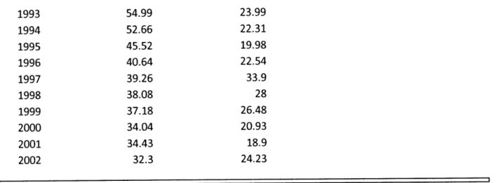
Next, the market prices for uranium were considered over time. The NUEXCO spot price for uranium was used as the benchmark spot price for uranium. Approximately 65% of uranium is sold through long-term contracts with specific structures such as caps, floors, and escalators. To relate long-term uranium to spot prices, EURATOM data from 1980 to 2002 was considered. Over this time period, spot and multiyear contract prices varied significantly as shown in Table 5.2. Over this time period, multi-annual contracts prices had a premium of 77 percent

Table 5.2 EURATOM Spot and Multi-year Contract Uranium Prices from 1980-2002

Year EURATOM Multi-Annual EURATOM Spot

($/kg) ($/kg) 1980 93.4 90.82 1981 86.74 73.05 1982 83.16 62.38 1983 80.55 60.42 1984 77.42 50.09 1985 75.42 38.83 1986 80.25 45.95 1987 84.53 44.85 1988 82.6 41.89 1989 76.18 31.63 1990 76.2 25.08 1991 67.89 23.56 1992 64.35 25.03 36

1993 54.99 23.99 1994 52.66 22.31 1995 45.52 19.98 1996 40.64 22.54 1997 39.26 33.9 1998 38.08 28 1999 37.18 26.48 2000 34.04 20.93 2001 34.43 18.9 2002 32.3 24.23

relative to the average spot price from the previous 3 years. Using this premium as a factor, long-term price of uranium (Pt) for a given period of time was calculated according to the Equation 3.2. The aggregate prices of uranium since 1972 were calculated and are shown in Table 5.3. These aggregate prices were used in the calculation of the NPV of exploration.

Table 5.3 NUEXCO Spot and Calculated Aggregate Uranium Prices since 1972

Year NUEXCO Spot Aggregate Price

($/kg) ($/kg) 1972 15.21 23.42 1973 16.67 24.10 1974 28.88 33.41 1975 61.62 62.67 1976 103.22 110.42 1977 109.72 143.70 1978 112.37 164.09 1979 110.66 166.34 1980 82.68 146.18 1981 62.89 120.28 1982 51.74 93.78 1983 59.75 87.79 1984 44.9 75.69 1985 40.58 69.90 1986 44.2 65.20 1987 43.6 64.49 1988 37.83 61.42 1989 26 50.30 1990 25.38 43.10

1991 22.6 36.28 1992 20.7 33.58 1993 18.24 29.98 1994 18.33 28.38 1995 21.97 30.14 1996 33.49 40.02 1997 27.39 41.36 1998 23.61 40.67 1999 21.45 35.29 2000 18.04 30.51 2001 21.06 30.59 2002 25.69 33.84 2003 25.41 36.57 2004 40.81 49.53 2005 62.744 71.42 2006 108.394 119.22 2007 218.526 225.92 2008 135.762 224.96

Another component of the NPV calculations for exploration investment is the availability of credit. Uranium miners typically finance their exploration through a variety of methods. Typically bank lines of credit are tapped or equity private placements are made; however, some regulatory environments allow for different financing options. For example, in Canada there is a tax provision which allows exploration companies to issue flow-through shares, which are common equity shares that pass tax credits onto investors which can be applied to their personal or corporate income tax. This tax benefit makes the shares more valuable to investors, allowing miners cheaper financing at no expense. Due to the diversity of financing options, calculation of an appropriate discount rate by the CAPM model could prove very difficult. Consequently, long-term bond yields of uranium producers were used to estimate the availability of financing and the risks of exploration investment. Although junior uranium miners are unable to issue debt, and thus don't have associated credit spreads, the large uranium producers were used as a

benchmark. In 1995, Cameco issued 10-year bonds with AAA rating, while their short term 38

debentures issued in 2001 carried a credit rating of A. Most recently, Cameco debentures have carried a BBB+ rating. Between 1991 and 1996, BHP Billiton issued long-term debt which was

all rated between A- and A+. As of 2008, Rio Tinto's long-term credit rating was BBB+. On the assumption that most uranium companies are weaker credits than the majors, the historical yields for BBB paper were used as the benchmark discount rate in this model. The yields of BBB and AAA-rated paper as well as the United States 10-year treasury notes are shown in Figure 5.1.

I ---- I_._~.--

4--AAA Yield

BBB Yield

-U.S. 10-Year Yield

1960 1970 1980 1990 2000 2010

Figure 5.1 Yields for AAA and BBB bonds and United States 10-year Treasury Notes from 1970 to 2008 (WRDS, 2009)

The data in figure show that the average credit spread for BBB bonds has been 98.6 basis points. Finally, an assumption needed to be made on the costs of production. These include corporate overhead, mine development costs, reagent costs, licensing costs, labor costs, as well

as environmental costs. These costs have increased over time most directly as a function of increased regulation and growing demand for surveying and drilling equipment (Roberts). Conversations with uranium industry practitioners revealed that when the uranium price drops below 40 $/lb, companies begin cutting production due to it not being economical (Roberts).

18 S16 C 1 14 12 10 8 6 c 4 C 2

Consequently, production costs were modeled as a linear function increasing from 25 $/kgU in 1970 to 85 $/kgU in 2007. In addition, it was assumed that 75 percent of a mine's total reserves were produced evenly over the first half of the production lifetime, with the remainder evenly produced over the final half.

Given these assumptions the NPV of investing $ 1,000,000 in exploration in a given period was calculated according to Equation 3.3. The NPV of exploration for a given period was plotted against the actual investment in Figure 5.2. Because the trend appeared fairly linear,

6000.00 y = 0.007x -3E+06 SR 2 = 0.704 S 4000.00 "- - __... .-- E * NPVof MM 2000.000 -.---- ---- . ..

M

-6

0 00_0 0 ...

...

. . . ...

. ...

Figure 5.2 The relationship between calculated NPV and actual uranium exploration investment from 1970 to 2007.

a linear regression was performed to relate NPV to actual exploration investment. The resulting linear equation,

where I is total annual exploration investment in $/year and NPV is in $. This line had a regression coefficient of 0.836. Finally this model was used to calculate investment using the

market conditions from 1970 to 2007, and was plotted against the actual values in Figure 5.3.

1400000000.00 1200000000.00 1000000000.00 00000000.00 600000000.00 - Actual Exploration 400000000.00 Investment 200000000.00 - - Calculated Exploration Investment 0.00 19 5 1970 1975 1980 1985 1990 1995 2000 2005 2010 -200000000.00

Figure 5.3 Comparison of Model Predicted Exploration Investment Versus Historical Exploration Investment from 1970 to 2007.

Although the model does not perfectly trace the historical investment, it does follow a similar form to the historical trends.

Discussion:

The development of this model for uranium exploration investment revealed that a multitude of variables go into a mining company's decision to invest in exploration. Although the market price for uranium is certainly a large factor in the potential upside for investment, the

significant economic risk associated with discovery and then the significant time delay between discovery and production make the investment prospect far less appealing than might be thought on the basis of high spot uranium prices.

It is important to note that in Figure 5.3, the model that was developed is back tested on the data from which it was derived. By back testing on this data, it is expected that the calculated values should be similar to the historical values. Although Figure 5.3 illustrates how well model performed over historical conditions, it is clearly not a perfect fit. Each of the assumptions made

in deriving the model impacted the final result, so it is necessary to evaluate each of those error sources. The values used for discovery, development, and production lifetimes were all based on historical averages. These historical averages were for the largest uranium mines, but did not

account for smaller developments for which data is not readily available. It is possible that a more comprehensive data set could have provided more reasonable estimates for each of those

characteristic times. In the case of development time, the average time was taken for three distinct periods because a trend of increasing development time was observed. Although there was no obvious trend in production life and discovery time, subdividing into averages over different time periods could have provided more appropriate timing estimates for the model.

In addition to error in the timing assumptions, the development of an accurate price proved to be difficult. Uranium futures do trade on the NYMEX along with crude oil and other major commodities; however, uranium insiders all agree that futures are not a reflection of long term prices in the uranium markets. Because the contracts used by miners are private, and no standard formula exists, an aggregate price that accounts for the relationship between long-term and spot prices had to be developed. As evidenced by the fact that the historical EURATOM spot prices were historically higher than the NUEXCO settling spot prices (which are taken as the global standard), the relationship between EURATOM spot and multi-year prices is unique to that market. Discussion with traders from different mining companies would likely reveal a more useful method for estimating long term prices. Another potential flaw is the assumption that

companies would use current long-term contract prices as an assumption for the prices far off in the future when production begins. Currently the average time from exploration to production is on the order of 30 years, so the prices used to sell the next five years of production could be orders of magnitude different from those in 30 years. It may be best to include a long term scaling factor in the aggregate price that reflects a mining company's view on uranium prices 10's of years into the future.

The availability of credit is arguably the most significant factor in all business decision making. Without access to capital, projects simply cannot go forward. While this qualitative fact is well understood, this force held significant weight in the calculation ofNPV. Credit, as manifest in the discount rate, has an exponential impact in this model due to the compounding over multiple years. Because a significant portion of financing for mining is done through equity raises, is difficult to say whether or not BBB bond yields reflect appropriate financing rates for miners. Nevertheless, Figure 5.1 shows that over time, the yields for AAA and BBB bonds have traded at a fairly fixed spread to long-term treasuries. That said, BBB bonds do reflect the general rate markets which is historically the primary driver of credit availability.

The discovery costs that were used for these calculations basically divided the total exploration expense by the total discovered (RAR +EAR-I) and produced uranium. Embedded in this discovery cost is a probability of discovery. Because mining insiders explain that the low hanging fruit is the first to get picked off, and that the ore quality in newer discoveries is lower than in the earliest studies, there must be time variation in the discovery costs. Nevertheless, without any way to see the time variation for this factor, a historical average had to be used. In estimating production costs, a linear ramp with time was used to reflect increasing equipment costs and overhead, increased difficulty in mining (lower ore quality), and increased

regulatory and surveying costs. While the current value for production costs was based on discussion with a member of the mining industry, the assumption of a linear slope may be inaccurate. It is possible that a stair-step function would have been better than a linear model, because production costs may remain level on a period to period basis. Use of the purchasing power index (PPI) or the consumer price index (CPI) may have better reflected the costs of producing uranium since 1970.

One aspect of the results that proved surprising was that negative NPV values were found for investment during many of the historical periods. Because the discovery cost has an

embedded probability, a negative NPV means that investment is expected to have a negative return for a given period. With mining companies operating rationally to grow profits, a negative NPV should imply that no money should be invested in exploration in a given year. As

mentioned earlier, each of the assumptions used in the model has limitations and is a potential error source, so getting any or many of these factors wrong may have caused NPV's to incorrectly be negative.

Another explanation lies in the fact that the NPVs calculated are averages for the entire industry. Within that industry, one can only expect that there are miners with low discovery and production costs; access to cheaper financing than their peers; better pricing power with their contracts, and better government ties to shorten development times. For these producers,

exploration may very well be highly economical in years when the average NPV is negative, and subsequently the existence of exploration investment is very easily explained.

Analysis of the relationship between NPV and actual historical expenditure revealed a fairly linear trend which was ultimately used to complete this model. The R value, 0.836, for the linear regression of that data revealed that a linear model did a reasonably good job of describing