Exploration of the relationship between water main breaks and temperature covariates

Publisher’s version / Version de l'éditeur:

Urban Water Journal, 9, 2, pp. 67-84, 2012-05-01

READ THESE TERMS AND CONDITIONS CAREFULLY BEFORE USING THIS WEBSITE.

https://nrc-publications.canada.ca/eng/copyright

Vous avez des questions? Nous pouvons vous aider. Pour communiquer directement avec un auteur, consultez la

première page de la revue dans laquelle son article a été publié afin de trouver ses coordonnées. Si vous n’arrivez pas à les repérer, communiquez avec nous à PublicationsArchive-ArchivesPublications@nrc-cnrc.gc.ca.

Questions? Contact the NRC Publications Archive team at

PublicationsArchive-ArchivesPublications@nrc-cnrc.gc.ca. If you wish to email the authors directly, please see the first page of the publication for their contact information.

NRC Publications Archive

Archives des publications du CNRC

This publication could be one of several versions: author’s original, accepted manuscript or the publisher’s version. / La version de cette publication peut être l’une des suivantes : la version prépublication de l’auteur, la version acceptée du manuscrit ou la version de l’éditeur.

For the publisher’s version, please access the DOI link below./ Pour consulter la version de l’éditeur, utilisez le lien DOI ci-dessous.

https://doi.org/10.1080/1573062X.2011.630093

Access and use of this website and the material on it are subject to the Terms and Conditions set forth at Exploration of the relationship between water main breaks and temperature covariates

Rajani, B. B.; Kleiner, Y.; Sink, J-E.

https://publications-cnrc.canada.ca/fra/droits

L’accès à ce site Web et l’utilisation de son contenu sont assujettis aux conditions présentées dans le site LISEZ CES CONDITIONS ATTENTIVEMENT AVANT D’UTILISER CE SITE WEB.

NRC Publications Record / Notice d'Archives des publications de CNRC:

https://nrc-publications.canada.ca/eng/view/object/?id=7c91a647-aadd-40db-9701-39533b682647 https://publications-cnrc.canada.ca/fra/voir/objet/?id=7c91a647-aadd-40db-9701-39533b682647

Exploration of the relationship

between water main breaks and

temperature covariates

Rajani, B.B.; Kleiner, Y.; Sink, J-E.

NRCC-54537

A version of this document is published in :Urban Water Journal, 9, (2), pp. 67-84, 2012-05-01, DOI:

10.1080/1573062X.2011.630093

The material in this document is covered by the provisions of the Copyright Act, by Canadian laws, policies, regulations and international agreements. Such provisions serve to identify the information source and, in specific instances, to prohibit reproduction of materials without

written permission. For more information visit http://laws.justice.gc.ca/en/showtdm/cs/C-42

Les renseignements dans ce document sont protégés par la Loi sur le droit d’auteur, par les lois, les politiques et les règlements du Canada et des accords internationaux. Ces dispositions permettent d’identifier la source de l’information et, dans certains cas, d’interdire la

Exploration of the Relationship between Water Main Breaks and

Temperature Covariates

Balvant Rajani, Yehuda Kleiner, and Jean-Eric Sink National Research Council Canada

ABSTRACT: Water utilities (especially in colder climates) often experience an increase in water main breaks in colder seasons. Some observers argue that this increase largely occurs during the period when there are sudden and prolonged changes in water and air temperatures, which typically occur during the late fall to early winter (temperature drop) and late winter to early spring periods (temperature rise).

This paper examines the impact of temperature changes on observed pipe breakage rate for three pipe materials, namely, cast iron, ductile iron and galvanized steel. Several water and air temperature-based covariates were tested in conjunction with a non-homogeneous Poisson pipe break model to assess their impact on water main breaks, using data sets from three different water utilities in the USA and Canada. Temperature-based covariates, such as average mean air temperature, maximum air temperature increase and decrease, and how fast the air temperature increase and decrease over a specific period of days, were found to be consistently significant. While the availability of water temperature data (which most utilities do not have) can enhanced the prediction of water main breaks, it appears that air temperature data alone (which most utilities can access) are usually sufficient.

Keywords: Water and air temperature-based covariates, impact of temperature on water main breaks, non-homogeneous Poisson probabilistic model.

Introduction

Water utilities (especially in colder climates) often observe a peak in main break frequency during periods when the air temperatures approach 0oC. Some observers also assert that the increase in breakage frequency occurs when the air temperature transits from above 0oC to below 0oC or vice versa, e.g., during late fall (drop) and early spring (rise). Others argue that water temperature has a higher impact on pipe breakage rates; hence it, rather than air temperature, is the appropriate variable to correlate with the breakage frequency. Others yet postulate that the temperature difference between the water in the pipe and the surrounding soil/backfill

contributes to elevated breakage rates. However, the reality is that water or ground temperature data are rarely available to evaluate their impact on breakage frequency.

Both water and air temperature data were measured in a recent study reported on by Hughes et al. (2010) in Connellsville, Pennsylvania. Data from this study and two other Canadian water utilities (from which only air temperature data were available) are used in this paper to ascertain the impact of temperature on main breaks. Several air and water temperature-based covariates are constructed to reflect how temperature and temperature fluctuations may impact observed breakage rates for three pipe materials, namely, cast iron, ductile iron and galvanized steel. These temperature-based covariates are used in conjunction with a probabilistic pipe break prediction model to identify which of them make significant contributions to explain the observed main breaks.

The remainder of this paper is organized as follows. In the next section, previous studies on temperature-based covariates and how these correlate with main breaks are examined and discussed. The third section briefly describes the available data from the three utilities and takes a preliminary look at key data to see if breaks and commonly used temperature-based covariates have any obvious correlation. The fourth section describes the probabilistic model used to identify the most promising temperature-based covariates. The fifth section applies the

probabilistic model to the data from the three utilities. Summary and conclusions are provided in the final section.

Review of past studies

The effects of temperature on pipe breakage rates have been observed and reported by many. Walski and Pelliccia (1982) suggested that pipe breakage rates might be correlated to the

maximum frost penetration in a given year. They used the air temperature of the coldest month as a surrogate for unavailable frost penetration data. They used a multiple regression model with pipe age and air temperature as covariates,

BT At e e t N T t N( , )= ( ₀) (1)

where t = pipe age; N(t0) = breaks per pipe length at year of installation; T = average air

information as to the quality of breakage predictions that they obtained using this model. The analysis was conducted on an annual basis, i.e., time step or time period was one year.

Newport (1981) analyzed circumferential pipe breakage data from various areas of the Severn-Trent Water Authority in the United Kingdom. He found that increased breakage rates coincided with cumulative degrees-frost (usually referred to as freezing index in North America and expressed as degree-days) in winter as well as with very dry weather in the summer. He attributed the increase in winter breakage rates to the increase in earth loads due to frost penetration, i.e., frost loads, and the elevated summer breakage rates to the increase in shear stress exerted on the pipe by soil shrinkage in a dry summer. He also observed that when two consecutive cold periods occurred, the breakage rates (in terms of breaks per degree-frost) in the first one exceeded those of the second one. He rationalized that the early frost “purged” the system of its weakest pipes, causing the later frost to encounter a more robust system. Newport (1981) used data of 7 years (1970-1977) to obtain a linear relationship (correlation coefficient of 0.9) between the number of water main breaks and the cumulative degrees-frost in a given year

Total breaks per year = 2.5(Total degrees of frost) + 500 (2)

The above relationship was derived for the Soar division of the Severn Trent distribution system and the total length of water mains was not specified. This linear model suggests that every degree of frost is responsible for an additional 2.5 breaks. No model was given to predict water main breaks during extreme dry weather. The analysis was conducted using a time step or time period of one year.

Bahmanyar and Edil (1983) investigated the relation between air temperature and mains breaks in Madison, Wisconsin. They observed that number of breaks increased markedly when the temperature dropped suddenly and this drop was sustained for several days (cold snap). Their field and laboratory studies also confirmed that longitudinal strains that lead to circumferential breaks in small diameter mains increased when the rate of freezing is rapid, i.e., temperature drop occurs over a small number of days.

Habibian (1994) analyzed the distribution system of Washington Suburban Sanitary Commission, Maryland, and observed an increase in water main breakage rate as the

rather than to the ambient air temperature, reasoning that although their monthly averages are similar, ambient air temperatures display sharp fluctuations while water temperatures are better surrogates for underground pipe environment. He concluded that the water temperature drop, rather than the absolute water temperature, had a determining influence on the pipe breakage rate. He also observed that in a given winter, similar consecutive temperature drops did not necessarily result in similar breakage rates, however, typically a surge in the number of pipe breaks occurred every time the temperature reached a new low. His explanation for this

phenomenon concurred with Newport (1981), namely, that every temperature low “purged” the system of its weakest pipes, thus a new low affected the pipes that were a little more robust than those that had broken in the previous cold spell. The pipes continue to deteriorate during the warm seasons and the process is repeated in subsequent cold seasons. It should be noted that Habibian’s (1994) observations were all based on one-year data and that the time of the breaks was based upon when water from the broken pipes surfaced.

Lochbaum (1993) reported on a study conducted by Public Service Electric and Gas Company, which showed that the breakage rates of cast iron gas pipes increased exponentially with the number of degree-days (degree-days were defined as Σ_i⊂N [(65oF-Ti], where Ti is the

average temperature in oF in day i and N is the set of days in a given month with average

temperature below 65oF). Lochbaum (1993) did not present a model relating the number of water main breaks to monthly degree-days; her observations, however, agreed with those of Newport (1981) and others. No information was provided as to the causes of pipe breaks in warm seasons.

Sacluti et al. (1999) applied an artificial neural network (ANN) to the distribution system of a sub-division in Edmonton, Canada. The ANN model was applied to the small network as a single entity (rather than to individual pipes) and was trained on data that included temperature (water and ambient), rainfall, operating pressure and historical data on the number of breaks. The network consisted of spun-cast 150-mm (6”) water mains. A sensitivity analysis determined that rainfall and operating pressure did not contribute to the predictive power of the model, and these were therefore omitted. The model predicted the number of water main breaks based on a 7-day (time step of 7 days) weather forecast. The authors claimed that the model was successfully

applied to a holdout sample, demonstrating that the ANN “learned” the breakage patterns rather than memorized them2.

Ahn et al. (2005) explored the use of ANN to relate breaks to water and soil temperatures. They observed that the number of main breaks increased when the water and soil temperatures changed in the spring and in the fall. Although, Ahn et al. (2005) indicate that their model was able to predict the number of breaks, there is insufficient detailed information to assess if the data they present explained the influence of water or soil temperatures on main breaks. Again the analyses were conducted on data collected over a one year period.

Goodchild et al. (2009) also examined several climatic covariates to see if they could explain the timing of observed water main breaks. They explored covariates such as daily minimum grass temperature, minimum temperature, rainfall, solar radiation, run of wind,

evapotranspiration, actual evaporation, water content in the topsoil, and soil moisture deficit. They proposed a multi-covariate linear relationship to predict the number of water main breaks as function of these covariates. They applied the model to main breaks data collected over six years in two regions in the United Kingdom and they identified actual evaporation, daily rainfall, minimum grass temperature, and soil moisture deficit to be significant covariates for predicting breaks observed in cast iron and asbestos cement pipes buried in loam and clay. They could not establish similar relationships for cast iron (CI) pipes installed in sand and silt and for other pipe materials such as ductile iron, steel, PVC and PE. It is important to note that they did not validate their model using a holdout sample.

Kleiner and Rajani (2004, 2009) considered 3 climate covariates in predicting annual water main breaks, namely, annual freezing index (FI), cumulative annual rain deficit (RDc) and snapshot rain deficit (RDs). FI is a surrogate for the severity of a winter in a given year, RDc is a surrogate for average annual soil moisture and RDs is a surrogate for locked-in winter soil moisture (appropriate for cold regions, where soil can freeze in the winter). These covariates were used in a deterministic model as well as in a probabilistic model to predict annual expected breaks for a homogeneous group of pipes. The analyses using these models were conducted

2

In ANN there is always a concern that the model will be “over-trained” resulting in a model that is just capable of “memorizing” the training data set rather than being able to generalize the patterns to new sets.

using a time step or time period of one year. It is important to note that with the exception of Sacluti (1999), all other models use a period of one-year for analysis.

Initial examination of break and temperature data

Water main break data from the three water utilities (Connellsville, Ottawa and Scarborough) were examined to see if rudimentary temperature-based covariates (such as mean temperatures) had an obvious impact on water main breaks. Seven homogeneous pipe groups (with respect to vintage, pipe diameter and pipe material) were formed from the data provided by the three water utilities as described below and summarized in Table 1. The analyses were performed on these selected homogeneous groups to account for the possibility that temperature-related factors may impact each pipe group differently. Since pipe length information was not available for data from Connellsville, all the analyses were conducted on absolute number of breaks rather than breaks per unit length of pipe.

Connellsville (Pennsylvania) data

Most of the water mains in the distribution network in Connellsville are cast iron and galvanized steel with some ductile iron, asbestos cement and PVC pipes. Nearly 80% of the 90 km (57 miles) of mains are over 100 years old. Data on a total of 339 main breaks were available for the period between January 2003 and December 2008. More details on the water distribution network in Connellsville can be found in Hughes et al. (2010). Two homogeneous groups of pipes were established from the Connellsville data, namely, CV-3 (cast iron) and CV-4 (galvanized steel). Predominant failure types on galvanized steel pipes were corrosion holes and longitudinal splits, while cast iron pipes had circular breaks, corrosion holes and longitudinal splits. Cast iron pipes are of 2½”, 4”, 6” and 8” diameter while, galvanized pipes were of 2” diameter. It appears that galvanized steel was a pipe material of choice for small diameter applications in the period 1880 to 1900. Mains are typically buried at a depth of 1.2 m (4 ft).

Air and water temperatures were monitored over a 3-year period (June 2005 to December 2008). Water temperature was measured once a day, immediately downstream of the treatment plant (which is close to the city). This daily temperature value was assumed in the analysis to represent the mean daily water temperature in the distribution network. The mean daily air temperature was measured at the treatment plant.

Ottawa (Ontario) data

The Ottawa pipe inventory included 16,383 individual pipe records (2,200 km total length) each with material type, diameter, installation year and the year retrofit cathodic protection (CP) was applied. For simplicity, cathodic protected pipes were excluded from the analysis. Soil data and service connection data were not available for each pipe. Break history data included the year and month of each breakage (repair) event from 1972 to 2001, as well as the type of break. One pipe group, Group OT-1 was established for analysis from the Ottawa data, consisting of cement-lined spun cast iron (CI) pipes, 150 mm (6”) in diameter, installed between 1954 and 1974. The availability of break type data enabled to select for Group OT-1 pipes that had experienced only circular breaks, longitudinal splits or corrosion holes, which were assumed to be the only break types that might be affected by temperature. The total length of the water mains in Group OT-1 was 230 km and the total number of breaks recorded was 1,033. Only break data from 1972 to 1989 were considered for pipes in Group OT-1 because Ottawa embarked on a hot spot cathodic protection (HS CP) program in 1990 that likely imposed a substantial change in breakage pattern. Water mains in Ottawa are typically installed at a depth of 2.4 m (8 ft) and mean daily air temperature data were obtained from Environment Canada.

Scarborough (Ontario) data

The Scarborough pipe inventory included 6,879 individual pipe records (a total of 1,155 km), each with material type, diameter, installation year and the year retrofit CP was applied. Nearly all the pipes had been installed in silty clays and therefore soil type could not be used as a pipe grouping criterion. Break history data included year and month of each breakage (repair) event from 1962 to 2003, as well as the type of break. Four homogeneous pipes groups (SC-1, SC-2, SC-3 and SC-4) were established for analysis from the Scarborough data. These pipe groups comprised 150 mm diameter pipes that experienced only circular breaks, longitudinal splits, and corrosion holes. Consequently, groups were largely established on pipe material and vintage and excluded pipes that had cathodic protection (hot spot began in 1984 and retrofitting began in 1986) for the same reason as articulated for the Ottawa data. Group SC-1 consisted of pipes installed between 1921 and 1935, which corresponded to the period when largely pit cast iron mains were produced. Group SC-2 consisted of pipes installed between 1943 and 1955, which corresponded to the period when small diameter spun cast iron mains were largely used. Group SC-3 consisted of spun cast iron pipes installed between 1956 and 1978. The vintage of OT-1 is

comparable to that of SC-3. SC-4 consisted of ductile iron pipes installed between 1960 and 1983. It should be noted that the majority of breaks in cast iron pipe groups (OT-1, SC-1, SC-2 and SC-3) are of the circular type while most of breaks in ductile iron pipe group (SC-4) are a result of corrosion holes. This observation concurs with the fact that ductile iron pipes (without manufacturing defects) largely fail by perforation and do not experience physical fracture, which is more typical of brittle materials like cast iron pipes. Thus, the use of the term “break” for a ductile iron pipe is a misnomer and the term “repair event” may be more appropriate. Water mains are typically installed at a burial depth of 1.5 m (5 ft) in Scarborough. As for Ottawa, mean daily air temperature data for Scarborough were obtained from Environment Canada.

Influence of mean air and water temperatures and of time step size

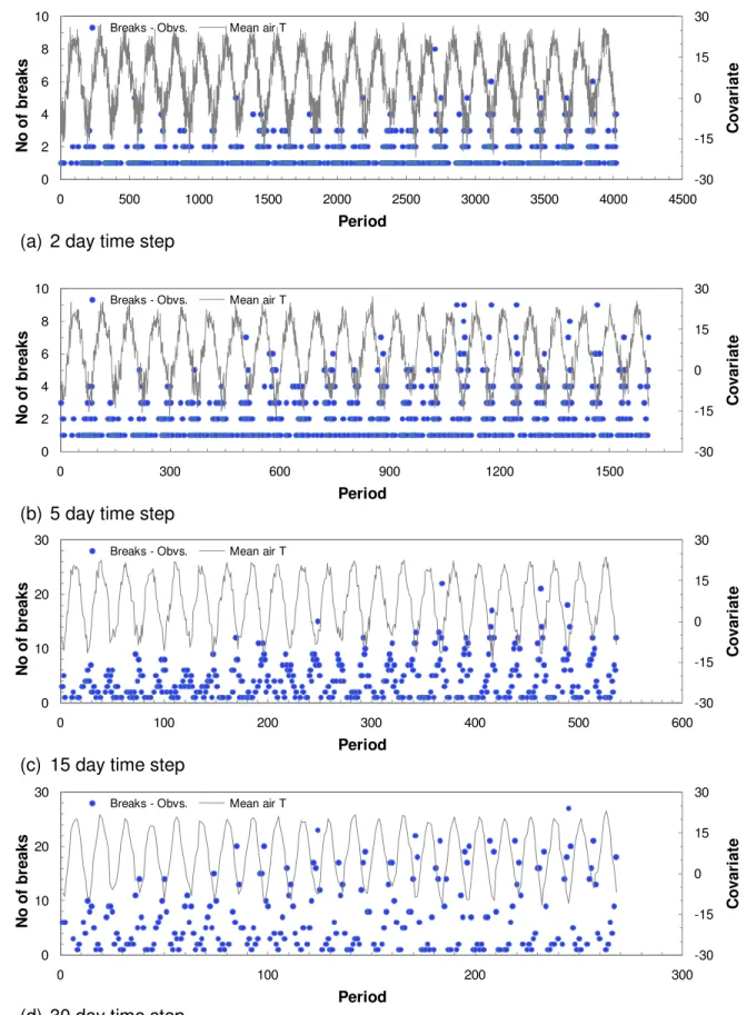
As a preliminary examination, mean air (and water for CV-3 and CV-4 only) temperatures and main breaks were plotted against time for the seven groups. Various time step sizes (duration) were used, over which mean temperatures were computed and number of breaks counted. Data for Connellsville were available for a relatively short period of 3½ years as compared to Ottawa and Scarborough where data were available for 18 and 22 years,

respectively. Fig. 1 provides a typical temperature and main break time histories for time steps of 2, 5, 15, and 30 days for the (CV-4) pipe group and Fig. 2 for the SC-2 group. For Connellsville, where both water and air temperature data are available, it can be clearly seen that both

temperatures move in sync with seasonal changes, although water temperatures are generally more restrained (smaller amplitude) than air temperatures, especially in the low range (water is not likely to freeze in the mains as they are typically buried below the frost line). Typically one or two breaks occur at most in a short time step, and more in longer time steps. The higher number of breaks for a longer time step makes it somewhat easier to visually correlate number of breaks with temperatures. However, even for time steps of 15 or 30 days, no clear and

unequivocal relationship is immediately apparent between the number of water main breaks and mean air and/or water temperatures. Consequently a probabilistic-based model was developed to determine, if any, relationships exist between water main breaks and various temperature-based covariates and if such relationships are dependent on the analysis time step size.

Proposed non-homogeneous Poisson model

The non-homogeneous Poisson (NHP) model has been extensively used by researchers to represent the probability of observing a number of breaks on water mains (e.g., Constantine and

Darroch, 1993; Constantine et al., 1996; Miller, 1993; Røstum, 2000; Economou et al., 2008; Kleiner and Rajani, 2009). The non-homogeneous Poisson model was used in this study to explore the relationship between water main breaks and water or air temperatures. A modified form of the Poisson model proposed by Kleiner and Rajani (2009)is used here, where the probability P(ki), of observing ki breaks in time step i, in terms of one or more time-dependent

covariates is, ! ) exp( ) ( i i k i i k k P i λ λ ⋅ − = where λ_i =exp[β_o +ψτ(g_i)+βq_i] (3)

where λ is the expected number of breaks (or the rate of occurrence of breaks) in time step i, _i β_o is a constant,

i

q is a row vector of time-dependent covariates prevailing at time step i and β is a column vector of the corresponding coefficients to covariates q. Time step i is taken relative to the first time step of reference,i_o, for which breakage records are available. The function

)] (

exp[ψτ g_i , whereg is the pipe age at time step i, is referred to as the “ageing function” and _i therefore coefficient ψ is called the “ageing coefficient”. Note that ageing is exponential if

i

i g

g )= (

τ , i.e., λ is an exponential function of pipe age, whereas the ageing function becomes a power function ifτ(g_i)=ln(g_i), i.e., λ becomes a power function of pipe age. The ageing function need not be considered when the analysis period is short because ageing in pipes is a slow process and is not likely to play a significant role in a relatively short period. Time-dependent covariates (or “explanatory variables”) can be pipe age, temperature, soil moisture, number of effective CP anodes, etc. In this study, only temperature-based covariates were considered. Parametersβ_o, ψ and β , can be found using the maximum likelihood method. The omission of the constant term, k , denominator in equation (3), in the maximization process can _i! sometimes lead to a positive value for the maximum log-likelihood when a negative value is usually expected. In this paper, maximum log-likelihood without the constant term is strictly an adjusted form of equation (3) and it is the form used is this study. The model proposed in equation (3) differs from Kleiner and Rajani (2009) in two ways: a) it is assumed to apply strictly to a homogeneous group of pipes (pipe-dependent covariates, such as pipe material, diameter, etc. are assumed constant within the group), and b) it does not address individual water mains within the group.

Definitions of temperature-based covariates

Several types of temperature-related covariates were proposed and examined for their ability to “explain” observable variations in number of breaks between time steps. These covariates were designed to capture different temperature-related aspects that could be wholly or partially “responsible” for the observed variations in breaks. These covariates can be broadly divided into six groups. The nomenclature used in the definition of the different covariates is as follows: aT and wT represent daily mean air and water temperatures, respectively; µ represents mean value; subscript i represents specific time step, subscripts j and k represent a single day within time step i; m is the number of days in time step i. It is important to note that often, the selection of the start date of the analysis can influence the calculations of some of the covariates, which in turn can affect break history analysis especially when analysis periods are relatively short. The following describes the intent behind the definition of the covariates in each group.

Mean air and water temperatures: The most basic covariates in the first group are the mean temperatures. These mean air,µ and water,a_i , temperatures in time step i are,

m aT a m j j i i ( )/ 1 ,

∑

∑

These covariates are labeled “mean air” and “mean water” in Table 2 to Table 4 and Table 6.

Air and water temperature changes: The second group comprises covariates selected to represent the maximum increase or decrease in air and water temperatures within time step i. They were designed to examine how extreme temperature changes (positive or negative) influence water main breaks.

{

}

aT_i =− _ij − _ik ∀ < =  ₍₅₎

A negative value of aTi, denoted by aTi

-, represents the maximum observed drop in air temperature within time step i. A positive value of aTi, denoted by aTi

+

, represents the maximum observed increase in air temperature within time step i. Correspondingly, water temperature decrease (wTi

-,) and increase (wTi +

) are calculated by,

{

}

These covariates are labeled “maximum air decrease”, “maximum air increase”, “maximum water decrease” and “maximum water increase” in Table 2 to Table 4 and Table 6. . It is noted that when temperature change within a given time step is increasing monotonically, then aTi

+

is a positive value (equation 5) and aTi

is taken as zero for this time step. The opposite occurs when temperature change within a given time step is decreasing monotonically. The same applies to wTi

+

and wTi

in equation (6). In practice, this is not of concern since, as discussed later, the appropriate time step is likely to be in the order of 30 days and the temperature changes are anything but monotone.

Intensities of mean air and water temperature changes: The third group of covariates endeavors to quantify how slow or fast the maximum temperature changes occurred over a consecutive number of days in a given time step i, i.e., intensity or speed of change. These covariates differentiate between situations when observed maximum temperature changes (drop or rise) occur over a long or a short period of time. These intensities of air (aˆT_i−,aˆT_i+) and water (wˆT_i−,wˆT_i+) temperature changes are defined by,

) /( ˆT aT k j a _i−= _i− − ; aˆT_i+ =aT_i+/(k− j) (7) ) /( ˆT wT k j w _i− = _i− − ; wˆT_i+ =wT_i+/(k− j) (8)

where (k – j) is the number of days during which the maximum temperature changes occurred. These intensities of air and water temperature changes are labeled “air intensity decrease”, “air intensity increase”, “water intensity decrease” and “water intensity increase” in Table 2 to Table 4 and Table 6.

Duration and severity of extreme temperatures: The fourth group of covariates endeavors to represent un-interrupted duration and severity of extreme temperatures. Ground frost penetration, and its subsequent progression downwards depends (beside soil properties) on the temperature gradient between the air and the soil and the duration of this gradient. The duration and severity of extreme temperatures (air and water) within a time step is defined by freezing index (Kleiner and Rajani, 2003). Freezing index is expressed in degree-days, which is the cumulative average daily temperature below a specified threshold temperature. The freezing indices for air (aDD_i) and water (wDD ) for time step i are computed by, _i

θ θ aT aT a a aDD _{i j} m j j i i =

∑

∑

where aθ and wθ are the air and water temperature thresholds. These freezing indices are labeled “air freezing index” and “water freezing index” in Table 2 to Table 4 and Table 6. Note that although the term “freezing index” implies that the threshold values are near zero, this implication is usually true for the air-related index but not for the water-related index because as was noted earlier, water is not likely to freeze in the water mains.

Minimally interrupted duration and severity of extreme temperatures: The fourth group of covariates does not consider the situations when a temperature drop or rise is interrupted by a short warm or cold spells. The rationale behind the covariates in the fifth group is that extreme, long-lasting temperature gradients may still continue to drive the frost or thaw fronts even if interrupted by short spells of opposite gradient (e.g., a long cooling gradient interrupted by a short warm spells). The covariates representing these situations are the same as the covariates in the fourth group except that an interruption is permitted, which is shorter than a specified number of days (or expressed as a percentage of the time step). An interruption of less than 10% of time step i duration was judged adequate not to significantly affect the freezing or thawing conditions. These minimally interrupted extreme air and water temperatures are denoted as aCDD_i and

i

wCDD and are labeled “extreme air” and “extreme water”, respectively, in Table 2 to Table 4 and Table 6.

Normalized duration and severity of extreme temperatures: The covariates in the sixth group comprise the same covariates described in the fifth group (minimally interrupted duration and severity of extreme temperatures) except they are divided by the number of uninterrupted days (including the minimally interrupted duration) during which the extreme temperature changes occurred. These covariates quantify how slow or fast the covariates in the fifth group change uninterruptedly. They are denoted by aˆCDD_i and wˆCDD_i and labeled “norm-extreme air” and “norm-extreme water”, respectively, in Table 2 to Table 4 and Table 6.

Significance and goodness of fit tests

Multiple trials were conducted using the non-homogeneous Poisson model (NHP) to predict breaks and then compare them with observed breaks. The term “trial” is used here for a single realization of the NHP model with specific conditions that include climate and break data, covariates, threshold values, and analysis time step size. The “ageing function” in equation (3) was not included in trials with short break histories as discussed earlier. Two different measures were used to evaluate the results of trials, namely, coefficient of determination (R2) and

likelihood ratio (LR) test, with the goal to identify the best set of covariates to assess the impact of air and water temperatures on main breaks. It is important to note that “best set of covariates” means a set of covariates that provides close matches between observed and modeled values and at the same time encompasses a minimal (principle of parsimony) number of covariates. It is also important to note that the holdout sample validation was not implemented because the objective of the work reported in this paper was to identify the influence and significance of these

temperature-based covariates, rather than to use these covariates to forecast main breaks. The coefficient of determination measure has to be used with caution here, because the observed data are integers (counts of breaks in time step i) while the NHP model predicts expected mean number of breaks, which are real numbers. This is especially crucial for low counts of breaks. Two types of coefficient of determination were used for different purposes, the unadjusted (R2) and adjusted (R2),

∑

∑

∑

)

1

(

1

)

1

(

1

+

−

−

−

−

=

q

P

P

R

R

where Ni is the number of observed breaks in time step i, P is the number of time steps in the

trial, λˆ_iis the expected number of breaks in time step i estimated (predicted) by the NHP model, and q is the number of covariates used in a specific trial.

Essentially, both R2 and R2measure the “goodness of fit” between the observed and modeled

data. R2 is a modification of R2 that adjusts for the number of explanatory terms used in a

model more than would be expected by chance. It should be noted that R2is never higher than R2. In this research, R2 was used only for the identification of the optimal time step size (or time length) and the optimal threshold temperature values, as is explained in detail later on. The adjusted coefficient of determination,R2, was used in the exhaustive exploration of best covariates.

A value of unity for R2 means perfect fit and a value of zero means that the model does not “explain” variations in the aggregated data (its explanatory power is just as good as a simple calculated average). Coefficients of determination can theoretically have negative values, which mean that the model fit to the data is worse than obtained by using the simple mean.

The likelihood ratio (LR) test was used for the NHP model to determine the significance of the each covariate or a combination thereof. In all the LR significance tests, α = 5% was used as criterion for acceptance/rejection of a covariate or a combination of covariates. In the ensuing discussion, unless otherwise stated, this criterion was used to judge the significance of the different covariates in the various trials. It is very important to note that LR test and R2are two different ways (there are others yet) to measure how well a model fits the data, and the results of these two measures do not always agree. There is no theoretical basis to prefer the results of one measure over the other, therefore results for both measures are provided here.

Trials to identify appropriate time step size and significant temperature-based

covariates

Separate trials were conducted for all seven pipe groups. The objectives of these trials were to answer the following key questions:

1. What is the best time step size (duration) for this type of analysis?

2. What are the optimal threshold values for the degree-day based covariates? 3. Which temperature-based covariates are significant?

Time step size

The response (assumed) of pipes, in terms of breakage frequency, is typically much slower (days or weeks) than the temperature variations which can occur relatively quickly (hours). Consequently, several issues need to be considered in the selection of an appropriate time step size. Short time steps capture temperature fluctuations well and provide a large number of data

points (for a given analysis period) but as a consequence also introduce a lot of “noise” into the sought-after breakage pattern, whereas long time steps provide “smoother” patterns that tend toward the mean. Longer time steps result in fewer data points and a consequent decrease in number of degrees of freedom, which can lead to over-fitting. Short time steps (up to 30 days) make the analysis insensitive to the starting point of the analysis period, while longer time steps (90 days or more) require careful selection of a starting point so as not to miss seasonal

temperature variations (this is especially important when the analysis period is relatively short). Further, short time steps (2, 5, 15 days) yield very few breaks per time step (Figs. 1 to 2), which makes it difficult to obtain meaningful “goodness of fit” measures (due to comparison between small integers and real numbers, as discussed earlier in the previous section). Consequently, the selection of time step size requires a balance between the various tradeoffs.

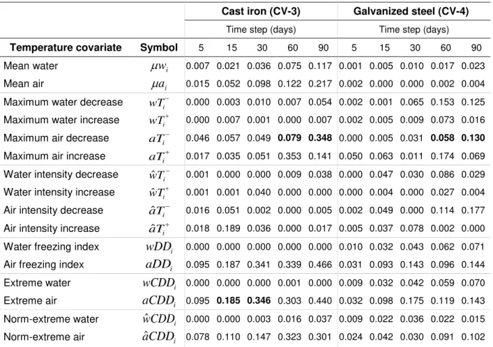
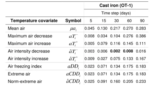
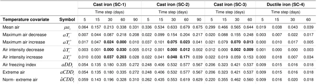
Multiple trials were conducted, using the NHP model, to examine in detail how time steps of {5, 15, 30, 60 and 90} days bare on the modeling results. These trials examined each time step, in conjunction with each covariate and with each of the seven pipe groups. As expected, these trials showed that R2 values generally improved for longer time steps (and consequently smaller total number of steps), as is demonstrated in Table 2 (CV-3, CV-4), Table 3 (OT-1), and Table 4 (SC-1, SC-2, SC-3, SC-4). The incremental improvement, however, was inconsistent; where in some trials a large improvement occurred when the time step increased from 60 to 90 days (e.g., for “maximum air decrease” covariate), while in other trials a significant improvement was obtained when the time step increased from the 15 to 30 days (e.g., for “extreme air” covariate). After a careful consideration of all the trials, a time step size of 30 days was deemed to be the best choice to balance all the conflicting arguments described above. All subsequent analyses were therefore performed using a 30 day time step.

Air and water threshold temperatures

Several (not exhaustive) trials were conducted to establish appropriate threshold values for the covariates that require threshold temperatures. These trials examined threshold values that ranged between –10oC and +15oC for air and 0oC to 10oC for water. Trials for CV-3 and CV-4 were conducted using air and water temperature-based covariates based on different air and water temperature thresholds. For all other pipe groups (OT-1, SC-1, SC-2, SC-3 and SC-4) trials were conducted using air temperature-based covariates only based on different air temperature thresholds. Table 5 provides the results of these trials. A few observations can be made:

(a) Maximum log-likelihoods (MLL) for groups CV-3 and CV-4 were not very sensitive to changes in air threshold temperatures when water temperature was kept constant at 0oC, while both MLL and R2 were quite sensitive to changes in water threshold temperature; (b) MLL and R2 for pipes from the other two utilities (groups OT-1, SC-1, SC-2, SC-3 and SC-4) were quite insensitive to changes in air threshold temperature. Careful examination of the analyses results for all pipe group indicated that the appropriate threshold temperatures are about 0oC to 1oC for air and 4oC for water (if data are available) as shown in Table 5. The insensitivity of air threshold temperatures for all pipe groups (burial depths vary between 1.2 and 2.4 m) is possibly because mains in the three utilities are buried at depths that correspond to the severity of the winters experienced (cold temperatures), e.g., Ottawa, Ontario among the three cities has the harshest winters where mains are typically buried at a depth of 2.4 m.

Temperature-based covariates

Identification of significant temperature-based covariates was done in three stages. The first two stages were used to reduce as much as possible the number of examined covariates in order to alleviate the large dimensionality inherent in the exhaustive analysis of such a multitude of covariates. A series of trials based on air temperature covariates were carried out for all pipe groups. These trials were repeated based on air and water temperature covariates for groups CV-3 and CV-4 since these groups had both air and water temperature data. The specific procedures used to identify the significant covariates are discussed below. The results of all these trials are summarized in Table 6.

In the first stage, cross-correlation matrix was obtained for the all applicable covariates to identify linear dependence between any pair of covariates. The covariates µ cf.a_i µ and w_i wDD _i cf. wCDD_i, were found to be consistently linearly dependent in pipe groups CV-3 and CV-4 (for which water temperature data were available). The covariates aDD cf._i aCDD were found to be _i consistently linearly dependent in all groups. Trials were conducted on groups CV-3 and CV-4 with covariates {µ , a_i aDD ,_i wDD } and subsequently with {_i µ , w_i aCDD_i,wCDD_i}. Results indicated that MLL and R2 were nearly identical when one set of covariates was substituted for the other. Similarly, trials were conducted on all groups, where aDD and _i aCDD were _i

covariate was adequate. Covariates identified in the first stage to be linearly dependent on other covariates are identified by shaded background in Table 6. Three covariates,µ , w_i wDD_iand

i

aCDD, were removed as candidates as a consequence of these first stage trials. After this first stage reduction, the number of remaining covariates for consideration was 13 for groups CV-3 and CV-4 and 6 for all other groups.

In the second stage, trials were only conducted for groups CV-3 and CV-4 in order to further reduce the number (13) of remaining covariates. First, the contribution of individual covariates was tested using the likelihood ratio (LR) and it was found (Table 6) that the contributions of covariates wˆT_i+ and wˆCDD_i were consistently insignificant in both groups. Next, the contribution

of these 2 covariates combined was examined, and it was found that the combined pair had a significant contribution in the cast iron pipes (CV-3) but not in the galvanized steel pipes (CV-4). Consequently, these 2 covariates (identified as “F” in Table 6) were dropped from subsequent analyses of galvanized steel pipes (CV-4) but not from analyses of cast iron pipes (CV-3). Therefore, the number of covariates to examine remained unchanged at 13 for CV-3 but was reduced to 11 for CV-4.

In the third stage, exhaustive trials were conducted for all possible combinations of the remaining covariates. The number of required trials for each group is provided in Table 6. As discussed earlier, two measures, LR test and_{R , were used to evaluate these exhaustive trials} 2 and these do not always agree. The discussion of the results is provided in two parts, namely, (1) with air and water temperature-based covariates (groups CV-3, CV-4, where both air and water temperature data were available), and (2) with only air temperature-based covariates for all groups.

Air and water temperature-based covariates: a total of 2048 (11 covariates) trials were carried out for the galvanized steel pipe in group CV-4 and evaluated using the LR tests. Three

covariates, aˆT_i−, wDD , and_i aDD , in addition to the constant _i αo, emerged as significant. The

addition of any other single, pair, triplet or more covariates was found not be significant. Eight covariates were found to be significant, i.e., contributed to incrementally increase the value ofR2 , when the same 2048 trials for CV-4 were evaluated using R . These 8 covariates include the 3 2 LR-significant covariates listed above, and the additional covariates wereµ , a_i aT_i−,aT_i+,wˆT_i−

and aˆT_i+. The value of R for the 3 LR-significant covariates was 0.33, and increased to 0.52 2 with the additional 5 covariates. Interestingly, for the entire 11 covariates the value of R was 2 0.48 (substantially lower than for the best 8 covariates, as could be expected). These results are reflected in the appropriate column in Table 6.

Some interesting observations about the 2 covariates, aˆT_i− andwDD , are noteworthy. While _i their individual contributions to the LR values were small, their contribution as a pair was very significant. Further, the sign of the coefficient for one of these covariates (wDD ) came out _i negative (rather than positive) indicating that a decrease in its value causes an increase in the number of predicted breaks, which is contrary to what might be expected (higher water freezing index, wDD_i are intuitively expected to result in elevated breakage rate). Similarly, coefficients for some of other 8 covariates identified by the R measure were also found to have signs that 2 were contrary to what one would intuitively expect. We currently do not have satisfactory explanations for these counter-intuitive results, which merit further research.

A total of 8192 trials (13 covariates) were conducted for cast iron pipe group, CV-3. Seven covariates, in addition to the constant αo, emerged as LR-significant. These 7 significant

covariates were wT_i+,wˆTi−,

+ i T

wˆ ,wDD_i, aDD_i, wˆCDD_i and aˆCDD_i. The addition of any other single, pair, triplet or more covariates was found not to be significant. It is noted that 5 of the 7 significant covariates were based on water temperature and only 2 on air temperature. The application of the R measure produced 11 significant covariates, including the 7 LR-significant 2 covariates listed above, plus: µa_i,wT_i−,aT_i+ and aˆT_i+. The value of R for the 7 LR-significant 2 covariates was 0.53, and increased to 0.65 for the 11 covariates. Interestingly, the value of R 2 was 0.62 for the entire 13 covariates which is lower (as could be expected) than for the best 11 covariates. The signs of some of the coefficients of covariates for CV-3 were found to be contrary to what might intuitively be expected, an observation which is similar to that made on galvanized steel pipes (CV-4). In particular, the sign for covariate (wDD ) came out also _i negative (rather than positive), as for group CV-4.

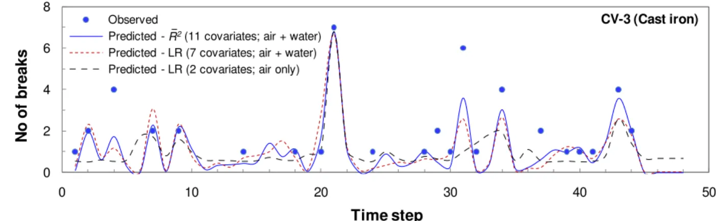
Fig. 3 and Fig. 4 compare the number of observed and predicted breaks for groups CV-3 and CV-4, respectively. It should be noted that the time step size was 30 days and that the “ageing

function” was not considered because ageing is not likely to play a significant role when the analysis period is as short as 3½ years. Fig. 3 and Fig. 4 show if both air and water temperatures are available, then the model with LR-significant covariates (7 for CV-3 and 3 for CV-4) is able to predict the observed number of breaks reasonably well. As expected, the comparison is even better with more covariates as obtained by R measure (11 for CV-3 and 8 for CV-4). 2

Air temperature-based covariates: 128 trials (7 covariates) were required for groups CV-3 and CV-4. For group CV-3, covariates aˆT_i+andaDD , in addition to the constant _i αo, emerged as

LR-significant. An additional covariate, µ , was found significant for CV-4. The addition of other a_i single or multiple covariates was found not be significant. Using the R measure, the same 2 2 covariates were found to be significant for CV-3 and 4 covariates for CV-4. These covariates include the LR-significant covariates listed above, and the additional covariate of aˆT_i− for CV-4. The values of R for the LR-significant covariates were 0.37 and 0.26 for CV-3 and CV-4, 2 respectively. Slightly higher R values were obtained for CV-3 and CV-4 when significant 2 covariates were determined using the R measure. Fig. 3 and Fig. 4 illustrate the quality of fit of 2 the model (using air temperature-based covariates only) to the observed break data for CV-3 and CV-4, respectively. The figures show that prediction of water main breaks using only air

temperature-based covariates is not as good as when both air and water temperature-based covariates are available, i.e., R values of 0.53 cf. 0.37 for CV-3 and 0.33 cf. 0.26 for CV-4 2 based on the LR test (Table 6).

Only 64 trials (6 covariates) were required for groups, OT-1, SC-1, SC-2, SC-3 and SC-4. As shown in Table 6, the same 3 covariates were found to be LR-significant for the three cast iron groups 1, 2 and 3 whereas significant covariates for groups OT-1 (cast iron) and 4 (ductile iron) were different. Four covariates were found to be significant in groups OT-1, SC-2 and SC-3 based on the _{R measure; whereas only 1 and 2 covariates were identified as} 2 significant for SC-4 and SC-1. Only 1 covariate, mean air temperature (µa_i) was found to be significant as per the R measure and LR-test in all 5 groups. 2

All these trials showed that none of the covariates was found to be consistently significant in all pipe groups when only air temperature-based covariates were considered. The trials also

showed that the 3 covariates found to be the most consistently significant were the average mean air temperature (µa_i), maximum air temperature decrease (aT_i−), and how fast the air

temperature increases over a specific period of days, i.e., aˆT_i+. Covariates that express the maximum air temperature increase (aT_i+), and how fast the air temperature decreases over a specific period of days, i.e., aˆT_i−, were also observed to be significant in 4 of the 7 pipe groups considered in this study.

The comparisons of predicted and observed number of breaks (with and without the

consideration of ageing) for OT-1 for the 30 day time step are shown in Fig. 5. Ageing is likely to have occurred over the analysis period of 18 years. Consideration of ageing increased the goodness of fit measure R from 0.25 to 0.36, which are relatively low compared to values 2 obtained for other pipe groups. It is likely that this may be due to deeper burial depth (2.4 m) of water mains in Ottawa, which would minimize the effects of frost penetration.

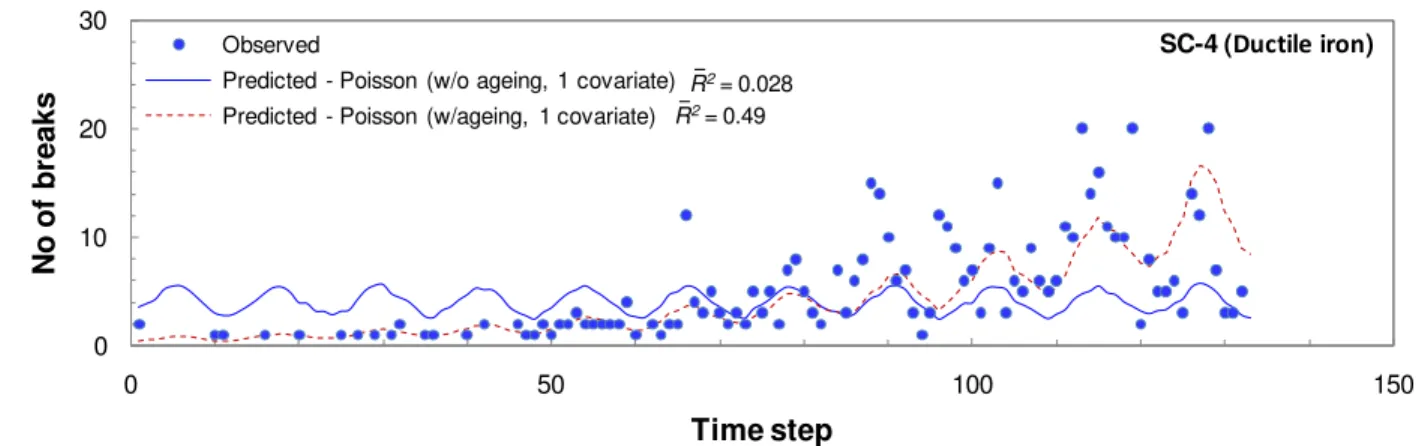
The comparison of predicted and observed number of breaks for SC-1, SC-2, SC-3 and SC-4 for the 30 day time step are shown in Fig. 6, Fig. 7, Fig. 8 and Fig. 9, respectively. In these comparisons, the ageing function was also considered in the prediction of water main breaks since ageing is likely to have occurred over the analysis period of 22 years.

The peaks and the valleys in the observed number of main breaks over the 22+ years match reasonably well with the predicted number of main breaks for all pipe groups except for SC-1 and SC-4. The match between observed and predicted number of breaks for SC-1 do not appear to be as good as that obtained for OT-1 even though comparable R values were obtained (Table 2 6). A significantly higherR value was obtained for SC-1 when the same analysis was conducted 2 using a larger time step size of 60 days instead of 30 days. It is noted that group SC-1 is a much smaller group with fewer breaks per time step (Table 6) which is likely to accentuate the issues with predicted real numbers versus observed integers for the number of breaks. As seen in Fig. 9, the number of breaks in pipe group SC-4 is largely a result of ageing, whereas temperature-based covariates appear to have only a slight impact on the number of breaks. This observation is in accordance with the fact discussed earlier that ductile iron pipes have high ductility and hence do not in general suffer physical fracture but rather fail through the development of perforations by

the onset of external corrosion which is time-dependent. This is further corroborated by the significant higher ageing coefficient obtained for SC-4 as seen in Table 6.

Final remarks

The analysis to assess the impact of temperature-based covariates suggests that water temperature-based covariates appear to have significant impact on observed breaks as indicated by much higher values ofR , obtained when both water and air temperature-based covariates are 2 used. This influence was most significant in cast iron pipes. However, only air temperature-based covariates can also explain the main breaks as shown by the high R values obtained in the trials 2 for pipe groups OT-1, SC-2 and SC-3. The same covariates are found not to be significant for all pipe groups. As many as 7 to 11 covariates and as few as 1 to 3 covariates were found to be significant, using LR and R measures as goodness of fit, respectively. 2

Three covariates, namely, average mean air temperature (µa_i), maximum air temperature increase and decrease (aT_i+,aT_i−), and how fast the air temperature increase and decrease

(intensities) over a specific period of days, i.e., aˆT_i+,aˆT_i−, were found to be the most consistently significant covariates. These covariates concur with some observations that the breakage

frequency increase when the air temperature transits from above 0oC to below 0oC or vice versa, e.g., during late fall (drop) and early spring (rise).

Signs for some of the coefficients of covariates were found to be contrary to intuitive

expectations, e.g., decrease in the intensity of air temperature change (aˆT_i−) and decrease in water freezing index (wDD ) lead to an increase in predicted breaks. It is quite plausible that _i some of these covariates work together in a manner that is different from when each covariate is considered on its own.

The availability of both air and water temperature data provided the opportunity to explore their possible influence on water main breaks in three different pipe material types. The analyses showed that different pipe materials can respond differently to air and to water temperature-based covariates. The same type of analyses conducted on data where only air temperature data are available, a typical situation since water utilities do not usually monitor water temperature, showed that some of the proposed air temperature-based covariates have a significant impact on

main breaks. The appropriate time step for analysis was identified as 30 days. Few more case studies of the type reported here may be warranted to confirm the influence of water

temperature-based covariates on water main breaks.

Acknowledgement

This paper is based on a research project, which was co-sponsored by the Water Research Foundation, the National Research Council of Canada (NRC) and American Water from the United States. Mr. David Hughes from American Water led the effort towards the collection of data for Connellsville and his help is duly acknowledged.

References

Ahn, J.C., Lee, S.W., Lee, G.S. and Koo, J.Y. (2005). “Predicting water pipe breaks using neural network.” Water Science and Technology: Water Supply, 5(3-4), 159-172.

Bahmanyar, G. H. and Edil, T. B. (1983). “Cold weather effects on underground pipeline failures.” Proceedings of Conference on Pipelines in Adverse Environments II, ASCE, San Diego, CA. Mark B. Pickell, (ed). pp. 579-593.

Cocks, R. and Oakes, A. (2011). “Modelling the impact of weather on leakage and bursts.” Computing and Control in the Water Industry 2011: Urban Water Management: Challenges and Opportunities, University of Exeter, England.

Constantine, A. G. and Darroch, J. N. (1993). “Pipeline reliability: stochastic models in engineering technology and management.” S. Osaki and D.N.P. Murthy (eds). World Scientific Publishing Co.

Constantine, A. G., Darroch, J. N. and Miller, R. (1996). “Predicting underground pipe failure.” Australian Water Works Association.

Economou, T., Kapelan, Z. and Bailey, T. (2008). “A zero-inflated Bayesian model for the prediction of water pipe bursts”, Proc. 10th International Water Distribution System Analysis Conference, CD-ROM edition, Kruger National Park, South Africa.

Goodchild, C.W., Rowson, T.C. and Engelhardt, M.O. (2009). “Making the earth move: Modelling the impact of climate change on water pipeline serviceability.” Computing and Control in the Water Industry 2009: Integrating Water Systems, University of Sheffield, England. J. Boxall and C. Maksimovic (eds). pp. 807-811.

Habibian, A. (1994). “Effect of temperature changes on water-main break.” Journal Transportation Engineering, ASCE, 120(2), 312-321.

Hughes, D., Kleiner, Y., Rajani, B. and Sink, J-E. (2010). “Continuous system acoustic monitoring - from start to repair.” Water Research Foundation, Denver, CO. (in print). Kleiner, Y. and Rajani, B. (2003). “Forecasting variations and trends in water-main breaks.” Journal of Infrastructure Systems, ASCE, 8(4), 122-131.

Kleiner, Y. and Rajani, B. (2004). “Quantifying effectiveness of cathodic protection in water mains: theory.” Journal of Infrastructure Systems, ASCE, 10(2), 43-51.

Kleiner, Y. and Rajani, B. (2009). “I-WARP: individual water main renewal planner.”

Computing and Control in the Water Industry 2009: Integrating Water Systems, University of Sheffield, England. J. Boxall and C. Maksimovic (eds). pp. 639-644.

Lochbaum, B. S. (1993). “PSE&G develops models to predict main breaks.” Pipeline and Gas Journal, 20(9), 20-27.

Miller, R. B. (1993). “Personal communications”. CSIRO Division of Mathematics and Statistics, Glen Osmond. Australia.

Newport, R. (1981). “Factors influencing the occurrence of bursts in iron water mains.” Water Supply and Management, 3, 274-278.

Røstum, J. (2000). “Statistical modelling of pipe failures in water networks”. PhD thesis, Norwegian University of Science and Technology, Trondheim, Norway.

Sacluti, F., Stanley, S. J. and Zhang, Q. (1999). “Use of artificial neural networks to predict water distribution pipe breaks.” Western Canada Water and Wastewater Association, 50th Annual Conference, Calgary, Alberta.

Walski, T. M. and Pelliccia, A. (1982). “Economic analysis of water main breaks.” Journal American Water Works Association, 74(3), 140-147.

(a) 2 day time step

(b) 5 day time step

(c) 15 day time step

(d) 30 day time step

Fig. 1. Time histories for number of main breaks, mean air and water temperatures for different time step sizes – galvanized steel (Group CV-4).

-20 -10 0 10 20 30 0 2 4 6 8 0 10 20 30 40 50 C o var iat e N o of br e a k s Time step

Breaks - Obvs. Mean water T Mean air T -20 -10 0 10 20 30 0 2 4 6 0 20 40 60 80 100 C o var iat e N o of br e a k s Time step

Breaks - Obvs. Mean water T Mean air T -20 -10 0 10 20 30 0 1 2 3 4 0 100 200 300 400 500 600 700 C o var iat e N o of br e a k s Time step

Breaks - Obvs. Mean water T Mean air T

-20 -10 0 10 20 30 0 1 2 3 4 0 50 100 150 200 250 300 C o var iat e N o of br e a k s Time step

(a) 2 day time step

(b) 5 day time step

(c) 15 day time step

(d) 30 day time step

Fig. 2. Time histories for number of main breaks, mean air and water temperatures for different time step sizes – cast iron (Group SC-2).

-30 -15 0 15 30 0 2 4 6 8 10 0 500 1000 1500 2000 2500 3000 3500 4000 4500 C o var iat e N o of br e a k s Period

Breaks - Obvs. Mean air T

-30 -15 0 15 30 0 2 4 6 8 10 0 300 600 900 1200 1500 C o var iat e N o of br e a k s Period

Breaks - Obvs. Mean air T

-30 -15 0 15 30 0 10 20 30 0 100 200 300 400 500 600 C o var iat e N o of br e a k s Period

Breaks - Obvs. Mean air T

-30 -15 0 15 30 0 10 20 30 0 100 200 300 C o var iat e N o of br e a k s Period

Fig. 3. Comparison of observed and predicted number of breaks per time step – CV-3 (cast iron pipes).

Fig. 4. Comparison of observed and predicted number of breaks per time step – CV-4 (galvanized steel pipes).

Fig. 5. Comparison of observed and predicted number of breaks per time step – OT-1 (cast iron pipes). 0 2 4 6 8 0 10 20 30 40 50 N o of br e a k s Time step Observed

Predicted - (8 covariates; air + water) Predicted - LR (3 covariates; air + water) Predicted - LR (3 covariates; air only)

CV-4 (Galvanized steel) R2 0 2 4 6 8 0 10 20 30 40 50 N o of br e a k s Time step Observed

Predicted - (11 covariates; air + water) Predicted - LR (7 covariates; air + water) Predicted - LR (2 covariates; air only)

CV-3 (Cast iron) R2 0 5 10 15 20 0 50 100 150 200 N o of br e a k s Time step Observed

Predicted - Poisson (w/o ageing, 3 covariates) Predicted - Poisson (w/ageing, 3 covariates)

OT-1 (Cast iron₎

R2_{= 0.25}

Fig. 6. Comparison of observed and predicted number of breaks per time step – SC-1 (cast iron pipes).

Fig. 7. Comparison of observed and predicted number of breaks per time step – SC-2 (cast iron pipes).

Fig. 8. Comparison of observed and predicted number of breaks per time step – SC-3 (cast iron pipes). 0 10 20 30 40 50 0 50 100 150 200 250 N o of br e a k s Time step Observed

Predicted - Poisson (w/o ageing, 3 covariates) Predicted - Poisson (w/ageing, 3 covariates)

SC-3 (Cast iron₎ R2_{= 0.67} R2_{= 0.58} 0 10 20 30 40 0 50 100 150 200 250 N o of br e a k s Time step Observed

Predcited - Poisson (w/o ageing, 3 covariates) Predcited - Poisson (w/ageing, 3 covariates)

SC-2 (Cast iron₎ R2_{= 0.74} R2_{= 0.64} 0 4 8 0 50 100 150 200 250 N o of br e a k s Time step Observed

Predicted - Poisson (w/o ageing, 2 covariates) Predicted - Poisson (w/ageing, 2 covariates)

SC-1 (Cast iron₎

R2_{= 0.22}

Fig. 9. Comparison of observed and predicted number of breaks per time step – SC-4 (ductile iron pipes). 0 10 20 30 0 50 100 150 N o of br e a k s Time step Observed

Predicted - Poisson (w/o ageing, 1 covariate) Predicted - Poisson (w/ageing, 1 covariate)

SC-4 (Ductile iron)

R2_{= 0.49}

Table 1. Characteristics of homogenous pipe groups used in this research.

Connellsville Ottawa Scarborough

Pipe groups CV-3 CV-4 OT-1 SC-1 SC-2 SC-3 SC-4

Pipe material cast iron

(Pit) galvanized steel cast iron (spun) cast iron (pit) cast iron (spun) cast iron (spun) ductile iron

Pipe diameter (in) 2 ½-12” 2 - 2½” 6” 6” 6” 6” 6”

Vintage ~ 1880s ~ 1880s 1954-74 1921-35 1943-55 1956-78 1960-83

Burial depth (m) 1.2 2.4 1.5

Break years 2005-08 2005-08 1972-89 1962-83 1962-83 1962-83 1970-83

Pipe length (km) n/a n/a 230 66 424 748 186

No of breaks 48 88 1,033 211 1,677 3,045 538

Average break

rate (/100 km/year) n/a n/a 25 14.5 18 18.5 13.1

Table 2. Goodness of fit (R ) values for different time step size – Connellsville 2

Cast iron (CV-3) Galvanized steel (CV-4)

Time step (days) Time step (days)

Temperature covariate Symbol 5 15 30 60 90 5 15 30 60 90 Mean water 0.007 0.021 0.036 0.075 0.117 0.001 0.005 0.010 0.017 0.023 Mean air µa_i 0.015 0.052 0.098 0.122 0.217 0.002 0.000 0.000 0.002 0.004 Maximum water decrease wT_i− 0.000 0.003 0.010 0.007 0.054 0.002 0.001 0.065 0.153 0.125 Maximum water increase wT_i+ 0.000 0.007 0.001 0.000 0.007 0.002 0.005 0.009 0.073 0.016 Maximum air decrease aT_i− 0.046 0.057 0.049 0.079 0.348 0.000 0.005 0.031 0.058 0.130 Maximum air increase aT_i+ 0.017 0.035 0.051 0.353 0.141 0.050 0.063 0.011 0.174 0.069 Water intensity decrease wˆT_i− 0.001 0.000 0.000 0.009 0.038 0.000 0.047 0.030 0.086 0.029 Water intensity increase wˆT_i+ 0.001 0.001 0.040 0.000 0.000 0.000 0.004 0.000 0.027 0.004 Air intensity decrease aˆT_i− 0.016 0.051 0.002 0.000 0.005 0.002 0.049 0.000 0.114 0.177 Air intensity increase aˆT_i+ 0.018 0.189 0.036 0.000 0.017 0.005 0.037 0.078 0.002 0.000 Water freezing index wDD_i 0.000 0.000 0.000 0.000 0.000 0.010 0.032 0.043 0.062 0.071 Air freezing index aDD_i 0.095 0.187 0.341 0.339 0.466 0.031 0.093 0.143 0.096 0.144 Extreme water wCDD_i 0.000 0.000 0.000 0.001 0.000 0.009 0.032 0.042 0.059 0.070 Extreme air aCDD_i 0.095 0.185 0.346 0.303 0.440 0.032 0.098 0.175 0.119 0.143 Norm-extreme water wˆCDD_i 0.000 0.000 0.003 0.016 0.037 0.009 0.022 0.036 0.022 0.015 Norm-extreme air aˆCDD_i 0.078 0.110 0.147 0.323 0.301 0.024 0.042 0.030 0.091 0.102

Bold font indicates large changes in R2 values.

i w

Table 3. Goodness of fit (R ) values for different time step size – Ottawa 2

Cast iron (OT-1)

Time step (days)

Temperature covariate Symbol 5 15 30 60 90 Mean air µa_i 0.045 0.130 0.217 0.270 0.283 Maximum air decrease aT_i− 0.008 0.034 0.104 0.276 0.386 Maximum air increase aT_i+ 0.005 0.079 0.116 0.145 0.111 Air intensity decrease aˆT_i− 0.003 0.006 0.002 0.008 0.016 Air intensity increase aˆT_i+ 0.009 0.027 0.075 0.133 0.167 Air freezing index aDD_i 0.023 0.071 0.134 0.175 0.183 Extreme air aCDD_i 0.023 0.071 0.134 0.175 0.183 Norm-extreme air aˆCDD_i 0.025 0.091 0.160 0.205 0.233