Risk-based prioritization of air pollution monitoring using fuzzy synthetic evaluation technique

Publisher’s version / Version de l'éditeur:

Environmental Monitoring and Assessment, 105, June, pp. 261-283, 2005-06-01

READ THESE TERMS AND CONDITIONS CAREFULLY BEFORE USING THIS WEBSITE.

https://nrc-publications.canada.ca/eng/copyright

Vous avez des questions? Nous pouvons vous aider. Pour communiquer directement avec un auteur, consultez la

première page de la revue dans laquelle son article a été publié afin de trouver ses coordonnées. Si vous n’arrivez pas à les repérer, communiquez avec nous à PublicationsArchive-ArchivesPublications@nrc-cnrc.gc.ca.

Questions? Contact the NRC Publications Archive team at

PublicationsArchive-ArchivesPublications@nrc-cnrc.gc.ca. If you wish to email the authors directly, please see the first page of the publication for their contact information.

NRC Publications Archive

Archives des publications du CNRC

This publication could be one of several versions: author’s original, accepted manuscript or the publisher’s version. / La version de cette publication peut être l’une des suivantes : la version prépublication de l’auteur, la version acceptée du manuscrit ou la version de l’éditeur.

For the publisher’s version, please access the DOI link below./ Pour consulter la version de l’éditeur, utilisez le lien DOI ci-dessous.

https://doi.org/10.1007/s10661-005-3852-1

Access and use of this website and the material on it are subject to the Terms and Conditions set forth at Risk-based prioritization of air pollution monitoring using fuzzy synthetic evaluation technique

Khan, F. I.; Sadiq, R.

https://publications-cnrc.canada.ca/fra/droits

L’accès à ce site Web et l’utilisation de son contenu sont assujettis aux conditions présentées dans le site

LISEZ CES CONDITIONS ATTENTIVEMENT AVANT D’UTILISER CE SITE WEB.

NRC Publications Record / Notice d'Archives des publications de CNRC: https://nrc-publications.canada.ca/eng/view/object/?id=3f3dd3c6-668b-4071-aab4-148df1d5673f https://publications-cnrc.canada.ca/fra/voir/objet/?id=3f3dd3c6-668b-4071-aab4-148df1d5673f

Risk-based prioritization of air pollution monitoring using fuzzy synthetic evaluation technique

Khan, F.I.; Sadiq, R.

NRCC-47731

A version of this document is published in / Une version de ce document se trouve dans : Environmental Monitoring and Assessment, v. 105, no. 1-3, June 2005, pp. 261-283

DOI:10.1007/s10661-005-3852-1

Risk-based prioritization of air pollution monitoring using fuzzy

synthetic evaluation technique

Faisal I. Khan1* and Rehan Sadiq2 1

Faculty of Engineering & Applied Science, Memorial University of Newfoundland, St. John’s, NL, Canada

2

Institute for Research in Construction, National Research Council, Ottawa, ON, Canada

*

Correspondence author: fkhan@engr.mun.ca ABSTRACT

Air pollution monitoring programs aim to monitor pollutants and their probable adverse effects at various locations over concerned area. Either sensitivity of receptors/location or concentration of pollutants is used for prioritising the monitoring locations. The exposure-based approach prioritises the monitoring locations based on population density and/or location sensitivity. The hazard-based approach prioritises the monitoring locations using intensity (concentrations) of air pollutants at various locations. Exposure and hazard-based approaches focus on frequency (probability of occurrence) and potential hazard (consequence of damage), independently. Adverse effects should be measured only if receptors are exposed to these air pollutants. The existing methods of monitoring location prioritization do not consider both factors (hazard and exposure) at a time. Towards this, a risk-based approach has been proposed which combines both factors: exposure frequency (probability of occurrence/exposure) and potential hazard

(consequence).

This paper discusses the use of fuzzy synthetic evaluation technique in risk computation and prioritization of air pollution monitoring locations. To demonstrate the application, common air pollutants like CO, NOx, PM10 and SOx are used as hazard parameters. Fuzzy evaluation matrices for hazard parameters are established for different locations in the area. Similarly, fuzzy evaluation matrices for exposure parameters: population density, location and population

sensitivity are also developed. Subsequently, fuzzy risk is determined at these locations using fuzzy compositional rules. Finally, these locations are prioritised based on defuzzified risk (crisp value of risk, defined as risk score) and the five most important monitoring locations are

identified (out of 35 potential locations). These locations differ from the existing monitoring locations.

1. INTRODUCTION

There is substantial and consistent evidence of an association between increased levels of ambient air pollution and mortality rates. A principal hypothesis is that exposure to air pollutants may cause acute pulmonary disease, such as bronchiolitis or pneumonia, thereby leading to congestive heart failure (CHF) in persons with myocardial damage or cardiac disease

(Bates,1992). Alternatively, exposure to ultra fine particles may invoke alveolar inflammation, release inflammatory mediators, exacerbate lung conditions, and increase coagulability of blood thereby leading to acute episodes of cardiovascular disease (Seaton et al., 1995). In the recent studies, it was found that daily hospitalization cases for CHF and daily mortality among persons with CHF, increased when levels of ambient particles and gaseous pollutants are increased (Burnett et al., 1997; Morri and Naumova, 1998; Kwon et al., 2001). Goldberg et al. (2003) recently conducted a mortality time series study to investigate the relationship between daily mortality due to CHF, and concentrations of particles and gaseous pollutants in the ambient air of Montreal, Quebec, during the period 1984 –1993. They observed that CHF has a positive

correlation with coefficient of haze, extinction coefficient, SO2, and NO2. For example they reported that either an increase of 4.32% in the coefficient of haze, or 4.08% increase in NO2 concentration causes a consistent average increase in daily mortality.

Existing methods of establishing ambient air quality monitoring networks typically evaluate only parameters related to ambient concentrations of pollutant(s) such as emission source characteristics, atmospheric transport and dispersion, secondary reactions, deposition characteristics, and local topography. The objective of these monitoring network design methods is to identify the locations of maximum air pollutant concentrations (Harrison and Deacon, 1998; Bladauf et al., 2001, 2002). However, toxicological and epidemiological studies indicate that adverse health effects from exposures to airborne contaminants are also a function of the characteristics of the individuals exposed to the pollutant. Children, the elderly, healthy adults, and diseased adults can tolerate different pollutant concentration levels before experiencing adverse health impacts (see Bladauf et al., 2001,2002; Goldberg et al., 2003 for details). Thus, the existence of high concentrations of an air contaminant will not inherently result in adverse health effects unless individuals exposed to the contaminant are susceptible at that concentration level. Ambient air quality monitoring networks designed for the protection of susceptible

population or for epidemiological studies evaluating adverse health impacts of ambient air contaminants need to account for both contaminant characteristics and human health parameters to adequately assess health risks to the exposed population.

One of the first works in this direction is by Baldauf et al. (2001). They have proposed an ambient air quality network using risk assessment techniques. In their recent work (Baldauf et al. 2002) the proposed risk assessment based method was compared with traditional methods of establishing air quality monitoring networks: identifying maximum concentration impacts or maximum total population. Results suggest that the health risk method best predicted the location of adverse, non-carcinogenic respiratory illness during the evaluation period.

Inspired by the work of Baldauf and coworkers the authors have developed a new risk-based methodology for air quality monitoring location prioritization. This paper presents the methodology, which optimizes ambient air quality monitoring locations for the assessments of adverse human-health impacts from exposures to airborne contaminants. Risk is focal point of this methodology. Rowe (1977) defines risk as the potential for unwanted negative consequences

of an event and activity, whereas Lowrence (1976) defines it as a measure of probability and severity of negative adverse effects. In this context, risk analysis is the estimation of the

frequency and physical consequences of undesirable events, which can produce harm (Ricci et al., 1981). In conclusion risk refers to the combination of event’s probabilities of occurrence and its consequences. When a complex system involves various contributory risk items with

uncertain sources and magnitudes, it often can not be treated with mathematical rigor during the initial or screening phase of decision-making (Lee, 1996).

The use of risk assessment as the basis for designing ambient air quality monitoring networks will help to target limited financial and human resources to evaluate human health risks from exposures to airborne contaminants. The monitoring network has been proposed to allow an assessment of human health risks posed by exposures to single or multiple pollutants. Predicted concentration measurements will be used to extrapolate potential health risks to the local population from exposures to these contaminants. Risk assessment methods are used to estimate adverse health effects from the anticipated exposures. Thus, monitoring sites will be established at locations that represent the maximum health risk to the surrounding population. In the present approach, risk assessment methods have been coupled with fuzzy synthetic

evaluation techniques. Risk quantification using fuzzy synthetic evaluation techniques enables propagation and dilution of uncertainties in the results. Therefore, use of this approach in

quantification of risk (due to exposure of air borne pollutants) and subsequent prioritization of air quality monitoring locations would enhance the reliability of the results.

1.1 AIR QUALITY INDEX

Two types of air pollution standards are implemented to maintain good air quality.

Primary standards are designed to establish limits to protect public health, including the health of sensitive populations, whereas, secondary standards set limits to protect public welfare, including protection against decreased visibility and damage to animals, crops, vegetation, and buildings.

Air quality indices are developed to provide overall (aggregated) information about air quality. They hint how clean or polluted the air is, and which associated health effects might be of concern. The concentrations of the major pollutants are monitored and subsequently are converted into an index using standard formulas. The US EPA reports air quality based on five major air pollutants - ozone, particulate matter, carbon monoxide, sulfur dioxide, and nitrogen dioxide. The higher value of an index refers to a greater level of air pollution and consequently higher health concerns. The US EPA divided air quality index into six categories:

(1) Good (0-50) - and air pollution poses little or no risk;

(2) Moderate (51-100) - air quality is acceptable; however, for sensitive population may experience health concerns;

(3) Unhealthy-I (101-150) - sensitive groups may experience health effects;

(4) Unhealthy-II (151-200) - everyone may begin to experience some health problems; (5) Very unhealthy (201 to 300) - everyone may experience more serious health effects; and (6) Hazardous (> 300) warning of emergency conditions and entire population is more likely

to be affected.

1.2 ENVIRONMENTAL AND HEALTH EFFECTS

Air quality deterioration may cause severe adverse environmental and health effects locally, regionally and/or globally as discussed earlier. Common environmental effects are acid rain, global warming (greenhouse gases), and ozone depletion. Two main types of human health

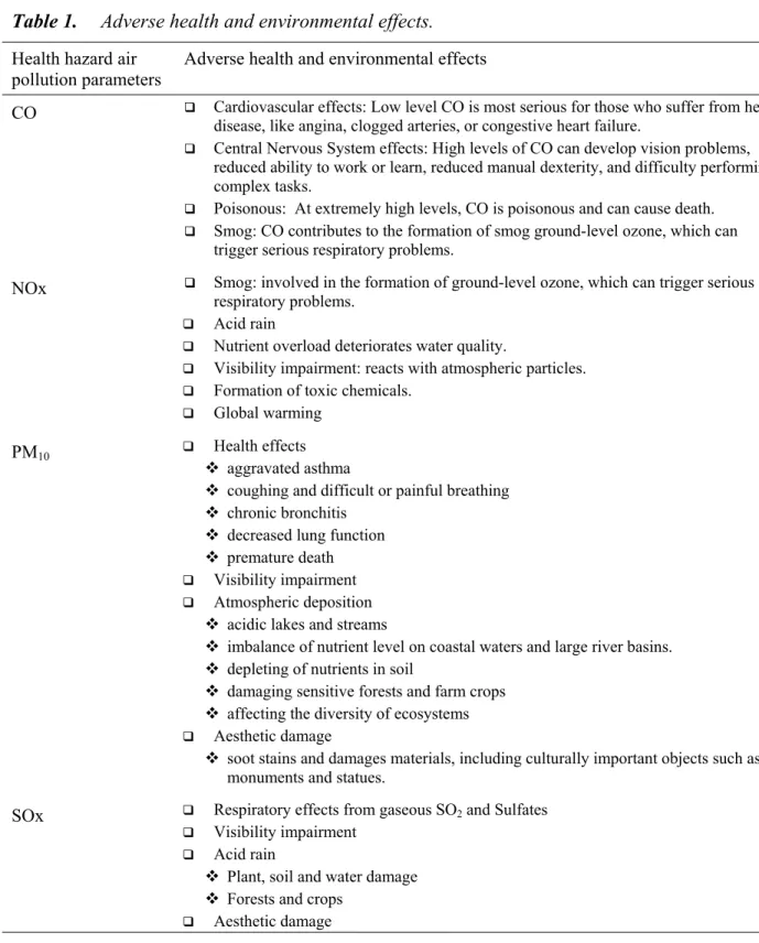
effects reported are – short term and long term effects. These effects vary from simple coughing to respiratory and cardiovascular illnesses. Table 1 lists common environmental and health impacts associated with CO, NOx, PM10 and SOx.

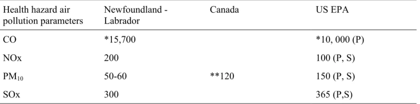
To maintain acceptable air quality, various regulatory agencies including US EPA and Health Canada have promulgated air quality standards for NOx, CO, PM10 and SOx. These standards depend on exposure time, e.g., 1-hour, 8-hours, daily, weekly, monthly and yearly averages. Table 2 summarizes the daily (24-hours) standard values for NOx, PM10 and SOx, and 8-hours average for CO.

In the next section, fundamentals of fuzzy set theory are presented. The proposed fuzzy synthetic evaluation technique for air quality monitoring is described in Section 3. Application of the proposed methodology is presented in Section 4. Section 5 discusses the benefits and

limitations of the proposed methodology as well as recommendations for future research. Summary and conclusions of this research are provided in Section 6.

2. FUZZY SETS AND SOFT COMPUTING

The term soft computing describes an array of emerging techniques such as fuzzy logic, probabilistic reasoning, neural networks, and genetic algorithms. All these techniques are essentially heuristic which provide rational solutions for complex real-world problems

(Bonissone, 1997). Quantitative aggregation of risk due to various sources is a complex process which warrants such an approach.

Fuzzy logic provides a language with syntax and semantics to translate qualitative knowledge into numerical reasoning. In many engineering problems, information about the probabilities of various risk items is vaguely known or assessed. The term computing with words has been introduced by Zadeh (1996) to explain the notion of reasoning linguistically rather than with numerical quantities. Such reasoning has a central importance for many emerging

technologies related to engineering and applied sciences. This approach has proved very useful in medical diagnosis (Lascio et al., 2002), information technology (Lee, 1996), water quality assessment (Lu et al., 1999; Lu and Lo, 2002; Sadiq et al., 2004a), corrosion of cast iron pipes (Sadiq et al., 2004b) and in many other industrial applications (Lawry, 2001).

When evaluating risk items in complex systems, decision-makers, engineers, managers, regulators and other stake-holders often view risk in terms of linguistic variables like very high,

high, very low, low etc. The fuzzy set theory is able to deal effectively with these types of

uncertainties (encompassing vagueness), and linguistic variables can be used to approximate reasoning and can be subsequently manipulated to propagate uncertainties throughout the decision process. Fuzzy-based techniques are a generalized form of interval analysis used to address uncertain and/or imprecise information. A fuzzy number describes the relationship between an uncertain quantity x and a membership function µ, which ranges between 0 and 1. A fuzzy set is an extension of the traditional set theory (in which x is either a member of set A or not) in that an x can be a member of set A with a certain degree of membership µ. Fuzzy-based techniques can help in addressing deficiencies inherent in binary logic and are useful in

propagating uncertainties through models. Any shape of a fuzzy number is possible, but the selected shape should be justified by available information. Generally, triangular fuzzy numbers or trapezoidal fuzzy numbers are used for representing linguistic variables (Lee, 1996).

Defuzzification is a process to evaluate a crisp or point estimate of a fuzzy number. A

defuzzified number is generally represented by the centroid, often determined using the centre of area method (Yager, 1980).

Fuzzy set theory has been used for classification of rivers since the 1980s. The majority of research in environmental modeling (specifically water quality modeling) has been focused on fuzzy synthetic evaluation (FSE) and fuzzy clustering analysis (FCA). The FSE is used to

classify samples at a known centre of classification (or group), whereas the FCA is used to classify samples according to their relationships when this centre is unknown (Lu et al., 1999). The FSE classifies samples for known standards and guidelines, which is a modified version of traditional synthetic evaluation techniques. In this paper the FSE technique is used in developing the framework for prioritization of air pollution monitoring locations.

3. THE PROPOSED METHODOLOGY WITH FUZZY SYNTHETIC EVALUATION TECHNIQUE This section describes the proposed methodology to prioritize ambient air quality

monitoring locations based on assessments of risk from the exposures to airborne contaminants. The concept of risk is the main thrust for this methodology. The architecture of the proposed

methodology is shown in Figure 1. The methodology involves six main steps, which are detailed in subsequent subsections.

In the fuzzy domain, risk is a composition of two fuzzy sets – likelihood (exposure) and hazard. It is equivalent to defining risk as the joint probabilities of occurrence and consequences provided the representative probabilities are independent. In this paper, indices for both exposure and hazard are established using fuzzy synthetic evaluation techniques and then compositional rules are established to determine fuzzy risk. Fuzzy-based approaches involve three main steps: determination of performance scores (for different pollutants or exposure parameters); grouping (aggregation) of attributes; and ranking according to aggregated scores. These three steps are referred to as fuzzification, aggregation and defuzzification, respectively (see Figure 1).

3.1. STEP 1 - DEVELOPMENT OF MEBERSHIP FUNCTIONS

Three linguistic variables (fuzzy subsets) are defined using triangular fuzzy numbers (TFNs) for exposure and hazard parameters. The granularity (number of qualitative levels or fuzzy subsets) is an expert’s or an industry’s choice, which may be defined in three to eleven qualitative levels. Consensus needs to be established among the experts on the issue of defining shapes of fuzzy sets for each basic attribute. The experts may include practitioners, regulators, and researchers. In the present study, experts agreed to define heuristically three granulars (or fuzzy subsets) – low, medium, high –to maintain simplicity in the analysis.

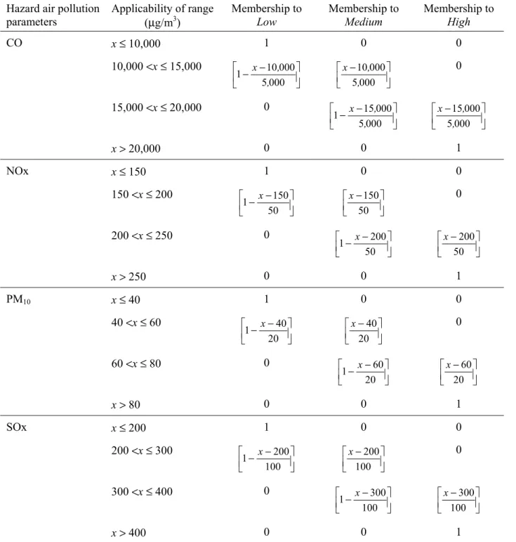
Four hazard and three exposure (likelihood) parameters were identified. Air pollution hazard parameters include - CO, NOx, PM10 and SOx. Exposure parameters include location sensitivity (LS), population density (PD), and population sensitivity (PS). Table 3 defines the TFN for each linguistic variable defined for CO, NOx, PM10 and SOx. The membership function (µ) for each linguistic variable is defined with the help of regulatory values provided in Table 2. For example for CO, the membership to low fuzzy subset ( ) is assigned a value 1 for

concentration less than 10

L CO

µ

CO

4_µ

g/m3. The membership decreases linearly and becomes 0 at 1.5×104

µg/m3. But, at this value membership to medium ( ) becomes 1 and membership assigned to

high fuzzy subset ( ) is 0. After 1.5×10

M CO µ H CO µ 4_µ

g/m3, the decreases linearly and becomes 0 at 2×10

M

µ 4_µ

becomes 1 at 2×104µg/m3 and remains constant after that. Therefore, any value over the universe of discourse of CO can be defined by a 3-tuple fuzzy set [ ]. Similarly, the membership functions for other health hazard parameters are also defined as given in Table 3. L CO µ M CO µ H CO µ

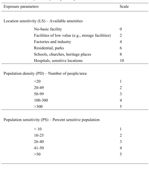
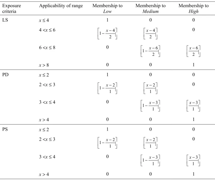
Table 4 provides details of three exposure parameters – location sensitivity (LS), population density (PD), and population sensitivity (PS). The LS refers to the importance of various areas with respect to their potential use. A scale is defined over a range of 0-10. The higher the score the more sensitive is the area. For example, hospitals and nursing homes are rated highly sensitive locations and assigned a value of 10. A value of 0 is assigned to a location where no infrastructure facility is present. Similarly, for population density a scale varying from 1-5 is defined which refers to population per unit area. Higher population density refers to higher values as an exposure parameter. Population sensitivity is also defined on a scale of 1-5. The highest value of 5 is assigned to a population with more than 50% vulnerable inhabitants (age below 18 and/or age above 60 years). These numerical values for various exposure parameters are converted into linguistic variables - low, medium and high. Each linguistic variable is defined by TFN as given in Table 5.

3.2. STEP 2 - FUZZIFICATION

The fuzzification process converts parameters (of the same or different units) into a homogeneous scale by assigning memberships with respect to predefined linguistic variables. Fuzzification maps any value of parameter on to fuzzy subsets, which are expressed by a 3-tuple fuzzy set

[

procedure follows that a value of each attribute is mapped on to a corresponding scale and the memberships to each fuzzy subset are determined where it intersects the scale. An example is shown in Figure 2 in which the universe of discourse X is defined. The observed input value for a parameter is x

]

]

1. When x1 is mapped on universe of discourse X, the 3-tuple fuzzy set

is obtained, where numbers account for the memberships to fuzzy subsets low,

medium and high, respectively. The values in a 3-tuple fuzzy set imply that x

[

the fuzzy subset high, but has a certain memberships to low (0.7) and medium (0.3) fuzzy subsets.

3.3. STEP 3 - ANALYTIC HIERARCHY PROCESS (AHP) – WEIGHTING SCHEME

Fuzzy synthetic evaluation requires information on the relative importance of parameters. The relative importance is established by a set of preference weights which can be normalized to a sum of 1. In the case of n attributes, a set of weights can be written as:

) w ,..., w , w ( W = _{1 2 n} where ∑ = (1) = n j j w 1 1

Saaty (1988) proposed an analytic hierarchy process (AHP) to estimate the relative importance of each attribute (in a group) using pair-wise comparisons. Lu et al. (1999), Sadiq et

al. (2004b), and Khan et al. (2002) have used this technique for calculating the weights for

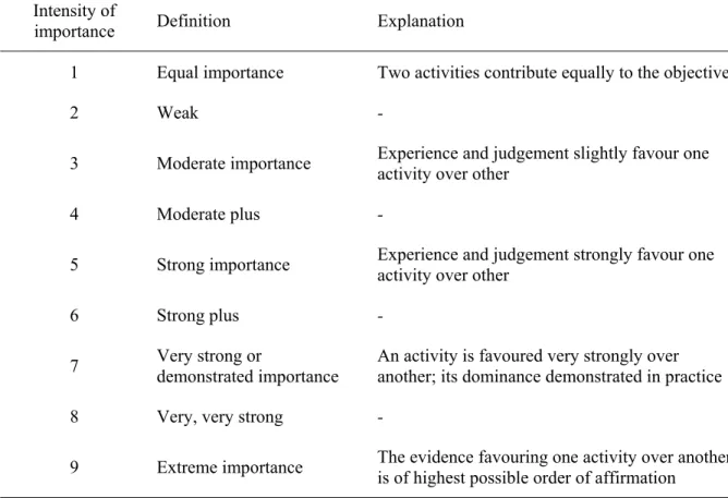
different attributes in decision-making systems. The relative importance of different factors is assigned using the intensity of importance as given in Table 6. An importance matrix J can be established where each element jmn in the upper triangular matrix expresses the importance

intensity of an attribute m with respect to another attribute n. For example, in the importance matrix J below, hazard parameter CO has been assigned importance intensities 1/3, 1/2 and 2/3 with respect to NOx, PM10 and SOx, respectively. Each element in the lower triangle of the matrix is the reciprocal of the upper triangle, i.e., jnm = 1/jmn. The importance matrix J was thus

developed as an example: CO NOx PM10 SOx CO _{1.00 0.33 0.50 0.67} J = NOx _{3.00 1.00 0.50 0.50 (2)} PM10 2.00 2.00 1.00 0.50 SOx _{1.50 2.00 2.00 1.00}

The value of each element jmn in J above is assigned based on expert opinion and

judgement. As mentioned earlier, experts include practitioners, regulators, and researchers working on environmental issues related to processing industries and thermal power plants. A

matrix I can be determined by taking the geometric mean of each row and then the weighted vector W can be derived by normalization of matrix I.

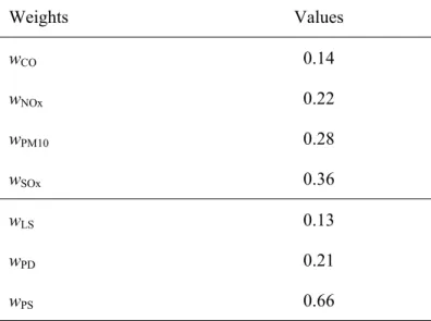
            =             = ⇒             = 36 0 28 0 22 0 14 0 57 1 19 1 93 0 58 0 10 . . . . w w w w W . . . . I SOx PM NOx CO Haz (3)

Similarly, the vector WExp is established using the same procedure (see Table 7). The final weights for exposure parameters are given below

          =           = 66 0 21 0 13 0 . . . w w w W PS PD LS Exp (4)

3.4. STEP 4 – AGGREGATION OF HAZARD AND EXPOSURE FUZZY SETS

After fuzzification and determination of weights, the exposure and hazard parameters are aggregated using matrix multiplication. As there are four hazard parameters, each parameter is multiplied by its corresponding weight to determine the cumulative 3-tuple fuzzy set for hazard

H =

[

]

]

Similarly, exposure parameters are aggregated to obtain a cumulative 3-tuple fuzzy set for exposure E

E =

[

H PS M PS L PS H PD M PD L PD H LS M LS L LS PS PD LS w w w µ µ µ µ µ µ µ µ µ µ µ µ =           ×          

3.5. STEP 5 – DETERMINATION OF RISK

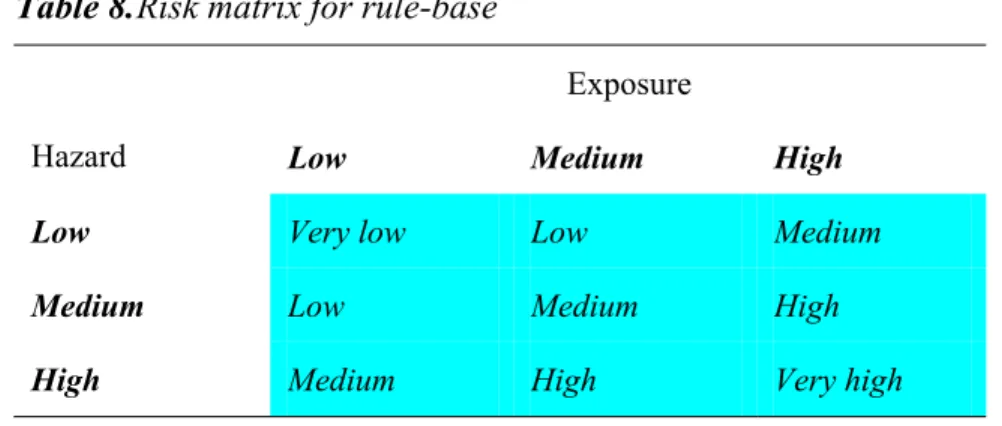
Fuzzy risk is a composition of hazard and exposure fuzzy sets. In this paper, risk is defined as a 5-tuple fuzzy set – very low, low, medium, high and very high. The following rule-base is established to determine the fuzzy risk:

If hazard is low and exposure is low then risk is very low

If hazard is low and exposure is medium then risk is low If hazard is medium and exposure is low then risk is low

If hazard is low and exposure is high then risk is medium

If hazard is medium and exposure is medium then risk is medium If hazard is high and exposure is low then risk is medium If hazard is medium and exposure is high then risk is high If hazard is high and exposure is medium then risk is high If hazard is high and exposure is high then risk is very high

The above nine rules are also presented in Table 8 in a matrix form. In the fuzzy

composition, various aggregation operators can be used in sequences compositional rule refers to a specific sequence of aggregation operations (Klir and Yuan, 1995). Based on these rules, the composition for fuzzy risk can be explained as

(

)

(

) (

)

(

) (

) (

)

(

) (

)

(

)

The signs

⊗

⊕

minimum. Similarly, the or-type operators are sum and maximum. Therefore the common types of inferencing in fuzzy composition are sum-product and max-min rules. Both composition rules are used in this research.

3.6. STEP 6 – DEFUZZIFICATION OF RISK

A process known as defuzzification is used to calculate the crisp value of a fuzzy set. Defuzzification is an important step in multi-criteria decision-making. Many defuzzification techniques are available (e.g., Chen and Hwang, 1992; Lee, 1990a, b). Cheng and Lin (2002) used the maximum operator to determine classification of fuzzy subsets from a fuzzy set. The other common defuzzification methods in practice are centre of area method (Yager, 1980), first of maximum, last of maximum, and mean of maximum. A 5-tuple fuzzy set is expressed by memberships to linguistic variables- very low, low, medium, high and very high. For example, a 5-tuple fuzzy set for risk is

[

“between low and medium”, respectively. These are good methods, however, they are not

directly applicable in the present study. Instead of these methods, in the present work, a weighted average approach (scoring method) is used where a crisp value of a fuzzy set is determined by assigning weights to its membership (Lu et al., 1999; Silvert 2000; Sadiq and Rodriguez, 2004). For example, the following equation is used for defuzzification in this study:

]

Presently, the coefficients (weights) in Equation 8 were assigned arbitrarily based on the authors’ experience. However, guidelines may be established for the risk score R based on expert opinion (Lu et al., 1999). The higher value of R represents higher risk. Assigning larger weights to the memberships of higher risk tuples represent a risk-averted attitude of the decision-makers. If larger weights are assigned to the memberships of lower risk, then it represents a pro-risk attitude of the decision-makers. If equal weights are assigned to each qualitative scale, it implies that the decision-maker is indifferent and represents a compromising attitude. The details on

attitudinal decision-making are beyond the scope of this paper. But in this study, a risk-averted approach is used and weights are assigned in the descending order of risk, i.e., the largest weight is assigned to µVH_riskand the smallest weight is assigned to µ_riskVL .

4. A CASE STUDY: AIR QUALITY MONITORING NETWORK DESIGN AROUND A REFIENERY To investigate the air quality monitoring network design an area of 8km by 12.5km was selected around a petroleum refinery, which includes several near-by communities. The primary processes that take place at the petroleum refinery complex include atmospheric and vacuum distillation, platinum reforming, hydrocracking, and other downstream refinery processes. Most of the gases produced during the refining process are directed to the amine scrubber, which separates hydrogen sulfide from the hydrocarbon gases. This hydrogen sulfide gas is transported to the sulfur recovery plant so that sulfur can be removed. The sulfur unit removes 96% of the sulfur in the tail gas prior to incineration. The main pollutants, which are investigated in this study, are carbon monoxide (CO), oxides of sulphur (SOx), oxides of nitrogen (NOx), and particulate matters (PM10). There are a total of 10 stacks emitting pollutants from the refinery and for the purposes of this study they were grouped in to four point sources based on their proximity to one another.

For air quality modeling purposes, the study area (100 km2) was divided into uniform grids of 500m × 500m. The US EPA recommended dispersion model AERMOD (USEPA, 1998) was used. Terrain and other site-specific details were entered for each grid receptor in to AERMOD model (USEPA, 1998). The predominating winds in the study area originate from the south and northwest. The average annual temperatures range from –20 to 30°C. Diurnal

temperature variations are roughly -10°C for winter, 14°C in spring, 9°C in summer, and 9°C in autumn. Typical mixing heights for the area range from 33-110 m. Site elevations ranged from 0-200 m above sea level. The study area is characterized by mixed coniferous forest and barren marshland, with snow cover during winter months.

5. RESULTS AND DISCUSSION

The methodology developed in the previous section is applied to prioritize air pollution monitoring locations for the above site. The concentration of four hazard parameters (CO, NOx,

PM10 and SOx) and three exposure parameters (LS, PD and PS) are used for fuzzy synthetic evaluation of various locations in the study. The methodology shown in Figure 1 has been used and results are documented as following:

AERMOD (USEPA, 1998) was used to model dispersion of CO, NOx, SOx, and PM10 emitted from point sources (petroleum refinery) over the study area. The 24-hour average concentration contours of these pollutants are plotted in Figure 3. It is clear from the figures that the dispersion patterns of these pollutants are alike. There are four major zones where maximum concentration is occurring.

Exposure parameters: The study area is initially characterised for location sensitivity, population density and sensitivity, and subsequently scaled using Table 4. The contours of these three exposure parameters are plotted in Figure 4.

The crisp values of hazard (concentration of CO, NOx, SOx, and PM10) and exposure parameters (scaled values of LS, PD, and PS) are fuzzified (as 3-tuple fuzzy sets) using membership function defined in Table 3 and Table 5, respectively.

The earlier derived 3-tuple fuzzy sets of exposure and hazard parameters are aggregated by matrix multiplication using the weights estimated by AHP as given in Table 7.

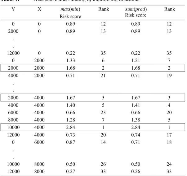
Now, the total study area (100 km2) is divided in to 2 km × 2 km grids. The 3-tuple fuzzy sets for exposure and hazard parameters at 35 locations in the studied area are composed as 5-tuple fuzzy sets of risk (see Table 8). Two compositional rules - max(min) and sum(prod) - are employed for this composition.

The 5-tuple fuzzy risk is later converted into crisp risk score (by defuzzification) using Equation 8. The higher value of a risk score (R) refers to a high priority for that location to be monitored. Figure 5 depicts the distribution of risk score over the area under study. The highest risk score (2.84) was obtained at location X = 10,000 and Y = 4,000 using both compositional methods. The second important location is X = 2000 and Y = 2000, where the risk sore is as high as 1.68. The results of the risk score and the corresponding ranking order of 35 locations are summarized in Table 9 for both max(min) and sum(prod) compositional rule. It is evident from the Table 9 that five locations are exceeding risk score to more than

1.38. The study suggests monitoring of first five main regions (ranked 1 to 5). This

monitoring location differs with the current monitoring locations, which are designed based on population.

In the aggregation/composition of exposure and hazard parameters, recognition of two potential pitfalls, namely exaggeration and eclipsing, is important. Exaggeration occurs when all parameters are of relatively low risk, yet the final risk comes out unacceptably high. Eclipsing is the opposite phenomenon, where one or more of the parameters is of relatively high risk, yet the estimated risk comes out as unacceptably low. These phenomena are typically affected by the aggregation method used, thus the challenge is to determine the best aggregation method which will simultaneously reduce both exaggeration and eclipsing.

Aggregation operators used for the development of environmental indices generally include additive forms (simple addition, arithmetic average, weighted average), root sum power, root sum square, maximum, multiplicative forms (e.g., geometric mean, weighted product), and minimum operators (Silvert, 2000; Somlikova and Wachowiak, 2001; Ott, 1978).

Model predictions may be sensitive to both the types of aggregation operators as well as to weights. Generally, a sensitivity analysis is conducted to quantify the change in output caused by changes in input values. In the proposed framework the sensitivity analysis should be

extended to examine the effects of weights and aggregation operators as well. A comprehensive sensitivity analysis will depend on the actual values of the specific case at hand. As the case study presented here is a simplified example, applying such a sensitivity analysis here would be of little value.

The proposed methodology has several advantages:

It enables the synthesis of quantitative information into qualitative output which is more easily understandable to decision makers and regulators;

It can explicitly consider and propagate uncertainties;

Its modular form is scalable; enabling it to easily accommodate new hazard and exposure parameters;

It is easily programmable for computer applications and can become a risk analysis tool for air quality monitoring;

The major limitation of the proposed method is that it may be sensitive to the selection of aggregation operators. Different operators can be used for different segments of the model. Trial and error approach may be required to avoid exaggeration and eclipsing. The application

presented in this paper is a simplified demonstration of the approach. A comprehensive application would require a major effort, including the collaboration of several experts in the various disciplines of knowledge. Works towards this end is in progress.

6. SUMMARY AND CONCLUSIONS

Air quality is affected by various sources of pollution. Quantification and characterization of the various exposure and hazard parameters is a complex process. The range of air pollutants, vulnerability of environmental conditions, increasing population and lack of understanding of some factors and processes affecting human health make it further challenging. Air quality monitoring over a wide area is a challenging activity, as it requires large resources. Traditionally, air quality monitoring networks are designed based on either concentration level of pollutants (hazard) or the sensitivity of receptor (exposure). Both approaches only capture the partial picture of the real world where actual damage is related to both factors - hazard and exposure. Having obvious importance, very little work on risk-based air quality monitoring is reported in the literature. Here we introduced a risk-based approach that tries to overcome this deficiency by encompassing these factors for risk quantification, which may guide us to better

decision-making.

In this study, an approach is developed to rank or prioritize air pollution monitoring locations based on the concept of risk. Risk is defined as a product of hazard and its likelihood of exposure, where both factors are expressed in terms of quantitative scales (defined by 3-tuple fuzzy sets). A modular hierarchical model is developed to provide a framework for aggregating hazard and exposure parameters. An analytic hierarchy process is used for the aggregation of hazard and exposure parameters. Two fuzzy compositional rules – sum(prod) and max(min) are used to determine a 5-tuple fuzzy set for risk. Further research is required to develop an elaborate

system, including expert panels and processes for the selection of the most appropriate operators and compositional method.

In the model development stages, the risk value is expected to have limited meaning for the acceptability of risk by the public. It is envisaged that as this methodology is developed, populated and subsequently improved upon (using newly obtained data), the developers will gain insight into acceptable risk levels as they are manifested in the final fuzzy and/or defuzzified risk values. In the longer terms, this approach could serve as a basis for bench marking acceptable risks in air pollution monitoring.

7. REFERENCES

Bates, D.V. 1992. Health indices of the adverse effects of air pollution: the question of coherence, Environmental Research, 59: 336 –349.

Baldauf, R.W., Lane, D.D., Marotz, G.A., Barkman, H.W., Pierce, T. 2002. Application of a risk assessment based approach to designing ambient air quality monitoring networks for

revaluating non-cancer health impacts, Environmental Monitoring and Assessment, 78: 213-227.

Baldauf, R.W., Lane, D.D., Marotz, G.A. 2001. Ambient air quality monitoring network design for assessing human health impacts from exposure to air borne contaminants, Environmental

Monitoring and Assessment, 66: 63-76.

Bonissone, P.P. 1997. Soft computing: the convergence of emerging reasoning technologies, Soft

Computing, 1: 6-18.

Burnett, R.T., Dales, R.E., Brook, J.R.,Raizenne, M.E.,Krewski, D. 1997.Association between ambient carbon monoxide levels and hospitalization for congestive heart failure in the elderly in 10 Canadian cities, Epidemiology 8: 162 –167.

Chen, S.J., and Hwang, C.L. 1992. Fuzzy multiple attribute decision-making, Springer-Verlag, NY.

Cheng, C-H, and Lin, Y. 2002. Evaluating the best main battle tank using fuzzy decision theory with linguistic criteria evaluation, European Journal of Operation Research, 142:174-186. Goldberg, A.S., Burnett, R.T., Valois, M.F., Flegel, K., Bailer III, J.C., Brook, J., Vincent, R.,

Radon, K. 2003. Association between ambient air pollution and daily mortality among persons with congestive heart failure, Environmental Research, 91: 8-20.

Harrison, R.M. and Deacon A.R. 1998. Spatial correlation of automatic air quality monitoring at urban background sites: implications for network design, Environmental Technology 19:121– 132.

Khan, F.I., Sadiq, R., and Husain, T. 2002. GreenPro-I: A risk-based life cycle assessment and decision-making methodology for process plant design, Environmental Modelling and

Software, 17: 669-692.

Kwon,H.-J.,Cho,S.-H.,Nyberg,P.,Pershagen,G. 2001. Effects of ambient air pollution on daily mortality in a cohort of patients with congestive heart failure, Epidemiology, 12: 413–419. Klir, G.J., and Yuan, B. 1995. Fuzzy sets and fuzzy logic - theory and applications, Prentice-

Hall, Inc., Englewood Cliffs, NJ, USA.

Lascio, L.D., Gisolfi, A., Albunia, A., Galardi, G., and Moschi, F. 2002. A fuzzy-based methodology for the analysis of diabetic neuropathy, Fuzzy Sets and Systems, 129: 203-228. Lowrence, W.W. 1976. Of acceptable risk, William Kaufmann, Los Altos, CA.

Lawry, J. 2001. A methodology for computing with words, International Journal of Approximate

Reasoning, 28: 51-89.

Lee, C.C. 1990a. Fuzzy logic in control systems: fuzzy logic controller – I, IEEE Transactions

on Systems, Man and Cybernetics, 20(2): 404-418.

Lee, C.C. 1990b. Fuzzy logic in control systems: fuzzy logic controller – II, IEEE Transactions

on Systems, Man and Cybernetics, 20(2): 419-435.

Lee, H.-M. 1996. Applying fuzzy set theory to evaluate the rate of aggregative risk in software development, Fuzzy Sets and Systems, 79: 323-336.

Lu, R-.S., and Hu, J-.Y. 1999. Analysis of reservoir water quality using fuzzy synthetic evaluation, Stochastic Environmental Research and Risk Assessment, 13: 327-336.

Lu, R.-S., and Lo, S.-L. 2002. Diagnosing reservoir water quality using self-organizing maps and fuzzy theory, Water Research, 36: 2265-2274.

Ott, W.R. 1978. Environmental indices: theory and practice, Ann Arbor Science Publishers Inc., pp. 371.

Morris,R.D.,Naumova,E.N.,1998.Carbon monoxide and hospital admissions for congestive heart failure: evidence of an increased effect at low temperatures. Environment Health Perspective, 106:649 –653.

Ricci, P.F., Sagen, L.A., and Whipple, C.G. 1981. Technological risk assessment series E: Applied Series No.81.

Rowe, N. 1977. Risk: an anatomy of risk, John Wiley and Sons, NY.

Saaty, T.L. 1988. Multicriteria decision-making: the analytic hierarchy process, University of Pittsburgh, Pittsburgh, Pa, USA.

Sadiq, R., and Rodriguez, M.J. 2004. Fuzzy synthetic evaluation of disinfection by-products – a risk-based indexing system, Submitted to Journal of Environmental Management.

Sadiq, R., Kleiner, Y., and Rajani, B.B. 2004a. Aggregative risk analysis for water quality failure in distribution networks, Aqua -Journal of Water Supply: Research and Technology (in press). Sadiq, R., Rajani, B., and Kleiner, Y. 2004b. A fuzzy-based method to evaluate soil corrosivity

for prediction of water main deterioration, ASCE, Journal of Infrastructure Systems (in press). Seaton, A., MacNee, W., Donaldson, K., Godden, D.1995. Particulate air pollution and acute health effect, Lancet, 345: 176 –178.

Silvert, W. 2000. Fuzzy indices of environmental conditions, Ecological Modelling, 130(1-3): 111-119.

Somlikova, R., and Wachowiak, M.P. 2001. Aggregation operators for selection problems, Fuzzy

Sets and Systems, 131: 23-34.

United States Environmental Protection Agency (US EPA). 1998. Revised draft user’s guide for

the AMS/EPA regulatory model (AERMOD). Pacific Environmental Services Inc., Research Triangle Park, North Carolina, p324, USA.

Yager, R.R. 1980. A general class of fuzzy connectives, Fuzzy Sets and Systems, 4: 235-242. Zadeh, L.A. 1996. Fuzzy logic computing with words, IEEE Transactions – Fuzzy Systems, 4(2):

Table 1. Adverse health and environmental effects.

Health hazard air pollution parameters

Adverse health and environmental effects

CO Cardiovascular effects: Low level CO is most serious for those who suffer from heart

disease, like angina, clogged arteries, or congestive heart failure.

Central Nervous System effects: High levels of CO can develop vision problems, reduced ability to work or learn, reduced manual dexterity, and difficulty performing complex tasks.

Poisonous: At extremely high levels, CO is poisonous and can cause death. Smog: CO contributes to the formation of smog ground-level ozone, which can trigger serious respiratory problems.

NOx Smog: involved in the formation of ground-level ozone, which can trigger serious

respiratory problems. Acid rain

Nutrient overload deteriorates water quality.

Visibility impairment: reacts with atmospheric particles. Formation of toxic chemicals.

Global warming

PM10 Health effects

aggravated asthma

coughing and difficult or painful breathing chronic bronchitis

decreased lung function premature death Visibility impairment Atmospheric deposition

acidic lakes and streams

imbalance of nutrient level on coastal waters and large river basins. depleting of nutrients in soil

damaging sensitive forests and farm crops affecting the diversity of ecosystems Aesthetic damage

soot stains and damages materials, including culturally important objects such as monuments and statues.

SOx Respiratory effects from gaseous SO2 and Sulfates

Visibility impairment Acid rain

Plant, soil and water damage Forests and crops

Table 2. Ambient air quality guidelines (µg/m3) for 24-hour average

Health hazard air pollution parameters Newfoundland -Labrador Canada US EPA CO *15,700 *10, 000 (P) NOx 200 100 (P, S) PM10 50-60 **120 150 (P, S) SOx 300 365 (P,S) * 8-hour average

** total suspended particulates (acceptable level) P: primary standards and S: secondary standards

Table 3. Health hazard air pollution parameters - membership functions

Hazard air pollution parameters Applicability of range (µg/m3) Membership to Low Membership to Medium Membership to High CO x ≤ 10,000 1 0 0 10,000 <x ≤ 15,000     ₋ − 000 5 000 10 1 , , x     − 000 5 000 10 , , x 0 15,000 <x ≤ 20,000 0     ₋ − 000 5 000 15 1 , , x     − 000 5 000 15 , , x x > 20,000 0 0 1 NOx x ≤ 150 1 0 0 150 <x ≤ 200     ₋ − 50 150 1 x _ − _ 50 150 x 0 200 <x ≤ 250 0     ₋ − 50 200 1 x _ − _ 50 200 x x > 250 0 0 1 PM10 x ≤ 40 1 0 0 40 <x ≤ 60     ₋ − 20 40 1 x _ − _ 20 40 x 0 60 <x ≤ 80 0     ₋ − 20 60 1 x _ − _ 20 60 x x > 80 0 0 1 SOx x ≤ 200 1 0 0 200 <x ≤ 300     ₋ − 100 200 1 x _ − _ 100 200 x 0 300 <x ≤ 400 0     ₋ − 100 300 1 x _ − _ 100 300 x x > 400 0 0 1

Table 4. Definitions for exposure parameters

Exposure parameters Scale

Location sensitivity (LS) – Available amenities

No-basic facility 0

Facilities of low value (e.g., storage facilities) 2 Factories and industry 4

Residential, parks 6

Schools, churches, heritage places 8 Hospitals, sensitive locations 10

Population density (PD) – Number of people/area

<20 1

20-49 2

50-99 3

100-300 4

>300 5

Population sensitivity (PS) – Percent sensitive population

< 10 1

10-25 2

26-40 3

41-50 4

Table 5. Exposure parameters - membership functions membership functions

Exposure criteria

Applicability of range Membership to

Low Membership to Medium Membership to High LS x ≤ 4 1 0 0 4 <x ≤ 6     ₋ − 2 4 1 x _ − _ 2 4 x 0 6 <x ≤ 8 0     ₋ − 2 6 1 x _ − _ 2 6 x x > 8 0 0 1 PD x ≤ 2 1 0 0 2 <x ≤ 3     ₋ − 1 2 1 x _ − _ 1 2 x 0 3 <x ≤ 4 0     ₋ − 1 3 1 x _ − _ 1 3 x x > 4 0 0 1 PS x ≤ 2 1 0 0 2 <x ≤ 3     ₋ − 1 2 1 x _ − _ 1 2 x 0 3 <x ≤ 4 0     ₋ − 1 3 1 x _ − _ 1 3 x x > 4 0 0 1

Table 6. Fundamental scale used to developing priority matrix for AHP (Saaty, 1988)

Intensity of

importance Definition Explanation

1 Equal importance Two activities contribute equally to the objective

2 Weak -

3 Moderate importance Experience and judgement slightly favour one activity over other

4 Moderate plus -

5 Strong importance Experience and judgement strongly favour one activity over other

6 Strong plus -

7 Very strong or

demonstrated importance

An activity is favoured very strongly over another; its dominance demonstrated in practice 8 Very, very strong -

9 Extreme importance The evidence favouring one activity over another is of highest possible order of affirmation

Table 7. Weights for hazard and exposure parameters Weights Values wCO 0.14 wNOx 0.22 wPM10 0.28 wSOx 0.36 wLS 0.13 wPD 0.21 wPS 0.66

Table 8. Risk matrix for rule-base

Exposure

Hazard Low Medium High

Low Very low Low Medium

Medium Low Medium High

Table 9. Risk score and ranking of monitoring locations Y X max(min) Risk score Rank sum(prod) Risk score Rank 0 0 0.89 12 0.89 12 2000 0 0.89 13 0.89 13 . . 12000 0 0.22 35 0.22 35 0 2000 1.33 6 1.21 7 2000 2000 1.68 2 1.68 2 4000 2000 0.71 21 0.71 19 . . 2000 4000 1.67 3 1.67 3 4000 4000 1.40 5 1.41 4 6000 4000 0.66 23 0.66 20 8000 4000 1.28 7 1.38 5 10000 4000 2.84 1 2.84 1 12000 4000 0.73 20 0.74 17 0 6000 0.87 14 0.71 18 . . 10000 8000 0.50 26 0.50 24 12000 8000 0.27 33 0.26 33

Scoring method

Fuzzification

Defining qualitative scales (low, medium, high) Mapping observed values on these scales

3-tuple fuzzy sets for each hazard parameter

CO, NOx, SOx, and PM10

3-tuple fuzzy sets for each exposure parameter

Location sensitivity, Population sensitivity and density

Cumulative hazard -tuple fuzzy set 3

Cumulative exposure 3-tuple fuzzy set

Fuzzy rule-base 5-tuple fuzzy risk

Defuzzification

Defuzzification methods include first of maximum, mean of maximum, last of maximum and centre of area, scoring method, etc.

Prioritization of monitoring locations based on risk Composition of hazard and

exposure fuzzy sets e.g. max(min), sum (prod) Analytic Hierarchy Process (AHP)

Estimating weights for exposure and hazard parameters

Trapezoidal fuzzy number

Triangular fuzzy number

Identification of hazard and exposure parameters

Hazard: Concentration of CO, NOx, SOx, and PM10

Exposure: Location sensitivity, Population density and sensitivity

Aggregation

[

]

[

]

0.00 2000.00 4000.00 6000.00 8000.00 0.00 2000.00 4000.00 6000.00 8000.00 10000.00 12000.00 Receptors (comunities) Stacks 10000 12000 14000 16000 18000 20000 22000 24000 26000 28000 30000 32000 a) CO 0.00 2000.00 4000.00 6000.00 8000.00 0.00 2000.00 4000.00 6000.00 8000.00 10000.00 12000.00 Receptors (communities) Stack 140 160 180 200 220 240 260 280 300 320 340 360 380 400 420 440 460 480 b) NOx 0 1000 2000 3000 4000 5000 6000 7000 8000 0 1000 2000 3000 4000 5000 6000 7000 8000 9000 10000 11000 12000 Recetors (communities) Stack 50 60 70 80 90 100 110 120 130 140 c) PM10 0.0 2000.0 4000.0 6000.0 8000.0 lateral distance, m 0.0 2000.0 4000.0 6000.0 8000.0 10000.0 12000.0 ve rt ical dist a n ce, m Receptors (comunity) Stacks 200 250 300 350 400 450 500 550 600 650 700 750 800 850 d) SOx Figure 3. Distribution of health hazard air pollution parameters

0.00 2000.00 4000.00 6000.00 8000.00 0.00 2000.00 4000.00 6000.00 8000.00 10000.00 12000.00 Receptors (comunities) Stacks 1 2 3 4 5 6 7 8 9 a) LS 0.00 2000.00 4000.00 6000.00 8000.00 0.00 2000.00 4000.00 6000.00 8000.00 10000.00 12000.00 Receptors (comunities) Stacks 1 2 2 3 3 4 4 5 5 6 b) PD 0.00 2000.00 4000.00 6000.00 8000.00 0.00 2000.00 4000.00 6000.00 8000.00 10000.00 12000.00 Receptors (comunities) Stacks 1.0 1.5 2.0 2.5 3.0 3.5 4.0 4.5 c) PS

0 1000 2000 3000 4000 5000 6000 7000 8000 0 500 1000 1500 2000 2500 3000 3500 4000 4500 5000 5500 6000 6500 7000 7500 8000 8500 9000 9500 10000 10500 11000 11500 12000 Residential communities Stacks 0.80 1.00 1.20 1.40 1.60 1.80 2.00 2.20 2.40 2.60