Shallow water wave correction in the OEB (multichromatic waves)

(1)

Publisher’s version / Version de l'éditeur:

Vous avez des questions? Nous pouvons vous aider. Pour communiquer directement avec un auteur, consultez la

première page de la revue dans laquelle son article a été publié afin de trouver ses coordonnées. Si vous n’arrivez

Questions? Contact the NRC Publications Archive team at

[email protected]. If you wish to email the authors directly, please see the first page of the publication for their contact information.

https://publications-cnrc.canada.ca/fra/droits

L’accès à ce site Web et l’utilisation de son contenu sont assujettis aux conditions présentées dans le site LISEZ CES CONDITIONS ATTENTIVEMENT AVANT D’UTILISER CE SITE WEB.

Technical Report; no. TR-2011-05, 2011-03

READ THESE TERMS AND CONDITIONS CAREFULLY BEFORE USING THIS WEBSITE. https://nrc-publications.canada.ca/eng/copyright

NRC Publications Archive Record / Notice des Archives des publications du CNRC :

https://nrc-publications.canada.ca/eng/view/object/?id=89de36f6-e710-4c67-a46c-1fcb63198598 https://publications-cnrc.canada.ca/fra/voir/objet/?id=89de36f6-e710-4c67-a46c-1fcb63198598

NRC Publications Archive

Archives des publications du CNRC

For the publisher’s version, please access the DOI link below./ Pour consulter la version de l’éditeur, utilisez le lien DOI ci-dessous.

https://doi.org/10.4224/19541695

Access and use of this website and the material on it are subject to the Terms and Conditions set forth at

Shallow water wave correction in the OEB (multichromatic waves)

(2)

DOCUMENTATION PAGE

REPORT NUMBER

TR-2011-05

NRC REPORT NUMBER DATE

March 2011 REPORT SECURITY CLASSIFICATION

Unclassified

DISTRIBUTION

Unlimited TITLE

SHALLOW WATER WAVE CORRECTION IN THE OEB (MULTICHROMATIC WAVES) AUTHOR (S)

Hasanat Zaman1, Heather Peng2, Emile Baddour1 and Shane McKay1 CORPORATE AUTHOR (S)/PERFORMING AGENCY (S)

1

Institute for Ocean Technology, National Research Council, St. John’s, NL 2

Memorial University of Newfoundland PUBLICATION

SPONSORING AGENCY(S)

IOT PROJECT NUMBER 42_2414_26

NRC FILE NUMBER

KEY WORDS

JONSWAP, TMA spectrums, second order spurious waves, code (LWAVE)

PAGES iii, 193, App. I-III FIGS. 199 (App.) TABLES 4 SUMMARY

Accurate generation of the primary waves and the reproduction of the group-induced second-order low and high frequency waves have been considered essential for physical model test in the laboratory. In the laboratory when multi-chromatic primary waves are generated the required bounded waves will be generated naturally at the difference frequencies. In addition to that several unwanted free waves are also generated. The free waves, having the same frequencies of the bounded waves are reproduced due to mismatch of the boundary conditions at the wave paddle. The other two types of free waves are due to the wave paddle displacement and the local disturbances. We carried out physical experiments to identify the second order spurious waves in shallow water in the Offshore Engineering Basin (OEB) at the Institute for Ocean Technology (IOT) of National Research Council (NRC) Canada. In the basin water depths in the range of 0.4m to 0.6m are used for the experiments. The peak wave periods also have varied from 1.133s to 2.145s. In this experiment JONSWAP and TMA spectrums are separately used. The drive signals of the wave-makers are generated using first-order and second-order wave generation techniques. Total 14 wave probes are used to capture the data in the wave tank. A NRC-IOT code (LWAVE) is used to isolate the primary waves, the bounded waves and the unwanted free waves from the measured data at each wave probe. The measured data are analyzed in this paper to illustrate the differences in the waves generated by two different generation techniques.

ADDRESS National Research Council Institute for Ocean Technology Arctic Avenue, P. O. Box 12093 St. John's, NL A1B 3T5

(3)

National Research Council Conseil national de recherches Canada Canada

Institute for Ocean Institut des technologies Technology océaniques

SHALLOW WATER WAVE CORRECTION IN THE OEB

(Multichromatic waves)

TR-2011-05

Hasanat Zaman, Heather Peng, Emile Baddour and Shane McKay March 2011

(4)

TABLE OF CONTENTS 1.0 INTRODUCTION ... 1 2.0 THEORY ... 2 3.0 EXPERIMENTS ... 5 3.1 Software ... 5 3.2 Experimental setup... 5

4.0 CASE STUDY: Multi-chromatic waves ... 8

4.1 A typical comparison ... 8

4.2 Comparisons of the wave generation techniques using JONSWAP spectrum ... 9

4.3 Comparisons of the first-order waves using JONSWAP and TMA spectrums 10 5.0 METHODOLOGY ... 11

6.0 RESULTS ... 11

7.0 CONCLUSIONS ... 11

8.0 ACKNOWLEDGEMENT... 12

9.0 REFERENCES... 12

Appendix I Comparisons of the first- and second-order wave spectrums for all water depths (0.4m, 0.5m and 0.6m). JONSWAP spectrum is used as input Appendix II Isolated wave components obtained from both first- and second-order measured wave profiles using Lwave computer codes. Appendix III Comparisons of the first- and second-order wave spectrums for all water depths (0.4m, 0.5m and 0.6m). JONSWAP and TMA spectrums are used as inputs. LIST OF PHOTOS Photo 1: Setup of 14 wave probes in the OEB. Photo 2: 8 wave probes are set over the cross LIST OF TABLES Table 1: Location of the wave probes in the OEB... 7

Table 2: Incident wave parameters ... 8

Table 3: Comparisons of Free waves and Bounded waves... 9

(5)

ABSTRACT

Accurate generation of the primary waves and the reproduction of the group-induced second-order low and high frequency waves have been considered essential for physical i.e. model test in the laboratory. In the laboratory when multi-chromatic primary waves are generated the required bounded waves will be generated naturally at the difference frequencies. In addition to that several unwanted free waves are also generated. The free waves, having the same frequencies of the bounded waves are reproduced due to mismatch of the boundary conditions at the wave paddle. The other two types of free waves are due to the wave paddle displacement and the local disturbances.

We carried out physical experiments to identify the second order spurious waves in shallow water in the Offshore Engineering Basin (OEB) at the Institute for Ocean Technology (IOT) of National Research Council (NRC) Canada. In the basin water depths in the range of 0.4m to 0.6m are used for the experiments. The peak wave periods also have varied from 1.133s to 2.145s. In the experiments multi-chromatic waves are used. The drive signals of the wave-makers are generated using first-order and second-order wave generation techniques. Total 14 wave probes are used to capture the data in the wave tank. A NRC-IOT code is used to isolate the primary waves, the bounded waves and the unwanted free waves from the measured data at each wave probe. The measured data are analyzed in this paper to illustrate the differences in the waves generated by two different generation techniques. Both JONSWAP and TMA spectrums are used in the experiments.

1.0 INTRODUCTION

During the generation of multi-chromatic primary waves in the wave basin the required bounded waves will also be generated naturally at the difference frequencies. On top of that several unwanted free waves are also generated. The second order free wave FW-1, having the same frequency of the bounded wave is reproduced due to mismatch of the boundary conditions at the wave paddle. The second order free wave FW-2 appears due to the displacement of the wave paddle. The second order free wave FW-3 is due to the local disturbances. The local disturbances usually disappear at some distance from the wave-makers and thus will not be discussed here. If the wave basin is not unconditionally flat then there might be some other types of unwanted free waves in the basin in addition to the aforesaid three categories.

Proper understanding of the effects of the wave-action and consequent loading pattern of the primary waves along with their bounded waves are very important factors to design, implementation and operation of any ocean structures, mooring system, floating vessels, harbour resonance, etc..

In an accurate physical model test in the laboratory it is crucial to choose the precise design parameters of such structures and/or vessels, etc. So it is essential to reduce or eliminate the unwanted free waves components for physical model tests and to ensure the reproduction of the group-induced second-order low frequency and high frequency components in the laboratory. Please see Zaman and Mak (2007) for high frequency second-order wave components and Zaman et al (2010) for mono- and bi-chromatic waves, not to be discussed here.

In the case of multi-chromatic waves the simplest unit contributing to the second order waves is a two-frequency group. In such a wave field the total contributions of any

(6)

unwanted free waves is the summation of all the similar components due to interaction of any two wave components in the multi-frequency wave field. A two-frequency wave group is evolved due to the interaction of any two waves of frequencies f1 and f2, the

group-induced second-order low and high frequency waves are generated along with other unwanted free waves. A low frequency wave or bounded wave will be produced due to the difference (f1 – f2) of the frequencies and a high frequency or short wave would

be generated due to the summation (f1 + f2) of the frequencies. The profile of the bounded

wave having frequency (f1 – f2) is generally termed as the set-down in the larger wave

zone and the set-up in the smaller wave zone. These set-down and set-up phenomena were first investigated and reported by Longuet-Higgins and Stewart (1961, 1962, 1963, 1964 and 1977) in a series of papers. They introduced the radiation stress concept, which explained that in a wave group individual wave components exerted an internal compressive force in the direction of the wave propagation. To balance this force the mean water level goes down in the region of larger waves known as set-down and goes up in the region of smaller waves known as set-up. Bowen et al (1968) later explained the set-up and set-down phenomena with experimental data.

The theoretical and experimental descriptions of such natural high and low frequency waves along with their various unwanted free waves were given by many researchers. Hansen (1978), Sand (1982), Barthel et al (1983), Sand and Mansard (1986a, b), Mansard (1991), Mansard et al (1987), Schaffer (1993), Stansberg (2006), Zaman and Mak (2007), Zaman et al (2010), Spinneken and Swan (2009) are a few who described the methods to curtailing these unavoidable free waves from the resulting surface elevations in the wave basin.

In our present experiments the first-order wave generation (FOG) and the second-order wave generation (SOG) techniques for the multi-chromatic waves were used. JONSWAP spectrums are used to generate both first- and second-order waves in the OEB. In the experiment water depths are varied in the range of 0.4m to 0.6m. The wave periods also have varied from 1.133s to 2.145s. Comparisons are made between data obtained from the first-order wave generation technique and the second-order wave generation technique using JONSWAP spectrums as input. For the case of the first-order generation technique we compared experimental data obtained using both JONSWAP and TMA spectrums as inputs.

2.0 THEORY

A wave group would be generated with the presence of at least two frequencies. The difference of these two frequencies would generate a long period bounded wave with a period equal to the period of the wave group. This long wave is also known as ‘set-up and set-down’. The description of the waves in nature is normally given by a wave spectrum. For irregular waves with a given spectral density, by Fourier series expansion, the first order wave profile (see Sand 1982) can be written as function of the coefficients a and n

n b . ) sin( ) cos( ) , ( 1 1 x t a nt knx bn nt knx N n n    



    (1)

(7)

In which Nis the total number of frequencies in the wave trains, nis the cyclic frequency and k is the wave number, n a and n b are the Fourier coefficients, n respectively.

For the piston type wave maker, the first-order control signal is given by the summation of contributions from all the frequencies in the spectrum [see also (Barthel et al (1983) and Sand and Mansard (1986b)].

1 2 1 cosh( ) sinh( ) ( ) ( sin( ) cos( )) 2sinh ( ) N n n n n n n n n n k d k d k d X t a t b t k d        _  _  



(2)

The simplest unit contributing to the second order waves is a two frequency group. The total second order wave elevation is then found as the summation of the contributions from all pairs of frequencies.

By means of Laplace equations, the second order contributions due to one pair of difference frequency can be given as follows:

2( , ) ( ) cos( ) ( ) sin( ) mn m n m n mn mn mn m n n m mn mn x t G a a b b t k x G a b a b t k x                     (3)

where Gmn is a second order quadratic transfer function, mn n m

 and m n mn k k k    

, n and m are the index of one pair of difference frequency. The quadratic transfer function is given by the following equation:

( ) ( (1 tanh tanh ) 2 4 1 ( tanh tanh )) 4 nm n m m n mn m n m n m m n n A k k g G k d k d g k k d k k d        _  _ _ _  (4) where, 2 2 1 2 ( ) ( ) tanh( ) mn mn nm n m n m n m B C A g k k g k k d      _      2 2 2 2 cosh cosh m n mn m m n n k k B k d k d    _ _ 2 m n( n m)(1 tanh m tanh n ) mn m n k k k d k d C      _  

(8)

where, d is the water depth and g is the acceleration due to gravity and       m n m n 5 . 0 1 

The second order control signal for a correct reproduction of the wave train up to second order takes the following form:

0 0 2 1 23 1 23 ( ) (( ) ( ) ) cos( ) (( ) ( ) ) sin( ) N N n n m m n n m m n n f m f mn n m m n m n n m mn X t a b a b F a a b b F t a a b b F a b a b F t                        

 

(5)

The function, F₁ is written as:

   _ _ 12 11 1 F F F (6) 11 2 2 ( )sinh( ) / ( )sinh( ) 2(( ) ( ) )sinh( )sinh( ) mn f mn f mn f mn f mn f mn f mn f k d k d k d k d F G k d k d k d k d k d k d k d k d k d                 _     _     _ _        __ __            (7) 12 2 2 2 2 (1 )[ sinh( ) sinh( )]

8( )(( ) ( ) )sinh( )sinh( ) tanh( )

(1 )[ sinh( ) sinh( )] 8( )(( ) ( ) )sinh( )sinh m f m n m m m m n m m f f m n n f n m n n n n n m n f f f k k d H k d k d k d k d F f f k d k d k d k d k d f k k d H k d k d k d k d f f k d k d k d                                        (k d_n ) tanh(k d_m ) (8)

The free long wave number, k_f is computed from the dispersion relation given as:

2 (_mn )  g k_f tanh(k d_f ) (9) where, m m f k k k   _ _{ }   _ __  f n n k k k  ; 2 ; 2 sinh(2 ) sinh(2 ) m n m n m n k d k d H H k d k d   ) ( ₃_, ₃_, 2 23     _ _ n m F F F F (10)

(9)

2 (1 )(1 ) 8 tanh( ) tanh( ) f m n m n k H H F k d k d  _    (11) 2 n fn    (12) 2 m fm    (13) 3, 2 2 1

2 sin( )[ sin( )coth( ) cos( )]

( ) (( ) ( ) )(sin( )cos( ) ) j j j j f f j m m j n m j f j j j k d k d k d k d k d k d k d f F f f k d k d k d k d k d          



   (14)

where, k d is computed from the following expression: j

2 tan( ) m j j d k d k d g    ,with 1 2 (j ) k d_j  j (15)

In the above equation, fn and fm are the possible frequency components in the wave field.

For example, for only two waves the above frequency components will be modified to f1

and f2, respectively. The functions F11 

and F₁₂ respectively, will reduce or eliminate the Free wave-1 and Free wave-2 from the wave field. The function F₂₃ is to eliminate the second order free wave-3 due to local disturbances. This function is not considered here as the local disturbances disappear after some distance from the wave maker

3.0 EXPERIMENTS

The experiment was carried out at the Offshore Engineering Basin of National Research Council Canada, Institute for Ocean Technology. The top view of the basin is shown in Fig. 1. The Offshore Engineering Basin is 75 m long x 32 m wide. 56 independently controlled segmented wave generators installed on the west wall generated the waves. Each segmented wave generator is 2 m high and 0.5 m wide. Passive absorbers, made of expanded metal sheets with varying porosities and spacing, are installed on the east wall. A solid metal wall is used to cover the north side of the basin. The water depths for the experiments are 0.4m, 0.5m and 0.6m.

3.1 Software

In IOT bichromatic waves are generated using WAVE computer code. This is a first order wave generation code. The second order wave generation code is developed using Sand’s (1982) formulae. We used these two codes to generate waves in the OEB. When surface elevations are measured a computer code called LWAVE is used to isolate all component waves.

3.2 Experimental setup

During the experiment, 14 wave probes installed as shown in Fig. 1 and Table-1 measured the location of the wave probes throughout the basin. All the wave probes are capacitance type. All the data was acquired using GDAC (GEDAP Data Acquisition and Control) client-server acquisition system, developed by National Research Council

(10)

Canada, Institute for Ocean Technology. The bottom of the basin was flat and the blanking plates were deployed to cover the north beach.

Fig. 1: Top view of the experimental setup in the OEB

Photo 1: Setup of 14 wave probes in the OEB. P-11 P-7 P-1 P-2 P-3 P-6 P-4 P-5 P-14 P-9 P-10 P-8 P-12 P-13 13.475 Wave-makers 2m 10.744 South wall Beach

(11)

Photo 2: 8 wave probes are set over the cross

Table 1 Location of the wave probes in the OEB No of the

probe

Distance from the east wave paddle (m)

Distance from the south wall (m) 1 26.891 13.475 2 27.221 13.475 3 27.731 13.475 4 27.731 12.955 5 27.731 12.635 6 27.731 14.825 7 27.731 18.365 8 29.081 13.475 9 32.621 13.475 10 41.621 13.475 11 2.0 12.635 12 2.0 13.475 13 2.0 18.365 14 10.744 13.475

(12)

4.0 CASE STUDY: Multi-chromatic waves

In our present experiments the first-order and the second-order wave generation techniques for the multi-chromatic waves were used. We utilized JONSWAP and TMA spectrum systems for this experiment. In the experiment water depths are varied in the range of 0.4m to 0.6m. The wave periods also have varied from 1.133s to 2.45s.

Section 4.1 shows a typical comparison between the spectrums obtained from the first- and second-order wave generation techniques using JONSWAP condition. Comparisons of the obtained first- and second-order wave spectrums for JONSWAP condition are shown in details in section 4.2. On the other hand, comparisons of the first-order wave spectrums due to JONSWAP and TMA conditions are shown in section 4.3.

4.1 A typical comparison

In this typical comparison two cases of the 0.4m water depth experiments are used. Table 2 summarizes the incident wave parameters of the wave conditions examined in this paper.

Table 2 Incident wave parameters d (m) Tp (s) Hs (m) h/L

Case-1 0.4 1.133 0.06 0.224 Case-2 0.4 1.705 0.06 0.130

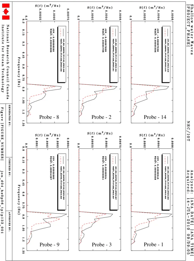
For each case, there were two runs, one used first-order generation technique and the other one used the second-order wave generation technique. Fig. 2 shows the comparisons of the spectrums at 6 different locations in the wave basin between first-order and second-first-order wave generation techniques for Case-1. These 6 locations are at Probe-14, Probe-1, Probe-2, Probe-3, Probe-8 and Probe-9. These probes are on the same line, see Fig. 1. In Fig. 2 it may be observed that the low frequency components are not prominent in either generation technique.

Fig. 3 shows the same comparisons for Case-2. In Fig. 3 one can perceive the differences in low frequency second order wave components between two different generation techniques. So from now on we will concentrate on Case-2 only to identify the spurious components. A NRC-IOT computer code that can split a surface elevation data set into its component waves is used to isolate the primary waves, bounded second order waves and unwanted free waves from the raw measured data at every probe location.

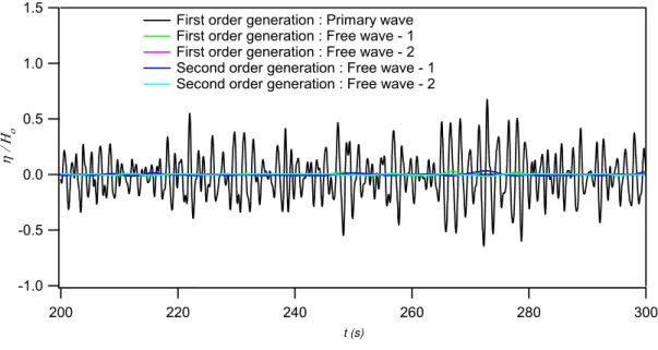
Figs. 4a and 4b show comparisons of various separated wave components for Case-2 at Probe-1. Fig. 4a shows the comparisons of the measured primary waves of first order generation with unwanted free waves of first order generation and second order generation techniques. Fig. 4b, on the other hand, shows the comparisons of the primary wave with bounded waves of first and second order generation techniques at Probe-1. Figs. 5a and 5b show similar comparisons at Probe-2 for Case-2.

From Figs. 4a and 5a it may be observed that the unwanted free waves obtained from both generation techniques are not significantly large with respect to their primary wave components.

Table 3 shows the comparisons of the bounded waves and unwanted free waves at two probe locations for both first-order and second-order generation techniques. The

(13)

comparisons [%= (FW1 / PW)*100] or [%= (FW2 / PW)*100] are done with respect to the measured significant primary wave height, PW = 0.0446m at Probe-1 and PW = 0.0496m at Probe-2 obtained in the first-order wave generation method, respectively.

Table 3 Comparisons of Free waves and Bounded waves FW1 (FOG) % FW1 (SOG) % FW2 (FOG) % FW2 (SOG) % BW (FOG) % BW (SOG) % Maximum wave heights

P-1 4.03 4.08 1.85 1.49 4.93 4.66

P-2 3.63 3.97 1.17 1.59 4.47 4.30

Average wave heights

P-1 1.65 1.55 0.88 0.75 2.14 2.08

P-2 2.03 1.93 1.03 0.88 2.62 2.12

Significant wave heights

P-1 3.01 2.71 1.51 1.13 4.02 3.30

P-2 3.37 3.32 1.63 1.29 4.18 3.44

P-1: Probe-1 and P-2 : Probe-2

FW1: Free wave-1, FW2: Free wave-2 and BW: Bounded wave

4.2 Comparisons of the wave generation techniques using JONSWAP spectrum

In this experiment three different types of water depths are used. Table 4 shows the wave conditions for all three water depths. For all water depths first order and second order wave generation techniques are utilized. Table 4 is used for both generation techniques. Comparisons of the wave spectrums obtained from two different wave generation techniques are shown. See Appendix-I for figures.

Figs. 6a,b, 7a,b and 8a,b show the comparisons of the wave spectrums for C4-1, C4-2 and C4-3 cases at Probe-14, Probe-1, Probe-2, Probe-3, Probe-8 and Probe-9. On the other hand, Figs. 6c,d,e,f, 7c,d,e,f and 8c,d,e,f show the obtained instantaneous surface elevations at different wave probe locations for both generation techniques.

Similarly Figs. 9a,b, 10a,b and 11a,b show the comparisons of the wave spectrums for C5-1, C5-2 and C5-3 cases at Probe-14, Probe-1, Probe-2, Probe-3, Probe-8 and Probe-9. Again, Figs. 9c,d,e,f, 10c,d,e,f and 11c,d,e,f illustrate the obtained instantaneous surface elevations at different wave probe locations for both generation techniques.

In the same fashion Figs. 12a,b, 13a,b and 14a,b show the comparisons of the wave spectrums for C6-1, C6-2 and C6-3 cases at 14, 1, 2, 3, Probe-8 and Probe-9. In the same way Figs. 12c,d,e,f, 13c,d,e,f and 14c,d,e,f demonstrate the obtained instantaneous surface elevations at different wave probe locations for both generation techniques.

(14)

Table 4 Incident wave parameters for three depths Tp (s) Hs (m) d(m) d/L C4-1 1.133 0.06 0.4 0.22 C4-2 1.705 0.06 0.4 0.13 C4-3 2.145 0.06 0.4 0.10 C5-1 1.133 0.06 0.5 0.27 C5-2 1.705 0.06 0.5 0.15 C5-3 2.145 0.06 0.5 0.11 C6-1 1.133 0.06 0.6 0.31 C6-2 1.705 0.06 0.6 0.17 C6-3 2.145 0.06 0.6 0.12

Appendix-II shows the isolated wave components of the required primary and the bounded waves and the unwanted free wave-1 due to mismatch of the boundary condition at the wave pedal and the unwanted free wave-2 for the movement of the wave pedal from its zero position. These isolated components are shown for C4-1, C4-2 and C4-3 cases only. As said before LWAVE code is used to isolate the component waves.

Figs. 15 a,b, 16a,b, 17a,b, 18a,b, 19a,b and 20a,b show the isolated wave components for both first- and second-order wave generation techniques respectively, at Probe-14, Probe-1, Probe-2, Probe-3, Probe-8 and Probe-9 for case C4-1. Similar components are shown in Figs. 21 a,b, 22a,b, 23a,b, 24a,b, 25a,b and 26a,b for case C4-2 and in Figs. 27a,b, 28a,b, 29a,b, 30a,b, 31a,b and 32a,b for case C4-3.

Figs. 33a,b, 34a,b, 35a,b, 36a,b, 36a,b and 38a,b show the isolated wave components for both first- and second-order wave generation techniques, at 14, 1, Probe-2, Probe-3, Probe-8 and Probe-9 for case C5-1. Similar components are shown in Figs. 39 a,b, 40a,b, 41a,b, 42a,b, 43a,b and 44a,b for case C5-2 and in Figs. 45a,b, 46a,b, 47a,b, 48a,b, 49a,b and 50a,b for case C5-3.

Figs. 51 a,b, 52a,b, 53a,b, 54a,b, 55a,b and 56a,b show the isolated wave components for both first- and second-order wave generation techniques, at 14, 1, Probe-2, Probe-3, Probe-8 and Probe-9 for case C5-1. Similar components are shown in Figs. 57 a,b, 58a,b, 59a,b, 60a,b, 61a,b and 62a,b for case C5-2 and in Figs. 63a,b, 64a,b, 65a,b, 66a,b, 67a,b and 68a,b for case C5-3.

4.3 Comparisons of the first-order waves using JONSWAP and TMA spectrums

In this experiment both JONSWAP and TMA spectrums are used to generate first-order waves. In this case also Table 4 shows the wave conditions that we used for both JONSWAP and TMA spectrums methods. Table 4 is used for both spectrum methods. Comparisons of the wave spectrums obtained from these two methods are shown.

Figs. 69a,b, 70a,b and 71a,b show the comparisons of the JONSWAP and TMA wave spectrums for C4-1, C4-2 and C4-3 cases at 14, 1, 2, 3, Probe-8 and Probe-9. On the other hand, Figs. 69c,d, 70c,d and 71c,d, show the obtained

(15)

instantaneous surface elevations at above wave probe locations for TMA spectrum condition.

Figs. 72a,b, 73a,b and 74a,b show the comparisons of the JONSWAP and TMA wave spectrums for cases C5-1, C5-2 and C5-3 at the above same locations and Figs. 72c,d, 73c,d and 74c,d, show the obtained instantaneous surface elevations at above wave probe locations for TMA spectrum condition.

Figs. 75a,b, 76a,b and 77a,b show the comparisons of the JONSWAP and TMA wave spectrums for cases C6-1, C6-2 and C6-3 at the above same locations and Figs. 75c,d, 76c,d and 77c,d, show the instantaneous surface elevations at above wave probe locations for TMA spectrum condition. See Appendix-III for figures.

5.0 METHODOLOGY

The FORTRAN code WAVE is used to generate eta-file for a given set of wave parameters (peak wave periods and significant wave heights). Another FORTRAN code DWREP2 will produce necessary drive signal from the above eta-file to generate the multi-chromatic waves in the OEB. This is we call first-order-generation technique. On the other hand, from the given set of wave parameters, a FORTRAN code SOG (not in GEDAP) will predict primary and bounded waves’ profiles that later transformed into drive signal using another FORTRAN code CONVERT and then generate multi-chromatic waves in the OEB.

6.0 RESULTS

In this experiment 3 different water depths (d= 0.4m, 0.5m and 0.6m) were used. However results of 3 different depths (d=0.4m, 0.5m and 0.6m) are shown and described here. The incident wave parameters are shown in Table- 4 for all three water depths that are used here. In this experiment relative water depths (d/L) were varied from shallow to intermediate water depth limits.

Both First-Order and Second-Order wave generation techniques were employed in the present experiments.

APPENDIX-I : Comparisons of first- and second-order spectrums for JONSWAP case. APPENDIX-II : Isolation of component waves using LWAVE for all depths.

APPENDIX-III : Comparisons of First-order waves in JONSWAP and TMA spectrums.

7.0 CONCLUSIONS

For the case of multi-chromatic wave generation, first-order and second-order wave generation techniques are used to study the propagation of the primary waves, bounded waves and unwanted free waves in the Offshore Engineering Basin of NRC-IOT. A typical comparison of the wave profiles and wave heights for Case-2 are shown. It is observed that the unwanted low frequency free wave components are not significant compare to the primary wave components. See Figs. 4a to 5b. Comparing first-order and second-order wave generation techniques, it is observed that the magnitudes of the unwanted free waves are very similar in both generation techniques. Details results for both generation techniques with different wave periods and water depths (d=0.4m, 0.5m

(16)

and 0.6m) are also shown. Comparing the obtained data from first-order and second-order wave generation techniques, it is observed that the differences between unwanted free waves are minimal. So the available facts show that the first order wave generation technique is still suitable to generate waves in the OEB.

8.0 ACKNOWLEDGEMENT

The authors highly acknowledge the help from Colin Keats of the Facilities Department at the Institute for Ocean Technology, National Research Council of Canada.

9.0 REFERENCES

Barthel V., Mansard, E.P.D., Sand, S.E. and Vis, F.C. (1983): Group bounded long waves in physical models, Ocen Eng. 10(4).

Bowen, A. J., Inman, D. L. and Simmons, V. P. (1968): Wave set-down and set-up, J. of

Geophy. Res. 73(8), 2569-2577.

Longuet-Higgins, M. S. and R. W. Stewart (1961): The changes in amplitude of short gravity waves on steady non-uniform currents, J. Fluid Mech., 10, 529-549.

Longuet-Higgins, M. S. and R. W. Stewart (1962): Radiation stress and mass transport in gravity waves with application to surf beats, J. Fluid Mech., 13, 481.

Longuet-Higgins, M. S. and R. W. Stewart (1963): A note on wave set-up, J. Marine Res.,

21, 9.

Longuet-Higgins, M. S. and R. W. Stewart (1964): Radiation stress in water waves, a physical discussion with application, Deep-Sea Res., 11, 529.

Sand, S. E. (1982): Long wave problems in laboratory models, Proceedings of the ASCE,

J. of Waterway, Port, coast. And Ocn. Div. 198 (WW4).

Zaman, M. H. and L. Mak (2006): Second order wave generation in the OEB-1, IOT-Report, TR-2006-13.

Zaman, M. H. and L. Mak (2007): Second order wave generation technique in the laboratory, 26th Int. Conf. on offshore Mech. and Arctic Eng. (OMAE-2007), American Society of Mechanical Engineers (ASME), San Diego, USA, on CD-ROM.

Zaman, M. H., Peng, H., Baddour, E., Spencer, D. and Mckay, S. (2010): Identifications of spurious waves in the wave tank with shallow water, 29th Int. Conf. on offshore Mech. and Arctic Eng. (OMAE-2010), American Society of Mechanical Engineers (ASME), Shanghai, China, on CD-ROM.

(17)

Fig. 2: Comparisons between FOG and SOG spectrums at Probe-14, Probe-1, Probe-2, Probe-3, Probe-8 and Probe-9 ( d=0.4m, Tp=1.133s, and Hs=0.06m ) . Black line is

Ist-order and Red line is 2nd order generation method. (Case-1)

Probe-14 Probe-1 Probe-2 Probe-3 Probe-8 Probe-9

(18)

Fig. 3: Comparisons between FOG and SOG spectrums at Probe-14, Probe-1, Probe-2, Probe-3, Probe-8 and Probe-9 (d=0.4m, Tp=1.705s, and Hs=0.06m ) . Black line is

Ist-order and Red line is 2nd order generation method. (Case-2)

Probe-14 Probe-1 Probe-2 Probe-3 Probe-8 Probe-9

(19)

1.5 1.0 0.5 0.0 -0.5 -1.0   300 280 260 240 220 200 t (s) First order generation : Primary wave First order generation : Free wave - 1 First order generation : Free wave - 2 Second order generation : Free wave - 1 Second order generation : Free wave - 2

Fig. 4a: Comparisons of the measured amplitudes of Primary wave, Free wave-1 and Free wave-2 at Probe-1 (d=0.4m, Tp=1.705s and Hs=0.06m ) (Case-2)

1.5 1.0 0.5 0.0 -0.5 -1.0    300 280 260 240 220 200 t (s) First order generation : Primary wave First order generation : Bounded wave Second order generation : Bounded wave

Fig. 4b: Comparisons of the measured amplitudes of Primary and Bounded wave’s amplitudes at Probe-1 (d=0.4m, Tp=1.705s and Hs=0.06m ) (Case-2)

(20)

1.5 1.0 0.5 0.0 -0.5 -1.0   300 280 260 240 220 200 t (s) First order generation : Primary wave First order generation : Free wave - 1 First order generation : Free wave - 2 Second order generation : Free wave - 1 Second order generation : Free wave - 2

Fig. 5a: Comparisons of the measured amplitudes of primary wave, Free wave-1 and Free wave-2 amplitudes at Probe-2 (d=0.4m, Tp=1.705s and Hs=0.06m ) (Case-2)

1.5 1.0 0.5 0.0 -0.5 -1.0   300 280 260 240 220 200 t (s) First order generation : Primary wave First order generation : Bounded wave Second order generation : Bounded wave

Fig. 5b: Comparisons of the measured amplitudes of primary and bounded wave’s amplitudes at Probe-2 ( d=0.4m, Tp=1.705s and Hs=0.06m ) (Case-2)

(21)

APPENDIX – I

Comparisons of the first- and second-order wave spectrums for all water depths (0.4m, 0.5m and 0.6m). JONSWAP spectrum is used as input

(22)

(23)

Fig. 6a Comparisons between primary and low frequency components of FOG and SOG spectrum at Probe-14, Probe-1, Probe-2, Probe-3, Probe-8 and Probe-9

(d=0.4m, Tp=1.133s and Hs=0.06m); Black line is for FOG.

Probe - 14 Probe - 2 Probe - 8 Probe - 1 Probe - 3 Probe - 9

(24)

Fig. 6b Comparisons between high frequency components of FOG and SOG spectrum at Probe-14, Probe-1, Probe-2, Probe-3, Probe-8 and Probe-9

(25)

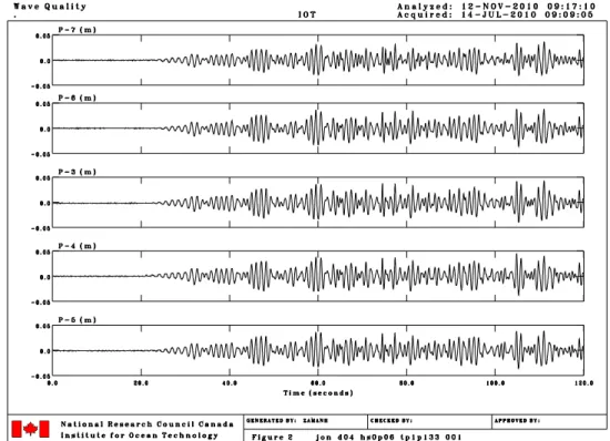
Fig. 6c Surface elevations of FOG at Probe-3 to Probe-7 (d=0.4m, Tp=1.133s and Hs=0.06m)

Fig. 6d Surface elevations of FOG at Probe-1 to Probe-3 and Probe-8 to Probe-9 (d=0.4m, Tp=1.133s and Hs=0.06m)

(26)

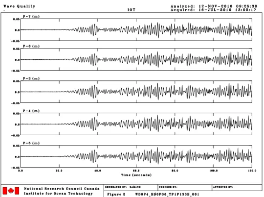
Fig. 6e Surface elevations of SOG at Probe-3 to Probe-7 (d=0.4m, Tp=1.133s and Hs=0.06m)

Fig. 6f Surface elevations of SOG at Probe-1 to Probe-3 and Probe-8 to Probe-9 (d=0.4m, Tp=1.133s and Hs=0.06m)

(27)

(28)

(29)

(30)

(31)

(32)

(33)

(34)

(35)

Fig. 9a Comparisons between primary and low frequency wave components of FOG and SOG spectrum at Probe-14, Probe-1, Probe-2, Probe-3, Probe-8 and Probe-9

(36)

Fig. 9b Comparisons between high frequency wave components of FOG and SOG spectrum at Probe-14, Probe-1, Probe-2, Probe-3, Probe-8 and Probe-9

(37)

(38)

(39)

(40)

(41)

(42)

(43)

(44)

(45)

(46)

(47)

(48)

(49)

(50)

(51)

(52)

(53)

(54)

(55)

(56)

(57)

(58)

(59)

APPENDIX – II

Isolated wave components obtained from both first- and second-order measured wave profiles using Lwave computer codes.

(60)

(61)

Fig. 15a: Isolated wave components for FOG technique at Probe-14 ( d=0.4m, Tp=1.133s, and Hs=0.06m ) Primary Wave Bounded Wave Free wave-1 Free wave-2 Sum waves

(62)

Fig. 15b: Isolated wave components for SOG technique at Probe-14 ( d=0.4m, Tp=1.133s, and Hs=0.06m ) Primary Wave Bounded Wave Free wave-1 Free wave-2 Sum waves

(63)

(64)

(65)

(66)

(67)

(68)

(69)

(70)

(71)

(72)

(73)

(74)

(75)

(76)

(77)

(78)

(79)

(80)

(81)

(82)

(83)

(84)

(85)

(86)

(87)

(88)

(89)

(90)

(91)

(92)

(93)

(94)

(95)

Fig. 32a: Isolated wave components for FOG technique at Probe-9 ( d=0.4m, Tp=2.145s, and Hs=0.06m ) Primary Wave Bounded Wave Free wave-1 Free wave-2 Sum waves

(96)

(97)

(98)

Fig. 33b: Isolated wave components for SOG technique at Probe-14 ( d=0.5m, Tp=1.133s, and Hs=0.06m ) Primary Wave Bounded Wave Free wave-1 Free wave-2 Sum waves

(99)

(100)

(101)

(102)

Fig. 35b: Isolated wave components for SOG technique at Probe-2 ( d=0.5, Tp=1.133s, and Hs=0.06m ) Primary Wave Bounded Wave Free wave-1 Free wave-2 Sum waves

(103)

(104)

(105)

(106)

(107)

(108)

(109)

(110)

(111)

(112)

(113)

(114)

(115)

(116)

(117)

(118)

(119)

(120)

(121)

(122)

(123)

(124)

(125)

(126)

(127)

(128)

(129)

(130)

(131)

(132)

(133)

(134)

(135)

(136)

(137)

(138)

Fig. 53b: Isolated wave components for SOG technique at Probe-2 ( d=0.6, Tp=1.133s, and Hs=0.06m ) Primary Wave Bounded Wave Free wave-1 Free wave-2 Sum waves

(139)

(140)

(141)

(142)

(143)

(144)

(145)

(146)

(147)

(148)

(149)