A Dynamic Key Frames Approach to Object
Tracking
by
Christopher A. Wilkens
Submitted to the Department of Electrical Engineering and Computer
Science
in partial fulfillment of the requirements for the degree of
Master of Engineering in Computer Science and Engineering
at the
MASSACHUSETTS INSTITUTE OF TECHNOLOGY
May 2008
c
Massachusetts Institute of Technology 2008. All rights reserved.
Author . . . .
Department of Electrical Engineering and Computer Science
May 9, 2008
Certified by . . . .
David Demirdjian
Research Affiliate
Thesis Supervisor
Accepted by . . . .
Arthur C. Smith
Chairman, Department Committee on Graduate Students
A Dynamic Key Frames Approach to Object Tracking
by
Christopher A. Wilkens
Submitted to the Department of Electrical Engineering and Computer Science on May 9, 2008, in partial fulfillment of the
requirements for the degree of
Master of Engineering in Computer Science and Engineering
Abstract
In this thesis, I present a dynamic key frames algorithm for state estimation from observations. The algorithm uses KL-divergence as a metric to identify the frames that contribute the most information to estimation of the system’s current state. The algorithm is first presented in a numerical optimization framework and then developed as an extension to the Condensation algorithm. Finally, I present results from a Matlab simulation of the algorithm.
Thesis Supervisor: David Demirdjian Title: Research Affiliate
Acknowledgments
Special thanks go to Dr. David Demirdjian who was my research advisor over the past year and to Professor Trevor Darrell who supported me and funded much of my research.
Contents
1 Introduction 13
1.1 Challenges . . . 14
1.2 Existing Work . . . 15
2 The DKF Algorithm 19 2.1 Multiple Target Tracking . . . 22
2.2 Condensation-DKF . . . 23
3 Implementation and Results 27 3.1 Data Sets . . . 28 3.2 Benchmarks . . . 29 3.2.1 Kalman Filter . . . 29 3.2.2 Condensation . . . 31 3.3 Numerical Optimization . . . 32 3.4 Condensation DKF . . . 34 3.5 Results . . . 36
4 Conclusion and Further Work 39 A Matlab Code 41 A.1 Generating Data . . . 41
A.2 Testing Framework . . . 50
A.3 Posterior Probabilities . . . 56
A.5 Condensation and Condensation DKF . . . 74 A.6 Kalman Filter . . . 86 A.7 Utility Functions . . . 90
List of Figures
2-1 At each step, the algorithm keeps the frames most influential to the distribution of Zt. . . 20
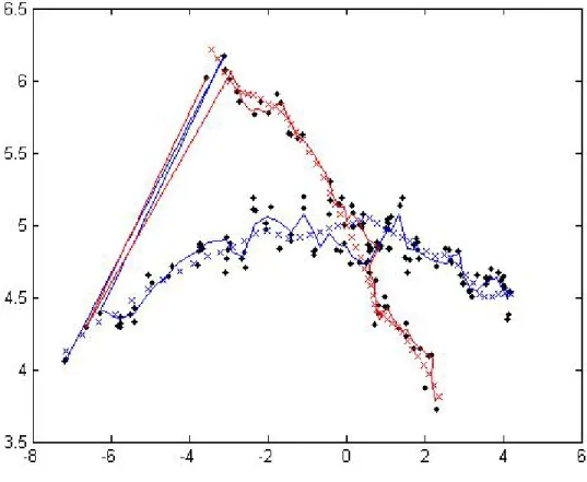
3-1 In this run, two objects move from left to right through an image. The ground truth positions are denoted with an ’x’ while the observations are denoted with a ’.’. The red object is occluded for a long period of time and reappears just on the other side of the blue object, making successful tracking difficult. . . 28 3-2 Tracking with a Kalman filter. The solid red and blue lines represent
the estimated trajectories computed by the Kalman filter as the objects move down and to the right. The data association used for the Kalman filter forced it to recover the red trajectory; however, it switched the two objects. . . 30 3-3 Tracking with Condensation. The two solid lines represent a failed run
of the condensation filter. The occlusion is too long and the red trajec-tory cannot recover, while the blue hypothesis goes halfway between the red and blue objects. . . 31 3-4 DKF keeping all frames. The solid red and blue lines represent the
trajectories estimated by the algorithm and the rainbow colored lines represent the optimal partial trajectories found at each timestep. The temporary crossover at the beginning occurs in step 2 because estimat-ing two trajectories from four points is ambiguous. . . 33
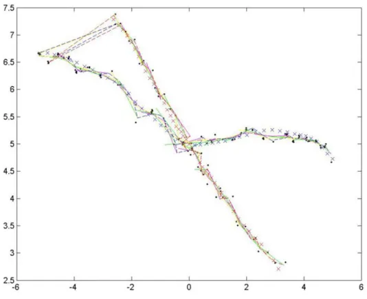
3-5 DKF keeping the last four frames. The dashed red and blue lines repre-sent the trajectories estimated by the algorithm. The rainbow colored lines represent the optimal partial trajectories found at each timestep. When we keep the last four frames, we are optimizing our trajectory estimate over only those frames, causing the scarcity of partial trajec-tories through the occlusion. . . 35 3-6 DKF using four frames and the Euclidean distance metric. The dashed
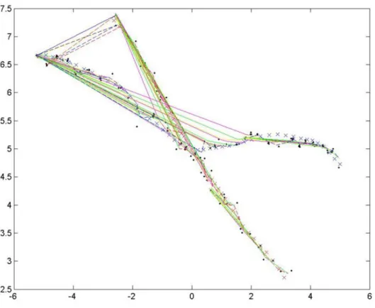
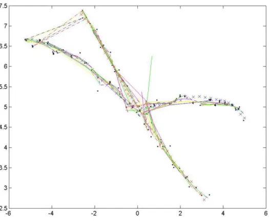
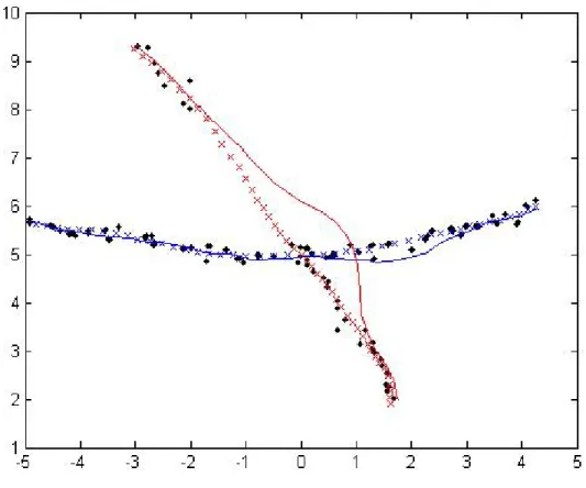
red and blue lines represent the trajectories estimated by the algorithm and the rainbow colored lines represent the optimal partial trajectories at each timestep. With this metric, the algorithm may elect to keep older observations, giving rise to longer partial trajectories than when only the last four frames were kept (see figure 3-5.) The Euclidean distance metric likes to keep the first observation around for a long time, which generates the long rays seen around the intersection. . . . 36 3-7 DKF using four frames and the KL-divergence metric. The solid red
and blue lines represent the trajectories estimated by the algorithm and the rainbow colored lines represent the optimal partial trajecto-ries found at each timestep. Like the Euclidean distance metric, the KL-divergence metric elects to keep observations before the occlusion; however, it is more intelligent and does not simply keep the first ob-servation. . . 37 3-8 Condensation DKF using four frames and the KL divergence metric.
The solid red and blue lines represent the trajectories estimated by the algorithm. Compared to the standard Condensation filter on the same data in figure 3-3, the DKF implementation has less of a tendency to get confused as it approaches the blue trajectory and is able to pick up the red object when it reappears. . . 38
List of Tables
3.1 The DKF approaches performed well, with performance among the DKF variants commensurate with expectations. . . 38
Chapter 1
Introduction
Many problems in signal processing and artificial intelligence may be framed as state estimation from past observations. One such task is object tracking. In object track-ing, the path of an object is estimated as the object moves through a series of camera frames.
Object tracking is an important task in machine vision. It is useful for a wide variety of tasks from 3D from-motion to video surveillance. In 3D structure-from-motion, we track known points on a 3D object. Then, the 3D structure of those points is inferred from their trajectories. In video surveillance, one could track people of interest and look for suspicious behavior. Similarly, one could track the players in a sporting event. Finally, at a more basic level, object tracking may be used as a means of locating an object in an image during a time when it is occluded, increasing machine intelligence by allowing a computer to understand that an object has not entirely disappeared just because it is not visible.
In this thesis, we will develop a new algorithm for state estimation that provides an efficient way to identify and save relevant historical observations in order to improve tracking robustness. Then we will test our algorithm in simulation.
1.1
Challenges
Many algorithms perform quite well when tracking particular objects under controlled conditions. Unfortunately, object tracking in the general case remains an open prob-lem. Background clutter, partial occlusions, unusual perspectives, lighting, and many other factors make reliable image understanding and tracking extremely difficult.
Some properties that commonly confound state estimation are nonlinear dynam-ics and complex probability distributions. Unfortunately, both are present in object tracking. A moving object, such as a person, may follow a highly nonlinear dy-namic model. Nonlinear dydy-namics, while not necessarily intractable, make efficient algorithms for state estimation scarce.
The probability distributions present in object tracking are also very complex. For example, in the presence of image clutter, a tracking algorithm may see a plu-rality of objects that look like the one it was tracking, generating highly multimodal distributions. The problem is magnified when tracking multiple targets, as the image always has a plurality of similar objects.
Occlusions, or frames where the object of interest is hidden behind another object, present another difficult problem. While the temporary loss of data would reflect a failure in many systems, it is a natural occurrence when multiple objects interact in a scene. A successful tracking algorithm must be able to understand the object’s dynamics and predict the location of the object even when it is completely hidden or only partially visible so that it can recover tracking when the object reappears.
Some other difficulties of object tracking are inherent to object detection and image understanding. Varying image conditions may make accurate detection and localization quite difficult and generate a significant amount of noise. The exact location of an object may vary from frame to frame based on subtle changes in its identifying features and even the discretization implicit in the digital image. For example, lighting fluctuations on a shadowed edge of an object may significantly affect the perceived boundary, generating substantial noise in the observed center of the object.
We will demonstrate a general framework that is able to handle these difficulties more effectively than existing algorithms.
1.2
Existing Work
Many solutions to the object tracking problem have been attempted with varying success. In theory, the best approach would use all historical observations in a batch optimization to estimate the object’s current location. Unfortunately, this quickly becomes intractable because the data set grows linearly with time.
To efficiently track objects, many people have developed recursive Bayesian algo-rithms [10][8][17][6]. These algoalgo-rithms assume Markovianity of the object’s position process and compute the posterior probability distribution, i.e. the probability dis-tribution over the current location of the object, from the disdis-tribution at the last frame and the current image. This gives a recursive form to the solution, rendering the resulting problem tractable.
One of the earliest such algorithms used for object tracking is the Kalman fil-ter [10]. The Kalman filfil-ter is an optimal, recursive estimator for linear Gaussian systems. Consequently, if the input observations are best modeled by a linear Gaus-sian system, this will work very well. Unfortunately, as we have already discussed, dynamics are frequently nonlinear and distributions are often multimodal. The details of the Kalman filter are discussed in section 3.2.1.
The Kalman filter has been extended to handle nonlinear dynamics and subse-quently applied to object tracking in more complex situations [9]. The extended Kalman filter (EKF) extends this idea to include nonlinear dynamics by using linear approximations when propagating the covariance. Unfortunately, it is neither an opti-mal estimator nor proven to converge, so it may be useless in other applications. The Unscented Kalman Filter (UKF) of Julier et al. [9] builds on the EKF by elegantly propagating both the mean and the covariance through the nonlinear system. This addresses some nonlinear dynamics issues, but it still requires Gaussian distributions. In order to handle image clutter, Shalom et al. developed the probabilistic data
association filter (PDAF) [17][6]. The PDAF is a Bayesian algorithm that can prob-abilistically handle multiple observations in the vicinity of the object being tracked. The PDAF incorporates the probability that a particular observation was generated by the desired object, giving it more flexibility than all-or-nothing approaches.
A more recent development in recursive Bayesian algorithms adopts the idea of a particle filter [8][15]. Issard and Blake’s Condensation algorithm permits arbitrarily complex posterior distributions and dynamic models at a reasonable cost in accuracy and efficiency [8]. In practice, the Condensation algorithm performs fairly well in many contexts. Its ability to maintain arbitrarily complex distributions allows it to handle the complex posteriors that frequently occur in noisy and occluded object tracking settings. We will extend this algorithm in section 2.2.
However, the Markovian assumption is frequently wrong. To handle these cases, some have attempted to apply semi-Markovian models to other tracking environ-ments [12]. A semi-Markov process is similar to a Markov one, except that the time between state transitions may be distributed according to a more general probabilis-tic distribution (as opposed to the geometric form inherent in a standard Markov process.) Such models offer significant power but require model-specific recursive algorithms. In contrast, our approach only assumes smoothness.
Some tracking algorithms take a different approach and focus on developing ac-curate models of the item being tracked [11][1][18]. For example, human motion tracking algorithms will frequently use a model of the human body to improve per-formance. An extreme example is the SCAPE model which uses a detailed 3D surface model to estimate human pose and track motion accurately [1]. Similarly, the feature-based algorithm of Shi and Tomasi tracks objects by analyzing the motion of model features from frame to frame [18]. These approaches may work well, but like the semi-Markovian models, they are very task- and situation-specific. In particular, they require a good model a priori, and, in many cases, it is difficult or impossible to construct such a model.
Another body of research has tackled the problem of simultaneously tracking multiple targets. One of the biggest challenges with multiple target tracking is the
data association problem: determining the correspondence between observations and targets.
In many ways, the problem is similar to that of tracking objects in clutter. An algorithm must decide whether or not a particular observation corresponds to the current trajectory, with the new constraints that an object may belong to one of many trajectories. Given this similarity, a natural approach to multiple target track-ing was to extend the PDAF to handle multiple targets [7]. The resulting joint probabilistic data association filter (JPDAF) has been used and extended in many multi-target tracking applications, including tracking contours with HMMs [3] and mobile robotics [5].
One fundamental approach is multiple hypothesis tracking (MHT) pioneered by Reid [16]. MHT maintains a set of trajectories based on particular observation-target associations. Unfortunately, the number of possible assignment sets grows exponentially with time. Consequently, much of the ongoing work in MHT revolves around efficient approximations and heuristics. For example, Cox and Hingorani keep only the k best trajectories [4], and Vasquez and Williams exploit correlation effects [20].
A more recent idea applies Markov chain Monte Carlo simulation to the tracking problem [14]. These methods have become possible with the increased power of modern computers and have produced strong results.
While most approaches to multiple target tracking involve data association, the task may be circumvented through alternative statistical techniques. For example, network tomography infers global trajectories from local movements without explicitly identifying objects. Boyd and Meloche use this approach to track pedestrians at a crowded intersection [2].
Finally, another set of tracking algorithms use a key frames approach. A small subset of observations is kept and used to track in a manner similar to batch process-ing. Vacchetti et al. [19] and Morency et al. [13] use heuristics or hand labeling to identify representative views of an object as their key frames. At any given step, these views are used to estimate the location and perspective of the object being tracked.
When necessary, the key frame set is updated using heuristics.
In contrast, our dynamic key frames algorithm (DKF) keeps the locally optimal frames for estimating both the current location and dynamics of the object. At each step, the algorithm computes and saves the set of key frames most relevant to its understanding of the system’s state. This gives more robustness than either the Bayesian recursive algorithms or the existing heuristic-based key frames approaches. In the following chapters, we will describe the design and implementation of DKF. Chapter 2 discuss the theory behind the algorithm and formulates it in the particle filter framework of Condensation. Chapter 3 discusses our implementation of both a batch DKF version and the Condensation DKF algorithm. Finally, in chapter 4 we conclude and recommend future work.
Chapter 2
The DKF Algorithm
We propose a general application of the key frames paradigm to estimate state from observations. It will maintain a dynamic active set of key frames chosen to maximize the amount of information known about the current state of the system. At each step, the algorithm will estimate the system’s current state and use Kullbak-Leiber divergence (KL-divergence) computations to determine which frames in the active set are most relevant.
Formally, we wish to estimate the trajectory Xt = {x0, . . . xt} from image
obser-vations I0, . . . It. A global optimization routine seeks to optimize the full posterior.
Namely, it seeks to find the optimal estimate ˆxt of the current state xt given all
previous frame data:
ˆ
x0. . . ˆxt= argmax x0,...xt
P (x0. . . xt|I0, . . . It).
In contrast, a recursive Bayesian optimization solution assumes Markovianity, giving the following factorization of the joint posterior:
P (x0, . . . , xt|I1, . . . , It) = P (x0) k
Y
i=1
P (Ii|xi) · P (xi|xi−1).
filter:
P (xt|It−1) =
Z
P (xt|xt−1)P (xt−1|It−1) dxt−1
P (xt|It) = α P (It|xt)P (xt|It−1)
Our approach will take a middle ground, optimizing over a small active set AS = {I1, I2, . . . Ik} of frames, i.e.
ˆ
xt1, . . . ˆxtkxˆt= argmax
xt1,...xtk,xt
P (xt|AS).
Finally, we take the estimate of the current state to be ˆx as computed above. For notational purposes, let Zt be the posterior distribution over possible positions xt of
an object in an image at time t and ˆx(Zt) be the best estimate of xt from Zt. Also,
Zt(S) be the distribution over possible positions xtbased on dynamic constraints and
a set of frames S, and ˆx(S) = ˆx(Zt(S)) as shorthand. In essence,
Zt(AS) ∼ P (xt|AS).
Figure 2-1: At each step, the algorithm keeps the frames most influential to the distribution of Zt.
frames most relevant to our knowledge object’s current position. At a high level, the algorithm may be summarized as follows:
1. Incorporate the current frame, ft, by adding it to the active set, ASt= ASt−10 ∪
{ft}.
2. Estimate xt from the frames in the active set as ˆx(ASt).
3. Discard frames to keep the active set small, i.e. ASt0 = SELECT (ASt).
The key to making the algorithm work well is to design SELECT (ASt) to keep the
most useful frames from ASt. Our goal is to demonstrate the superiority of a
KL-divergence based SELECT . In this thesis, we elect to keep exactly k frames from step to step and compare a few different approaches:
1. Keep the last k frames. This gives
SELECT (ASt = {It1, . . . , Itk, It}) = {It2, . . . , Itk, It}
2. Keep the k frames that minimize the Euclidean distance between ˆx(ASt) and
ˆ
x(ASt0), i.e.
SELECT (ASt= {It1, . . . , Itk, It}) = ASt− argmin
Ij∈ASt
|ˆxt(ASt) − ˆxt(ASt− Ij)| .
3. Keep the k frames that minimize the KL-divergence between Zt(ASt) and
Zt(ASt0), i.e.
SELECT (ASt= {It1, . . . , Itk, It}) = ASt−argmin
Ij∈ASt
DKL(Zt(ASt−Ij) − Zt(ASt))
where DKL(·) is defined as DKL(Zt( ˜ASt)kZt(ASt)) = Z pZ t( ˜ASt)(x) log pZt( ˜ASt)(x) qZt(ASt)(x) dx
or as DKL(Zt( ˜ASt)kZt(ASt)) = X pZ t( ˜ASt)(x) log pZ t( ˜ASt)(x) qZt(ASt)(x)
for discrete distributions.
4. Keep all the frames.
We expect the KL-divergence to have the best performance of the tractable SELECT implementations. The KL-divergence measures the distance between the Zt distributions, thereby approximating the information from all the frames in ASt
as well as possible.
In contrast, keeping the last k frames fails to consider the relevance of the obser-vations. For example, occlusions frequently happen for significant, contiguous blocks of time. If an object is occluded for more than k frames, keeping the last k frames is of little added benefit. One might employ a heuristic to determine that the current frames were empty, but the other approaches solve the problem more generally.
Minimizing the Euclidean distance provides some measure of relevance when se-lecting the active set. Its weakness is that it only propagates the mode of Zt. At
each step, the algorithm is forced to commit to a particular trajectory assignment and picks frames that will, in the future, bias it toward that choice. Thus, while it may handle occlusions well, it will likely fail when it is important to maintain the multimodality of Zt.
Finally, as previously noted, keeping the entire frame history in the active set is computationally intractable. However, it is a useful performance benchmark that we will use later.
2.1
Multiple Target Tracking
One of our goals in this work is to demonstrate the performance of DKF when simul-taneously tracking multiple targets. To simulsimul-taneously track, we augment Xt (and
therefore xt) to include the position of all objects being tracked, e.g. xt= x1 t x2t .. .
where xjt is the location of object j at time t. This sacrifices efficiency for accuracy, as it significantly increases the dimensionality of the tracking space. In the future, when we refer to X, xt, and ˆx, we are referring to the concatenation of of the locations and
estimates for all objects being tracked.
This complicates our computation of ˆxt. In general, using the instantaneous mode
of a multimodal distribution is potentially unstable because the estimate may jump between modes. In the case of multiple targets, this manifests itself as ˆxt jumping
between trajectories.
2.2
Condensation-DKF
In order to practically implement dynamic key frames, we need to give efficient ways to compute ˆx and SELECT (ASt). Instead of seeking an analytic solution, we will
seek a numerical approximation using a particle filter. Specifically, we will extend the Condensation algorithm. This will give us arbitrary (theoretical) precision in a simple implementation.
Issard and Blake’s Condensation algorithm [8] is a standard, weighted particle filter resampled at each timestep. At time t, we start with the weighted samples from the previous step, {s(n)t−1, πt−1(n)} where s(n)t−1 corresponds to sample n and πt−1(n) is the weight for sample n. We sample from this distribution and do a randomized prediction to get the next set of samples, {s(n)t }. Finally, we compute new weights based on the current image.
The algorithm can be summarized as follows:
get a set of particles {s0(n)t−1}.
2. Drift and diffuse. Deterministically predict the next location for each particle and add noise to each sample according to the dynamic model. This gives {s(n)t }.
3. Weight. Compute new weights {π(n)t−1} = {P r(s(n)t |It)}, i.e. the conditional
probability of the sample given the current frame.
At the sampling stage, the particles will be distributed according to P r(s(n)t−1|Zt−1).
In the drift and diffusion stage, the probability of getting a particular sample s(n)t can be written as P r(s(n)t |s(n)t−1). The algorithm is implemented such that this conditional probability matches the system dynamics. This gives samples {s(n)t } distributed ac-cording to
P r(s(n)t |s(n)t−1) · P r(st−1(n)|Zt−1) = P r(s(n)t |Zt−1).
Finally, the weights are then chosen to be {πt−1(n)} = {P r(s(n)t |ft)}. This implies
that the final weighted particle distribution is a representation of
P r(s(n)t |Zt−1∩ ft).
In the limit as the number of particles grows, the collection will approach the true distribution, thus making the Condensation algorithm a correct recursive estimator.
The only remaining task is to estimate ˆxtfrom Zt. For this thesis, we compute ˆxt
as the mode of Zt. As noted earlier, this is slightly problematic.
Now, we are ready to define Condensation-DKF. We extend our samples to include a trajectory over the frames in the active set. Previously, condensation samples contained only position and velocity information for the object at time t. Now, samples will also include position information for each of the frames contained in the active set.
Conveniently, the computation of ˆx does not change from a traditional condensa-tion implementacondensa-tion. It is computed as the instantaneous mode of Ztby ignoring the
Now, we need to show how to implement DKF. First, in order to compare two potential active sets, we need a way to represent Zt( ˜ASt) where ˜ASt⊂ ASt. For this,
we keep the same particles, discard information for frames not in ˜ASt, and compute
new weights πn ˜
AS. This gives us an approximation of Zt( ˜ASt).
When using the Euclidean distance metric, we can compute ˆx( ˜ASt) and pick the
best subset ˜ASt.
Computing the KL-divergence is slightly more difficult. The distribution Zt is
ideally continuous. This gives us the following form for the KL-divergence:
DKL(Zt( ˜ASt)kZt(ASt)) = Z pZ t( ˜ASt)(x) log pZ t( ˜ASt)(x) qZt(ASt)(x) dx.
However, we cannot easily compute this function in continuous space, so we would like to use the discrete version as an approximation. The easy approach is to perform the sum such that each sample trajectory sn
t corresponds to a point in the sum, i.e.
DKL(Zt( ˜ASt)kZt(ASt)) = X n αnAS˜ log βn ˜ AS γn AS
for some appropriate α, β, and γ. We observe that the total probability of a trajectory selected this way is δn·πn
S, where S is the active set being used and δ is the probability
implicitly encoded in the particle distribution. This suggests that we take
α = β = δn· πn ˜ ASt.
However, if we add over all samples, a multiplicative factor of δnis implicitly present.
Thus, we actually want
α = πASn˜ t, β = δnt−1· πn ˜ ASt, and γ = δnt−1· πASn t.
This gives the final form DKL(Zt( ˜ASt)kZt(ASt)) = X n πASn˜ tlog δn t−1· πnAS˜ t δn t−1· πASn t .
which conveniently simplifies to
DKL(Zt( ˜ASt)kZt(ASt)) = X n πASn˜tlog πASn˜ t πn AS
Chapter 3
Implementation and Results
To test the DKF approach, we implemented it in Matlab and tested it against sim-ulated data sets. The simulation trajectories were designed to have the following difficult properties related to object tracking:
1. Occlusion. In each trial, one trajectory has a significant (≈ 10 frame) occluded region.
2. Clutter. In cluttered environments, there may be many candidate observations near a given trajectory. In our tests, one trajectory is cluttered, containing multiple observations near the object.
3. Multiple targets. Each trial contains two separate intersecting trajectories. The trajectories are intended to represent similar objects, so the recognition stage cannot differentiate between them.
4. Noise. We add Gaussian noise to simulate standard measurement noise.
For the test trajectories, an “image” is simply a collection of locations (xi, yi)
corresponding the locations of an object. Such data could presumably be obtained by running an object detection scheme first.
3.1
Data Sets
Tests were primarily conducted on an occluded intersection data set of 100 trials. In this data set, the first trajectory is occluded as it passes by the second trajectory (see figure 3-1.) The second trajectory is “cluttered” at each timestep with an average of one extra observation near the trajectory. Finally, Gaussian noise is added to each trajectory.
Figure 3-1: In this run, two objects move from left to right through an image. The ground truth positions are denoted with an ’x’ while the observations are denoted with a ’.’. The red object is occluded for a long period of time and reappears just on the other side of the blue object, making successful tracking difficult.
3.2
Benchmarks
As a benchmark, we implemented the standard Kalman filter and the Condensation algorithm.
3.2.1
Kalman Filter
As mentioned earlier, the Kalman filter is an optimal recursive estimator for linear Gaussian systems. It may be derived fairly easily, but we will just summarize the results. First, one must model their system using linear state update equations as
xt= A · xt−1+ wk−1
yt= C · xt+ vt
where xt is the internal state at time t, yt is observed, and wt ∼ N (0, Q) and
vt ∼ N (0, R) are Gaussian noise variables. The resulting Kalman filter consists
of prediction and update equations for both the mean, ˆx, and the covariance, P . Prediction: ˆ xt|t−1 = Akxˆt−1|t−1 Pt|t−1 = APt−1|t−1AT + Q. Update: Kt = Pt|t−1CT(CPt|t−1CT + R)−1 ˆ xt|t−1+ Kt(yt− C ˆxt|t−1) Pt|t = (I − KtC)Pt|t−1
The prediction equations predict the mean ˆxt|t−1 and covariance Pt|t−1 of the
distribution of xt given the distribution at time t − 1. Then, the update equations
adjust this prediction based on the actual observations at time t.
the state space to include the locations of two objects and to identify observations with a particular trajectory. To enable multiple target tracking, observations were assigned to trajectories before updating ˆx based on the current frame. To do this, we used a nearest-neighbors approach and assigned observations to the closest trajectory. A sample trial using the Kalman filter is in figure 3-2.
Figure 3-2: Tracking with a Kalman filter. The solid red and blue lines represent the estimated trajectories computed by the Kalman filter as the objects move down and to the right. The data association used for the Kalman filter forced it to recover the red trajectory; however, it switched the two objects.
A key weakness of the Kalman filter in these tests was its inability to represent multimodal distributions. At the intersection, the Kalman filter could not represent the multimodality that appears in Zt. (I.e. did the paths cross or did the objects turn
away from each other at the last minute?) In combination with the early assignment of observations, this causes the Kalman filter to follow the cluttered trajectory instead of waiting for the other trajectory to stop being occluded. The success rate for the
Kalman filter was a mere 24% (see table 3.1.)
3.2.2
Condensation
Similar to the Kalman filter, Condensation was implemented using an extended state space to store the position of both objects. In our implementation, each sample also stored the velocity of the object for prediction purposes. To compute ˆx from the samples, we used an implementation of the mean-shift algorithm to find the mode of Zt.
As noted earlier, the mode of Zt is not necessarily stable in a particle filter. This
can be clearly seen in the results as the hypothesis hops between trajectories.
Figure 3-3: Tracking with Condensation. The two solid lines represent a failed run of the condensation filter. The occlusion is too long and the red trajectory cannot recover, while the blue hypothesis goes halfway between the red and blue objects.
3.3
Numerical Optimization
Our first implementation of DKF used Matlab’s numerical optimization methods. Specifically, we wrote a function
α (xt1, . . . , xtk, xt) = P r (xt1, . . . , xtk, xt|ASt)
where
ASt = {It1, . . . , Itk, It}.
We use Matlab’s built-in Levenberg-Marquardt optimizer to find
˜
Xt = argmax xt1,...,xtk,xt
α(xt1, . . . , xtk, xt).
Unfortunately, α is symmetric: as defined, trajectories may be arbitrarily inter-changed while maintaining the same α value. Consequently, after finding ˜Xt, we
must match the trajectories. For this, we take the Euclidean distance between the overlapping points in Xt−1 and ˜Xt and compute the minimal matching. Finally, we
append the final value of ˜Xt to Xt−1 to get Xt.
In this case, computing the posterior probability of a path includes associating observations with trajectories. This gives it a significant advantage, allowing it do isolate the two trajectories with near perfection when they were both visible.
Unfortunately, the myriad local minima of the optimization space made this ap-proach somewhat difficult. Matlab was highly effective at optimizing paths once the observations were associated with the correct trajectory; however, all of Matlab’s built-in optimization algorithms rarely changed more than a couple observation as-sociations from their values in the initialization vector. As a result, we needed to carefully select the initialization vector.
We finally used dynamic programming to construct the initialization trajectories. We used a modified construction of the Viterbi algorithm that evaluated the total posterior (instead of multiplying the conditional by the previous probability) to
con-struct two trajectories entirely from observation points and interpolated occlusions. (Note that these trajectories are not optimal in any overall sense - they are merely a good starting point.)
Fortunately, due to the method by which trajectories were matched to the past, this implementation did not suffer from the instability seen in the Condensation algorithm. The only exception is the second frame, where the optimizer almost always switched the two trajectories briefly.
Ultimately, when the optimization trackers erred, they swapped trajectories at the intersection. For this problem, the optimizer was largely at the mercy of the initialization vector.
Figure 3-4: DKF keeping all frames. The solid red and blue lines represent the trajectories estimated by the algorithm and the rainbow colored lines represent the optimal partial trajectories found at each timestep. The temporary crossover at the beginning occurs in step 2 because estimating two trajectories from four points is ambiguous.
As one would expect, the approach that kept the entire history in the active set performed the best, successfully tracking both objects 68% of the time (see figure 3-4 and table 3.1.) On the other hand, the routine that kept only the last four frames (see figure 3-5) performed significantly worse, successfully tracking only 55% of the frames. It is worth noting that the implementation of the batch processor was extremely robust to the replicated trajectory. It was rarely fooled more than temporarily by the replicated trajectory in the same way as the Kalman filter. Consequently, the difference in the DKF implementations lies in their ability to track objects through the occluded intersection and recover the correct path in the end. Thus, the basline for an algorithm that randomly guessed is 50% and, therefore, the difference between 55% and 68% is much larger than it might seem at first glance.
The two intelligent DKF schemes demonstrated a significant improvement. Se-lecting frames based on the Euclidean distance metric kept frames that gave more information about the occluded intersection point (see figure 3-6.) On the other hand, it did not always keep the most logical frames. For example, in the blue example tra-jectory, the first frame is kept for a long time. (This is evidenced by the rainbow colored partial paths that can be seen reaching from the first observation past the intersection point.) The KL-divergence metric made more reasonable decisions - the partial paths show that it generally kept more recent observations, as one would ex-pect. The success rates corroborate the intuitive notions, with a 60% success rate for the Euclidean metric and a 64% success rate for the KL-divergence metric.
Overall, the results from numerical optimization were quite promising. On this type of data set, at least, DKF with the KL-divergence metric stands to provide a significant enhancement over existing algorithms.
3.4
Condensation DKF
For our final tests, we implemented the Condensation variant of DKF as described in chapter 2. In the Condensation filter, the performance difference was less obvi-ous. The raw success rate was about the same, though the DKF variant generally
Figure 3-5: DKF keeping the last four frames. The dashed red and blue lines represent the trajectories estimated by the algorithm. The rainbow colored lines represent the optimal partial trajectories found at each timestep. When we keep the last four frames, we are optimizing our trajectory estimate over only those frames, causing the scarcity of partial trajectories through the occlusion.
produced smoother, more accurate trajectories (the results in table 3.1 do not reflect this because they use a boolean quantity for success.)
The discrepancy is likely due to the incomparability of particle counts and the method of measuring success. The added dimensionality in the DKF variant requires more particles to accurately handle the distribution; however, it is not clear that this makes a fair comparison. For the purposes of this thesis, we used the same number of particles (5000) for both the standard and DKF versions of Condensation.
Figure 3-6: DKF using four frames and the Euclidean distance metric. The dashed red and blue lines represent the trajectories estimated by the algorithm and the rainbow colored lines represent the optimal partial trajectories at each timestep. With this metric, the algorithm may elect to keep older observations, giving rise to longer partial trajectories than when only the last four frames were kept (see figure 3-5.) The Euclidean distance metric likes to keep the first observation around for a long time, which generates the long rays seen around the intersection.
3.5
Results
The results (see table 3.1) were generally as anticipated. The simple benchmark approaches could not reliably handle the occlusions and replications. These were handled much more effectively by batch DKF implementations. Success across the different DKF implementations varied as expected, and the KL-divergence metric yielded performance amazingly close to the version that kept the entire history.
Unfortunately, the Condensation DKF version did not perform as well as expected, likely because of incomparable particle counts. In general, the DKF version produced
Figure 3-7: DKF using four frames and the KL-divergence metric. The solid red and blue lines represent the trajectories estimated by the algorithm and the rainbow colored lines represent the optimal partial trajectories found at each timestep. Like the Euclidean distance metric, the KL-divergence metric elects to keep observations before the occlusion; however, it is more intelligent and does not simply keep the first observation.
smoother, more accurate trajectories but was still susceptible to getting lost when run with comparatively low particle counts.
We defined a successful run as one in which the data association was correct for 80% of the run. When the batch methods erred, they handled the occlusion but switched trajectories at the intersection. Consequently, they were well above or below the 80% cutoff.
In contrast, the Kalman filter and condensation algorithms were closer to the cutoff. The trajectories would frequently merge around the occluded intersection and split again a while later.
Figure 3-8: Condensation DKF using four frames and the KL divergence metric. The solid red and blue lines represent the trajectories estimated by the algorithm. Compared to the standard Condensation filter on the same data in figure 3-3, the DKF implementation has less of a tendency to get confused as it approaches the blue trajectory and is able to pick up the red object when it reappears.
Benchmarks Kalman Filter 24%
Condensation 50% DKF (|AS| = 4) All-frames 68% Most recent 55% Euclidean 60% KL-Divergence 64% Condensation-DKF (|AS| = 4) KL-Divergence 49%
Table 3.1: The DKF approaches performed well, with performance among the DKF variants commensurate with expectations.
Chapter 4
Conclusion and Further Work
The simulation results demonstrated that batch DKF using the KL-divergence met-ric in the simulation environment is a good approximation of full batch processing, even with an active set of only four items. It was able to successfully track objects through occlusions, intersections, and duplications that more frequently fooled other algorithms.
The key to the success of DKF is its selection of the most relevant frames. By using the KL-divergence to compare posterior distributions, it saves the locally optimal set of key frames from step to step and uses those frames to find the optimal estimate.
Unfortunately, the Condensation DKF implementation demonstrated weaker re-sults than the batch implementation. It generally produced smoother estimates that were closer to the ground truth than the traditional Condensation algorithm, but it did not demonstrate the extra resilience to occlusions and intersections that the batch version did.
One of the key benefits to our approach is its simple generality. The algorithm requires minimal assumptions about the structure of the input. One need only specify the posterior function α to track in entirely different contexts. In a more general way, this methodology can be easily applied to any problem involving state estimation from observations with minimal effort.
The next stage of this work would be to test DKF in a real system and to try a faster implementation. A good source of test data would be a soccer match or traffic
scene, where many identical targets move around the field with fairly complicated dynamics.
One problem with the current implementation is its speed. The Condensation DKF implementation requires about 20 seconds to process each frame on an Intel 2.6GHz Core2 processor when run with 5000 particles. In large part, this is because it was implemented inefficiently in Matlab. As a result, the runtime is impractical for any real-time application. To legitimately evaluate Condensation-DKF, it should be implemented in a manner that ensures reasonable performance.
Finally, on a theoretical level, it would be interesting to see if any process structure will give a convenient, closed-form solution for optimization of ˆxt and ASt0.
Overall, while our approach has not yet reached practicality, it is a useful frame-work that may be easily and powerfully applied to many different situations to im-prove tracking performance.
Appendix A
Matlab Code
This appendix contains the Matlab code used for the simulation. The code used to generate the datasets follows immediately in section A.1. The code for the testing framework is in section A.2. After that, section A.3 contains code for computing the posterior probabilities from observations. Sections A.4, A.5, and A.6 contain the implementations of the batch, Condensation, and Kalman algorithms respectively, and, finally, section A.7 contains for various utility functions.
A.1
Generating Data
genData 3D.m
% Generates ground truth data with an occluded intersection: % - two, intersecting trajectories
% - one trajectory is occluded around the intersection
% - the other trajectory exhibits multiple data points for a given
% truth point.
%
% gt - the ground truth data
% obs - the "observations" of the ground truth % tstamps - the time stamps for the observations % init0 - the starting locations of the trajectories
function trajectory = genData_3D(L, dyn_mode)
tstamps = generateTimestamps(L);
x10 = [0 5 2]’; % the location of intersection for the two trajectories
param1 = [0.2 0 0]’; % the velocity of the first trajectory at the intersection param2 = [0.1 -0.1 .1]’; % the velocity of the second trajectory at the intersection
gt1 = simulateTrajectory(dyn_mode, L, x10, param1); % ground truth
gt2 = simulateTrajectory(dyn_mode, L, x10, param2); % ground truth
gt = [gt1 gt2];
[dim one] = size(x10); num_targ = 2;
obs1 = addNoise(gt1, 0.1); % observations
obs2 = addNoise(gt2, 0.1); % observations
init0 = [obs1{1};obs2{1}];
o1split = 4;%ceil(3*rand()); o1splitlvl = .15*rand();
o2occs = ceil(L/5)+ceil(L/3*rand()); o2occf = ceil(L/3*rand())+o2occs;
data_stat = [o1split o1splitlvl o2occs o2occf];
obs1f = split(obs1,L,o1splitlvl,o1split);%occlude(obs1, L, 10, 15); obs2f = occlude(obs2, L, o2occs, o2occf);%obs2;
obs = mergeObservations(obs1f,obs2f);
% obs = addBackgroundNoise(obs,.25,-5,5, 0, 10);
trajectory = struct(’L’, L, ’dim’, dim, ’num_targ’, num_targ,...
’dyn_mode’, dyn_mode, ’gt’, {gt}, ’obs’, {obs}, ’tstamps’, {tstamps},... ’init0’, {init0}, ’data_stat’, {data_stat});
end
genData NM.m
function trajectory = genData_NM(L, dyn_mode)
tstamps = generateTimestamps(L);
x10 = [0 5]’; % the location of the midpoint of the first trajectory x20 = [0 6.25]’; % the location of the midpoint of the second trajectory param1 = [0.2 0]’; % the velocity of the first trajectory at the intersection
[dim one] = size(x10); num_targ = 2;
gt1 = simulateTrajectory(dyn_mode, L, x10, param1); % ground truth
gt2 = simulateTrajectory(dyn_mode, L, x20, param1); % ground truth
gt = [gt1 gt2];
obs1 = addNoise(gt1, 0.1); % observations
obs2 = addNoise(gt2, 0.1); % observations
% o1split = 4;%ceil(3*rand()); % o1splitlvl = .15*rand();
o2occs = ceil(L/5)+ceil(L/3*rand()); o2occf = ceil(L/3*rand())+o2occs; %
% data_stat = [o1split o1splitlvl o2occs o2occf];
obs1f = obs1;%split(obs1,L,o1splitlvl,o1split);%occlude(obs1, L, 10, 15); obs2f = occlude(obs2, L, o2occs, o2occf);%obs2;
obs = mergeObservations(obs1f,obs2f);
%obs = addBackgroundNoise(obs,.25,-5,5, 0, 10);
data_stat = [];
trajectory = struct(’L’, L, ’dim’, dim, ’num_targ’, num_targ,...
’dyn_mode’, dyn_mode, ’gt’, {gt}, ’obs’, {obs}, ’tstamps’, {tstamps},... ’init0’, {init0}, ’data_stat’, {data_stat});
end
genData OI.m
% Generates ground truth data with an occluded intersection: % - two, intersecting trajectories
% - one trajectory is occluded around the intersection
% - the other trajectory exhibits multiple data points for a given
% truth point.
% gt - the ground truth data
% obs - the "observations" of the ground truth % tstamps - the time stamps for the observations % init0 - the starting locations of the trajectories function trajectory = genData_OI(L, dyn_mode)
tstamps = generateTimestamps(L);
x10 = [0 5]’; % location of intersection for the two trajectories param1 = [0.2 0]’; % velocity of the first trajectory at intersection param2 = [0.1 -0.1]’; % velocity of the second trajectory at intersection
[dim one] = size(x10); num_targ = 2;
gt1 = simulateTrajectory(dyn_mode, L, x10+[0 0]’, param1); % ground truth gt2 = simulateTrajectory(dyn_mode, L, x10, param2); % ground truth
gt = [gt1 gt2];
obs1 = addNoise(gt1, 0);%0.1); % observations
obs2 = addNoise(gt2, 0);%0.1); % observations
init0 = [obs1{1};obs2{1}];
o1split = 4;%ceil(3*rand()); o1splitlvl = .15*rand();
o2occs = ceil(L/6)+ceil(L/4*rand()); o2occf = ceil(L/3*rand())+o2occs;
obs1f = obs1;%split(obs1,L,o1splitlvl,o1split);%occlude(obs1, L, 10, 15); obs2f = occlude(obs2, L, o2occs, o2occf);%obs2;
obs = mergeObservations(obs1f,obs2f);
% obs = addBackgroundNoise(obs,.25,-5,5, 0, 10);
trajectory = struct(’L’, L, ’dim’, dim, ’num_targ’, num_targ,...
’dyn_mode’, dyn_mode, ’gt’, {gt}, ’obs’, {obs}, ’tstamps’, {tstamps},... ’init0’, {init0}, ’data_stat’, {data_stat});
end generateTimestamps.m function T = generateTimestamps(N) for i=1:N, T(i) = i; end addBackgroundNoise.m
function obs_out = addBackgroundNoise(obs, level, xmin,xmax,ymin,ymax) [one L] = size(obs); obs_out = obs; xdelta = xmax-xmin; ydelta = ymax-ymin; for i=3:L cur_obs = obs{i};
num_pts = floor(abs(2*level*randn())); pts = ones(num_pts,1)*[xmin ymin]+... rand(num_pts,2).*(ones(num_pts,1)*[xdelta ydelta]); cur_obs = [cur_obs;pts]; obs_out{i} = cur_obs; end end addNoise.m
% add noise to data
function Y = addNoise(X, noise_magn) [N, dimX] = size(X); Xnoisy = X + noise_magn*randn(size(X)); for i=1:N, Y{i} = Xnoisy(i,:); end loadDatasetFile.m
function dataset = loadDatasetFile(name) load([name ’.mat’]);
end
makeDatasetFile.m
function dataset = makeDatasetFile(name) N = 50;
L = 45; dim = 2; num_targ = 2; dyn_mode = 2;
dataset = struct(’L’, cell(1,N), ’dim’, cell(1,N), ’num_targ’, cell(1,N),... ’dyn_mode’, cell(1,N), ’gt’, cell(1,N), ’obs’, cell(1,N),...
’tstamps’, cell(1,N), ’init0’, cell(1,N), ’data_stat’, cell(1,N));
for i=1:N
trajectory = genData_OI(L, dyn_mode); dataset(i) = trajectory;
end
save([name ’.mat’],’dataset’);
end
occlude.m
function obs_out = occlude(obs_in, L, t_start, t_end) obs_out=obs_in; [a b] = size(obs_in{t_start}); for i=t_start:t_end obs_out{i}=ones(0,b); end end simulateTrajectory.m
% returns the entire trajectory of a particle in 2D % mode == 0 -> linear..param = velocity
% mode == 1 -> continuous velocity..param = initial velocity
% mode == 2 -> continuous velocity, through x0 at time L/2..param = % velocity at step L/2
function X = simulateTrajectory(mode, L, x0, param) switch mode
case 0 curr_x = x0; v = param; for i=1:L, X(i,:) = curr_x; curr_x = curr_x + v; end case 1 curr_x = x0; v = param; max_a = 0.02;% *ones(size(v)); for i=1:L, X(i,:) = curr_x; a = max_a*randn(size(v)); v = v + a; curr_x = curr_x + v; end case 2 l = ceil(L/2);
before = simulateTrajectory(1, l, x0, -param); after = simulateTrajectory(1, L-l+1, x0, param); before = before(end:-1:2,:);
X = [before; after]; end
split.m
function obs_out = split(obs_in, L, noise_magn, max_replicas) obs_out = {};
for i=1:L
cur_obs = obs_in{i};
num_reps = ceil(max_replicas * rand()); cur_obs = repmat(cur_obs, num_reps, 1);
cur_obs = cur_obs + noise_magn*randn(size(cur_obs)); obs_out = [obs_out, cur_obs];
end
end
A.2
Testing Framework
batch sim.m
function [error bad_trial results] = batch_sim(dataset_file,output_tag,indices)
dataset = loadDatasetFile(dataset_file); [one N] = size(dataset);
if isempty(indices) indices = 1:N; end
[one num_trials] = size(indices);
error = []; bad_trial = [];
% This allows me to comment out a particular test without generating % errors. Yb = []; Yib = []; Yk = []; Yc = []; Eb = []; Eib = []; Ek = []; Ec = []; results = struct(’dataset’,cell(1,num_trials),... ’index’,cell(1,num_trials),’data’,cell(1,num_trials),... ’Yb’,cell(1,num_trials),’Yib’,cell(1,num_trials),... ’Yk’,cell(1,num_trials),’Yc’,cell(1,num_trials),... ’error’,cell(1,num_trials)); trial_num = 1; for i=indices tic; disp(i); fig = figure(i); clf; trajectory = dataset(i); drawData(trajectory); gt = trajectory.gt; obs = trajectory.obs; tstamps = trajectory.tstamps;
init0 = trajectory.init0;
num_targ = trajectory.num_targ;
disp(’Batch’);
Yb = runIntelBatch(obs, tstamps, init0, 0); Eb = calc_error(gt,Yb);
display(’Intelligent Batch’);
Yib = runIntelBatch(obs, tstamps, init0, 3); Eib = calc_error(gt,Yib);
disp(’Kalman’);
Yk = runKalman(obs, tstamps, init0); Ek = calc_error(gt,Yk);
disp(’Condensation’);
Yc = runCondensation(obs, tstamps, init0); Ec = calc_error(gt, Yc);
E = [Eb Eib Ek Ec]; bad = E>.55; bad = add_cols(bad,num_targ); bad = bad>0; disp(bad); error = [error;E]; bad_trial = [bad_trial;bad];
filename = sprintf([dataset_file ’\\%i_’ output_tag],i); saveas(fig,filename,’jpg’);
result = struct(’dataset’,{dataset_file},’index’,{i},... ’data’,{trajectory},’Yb’,{Yb},’Yib’,{Yib},’Yk’,{Yk},... ’Yc’,{Yc},’error’,{error}); results(trial_num) = result; trial_num = trial_num+1; toc; end
% Compute some statistics bad_count = sum(bad_trial); bad_count
save([dataset_file ’\\’ output_tag ’.mat’], ’results’, ’bad_count’); end
calc error.m
function error = calc_error(gt, Y) delta = abs(Y-gt);
delta = delta.*delta;
dist = add_cols(delta,2); %REVISE FOR GENERIC dist = sqrt(dist); error = mean(dist); drawData.m function drawData(trajectory) style = [’b’ ’r’ ’g’]; dim = trajectory.dim;
for i=1:trajectory.num_targ
drawTrajectory(trajectory.gt(:,((i-1)*dim+1:i*dim)),... [’x’ style(i)]);hold on;
end
drawObservation(trajectory.obs, ’.k’); hold on; end
drawObservation.m
% draw complete trajectory
function drawObservation(obs, sym) [n,m] = size(obs);
[junk dim] = size(obs{1}); x = []; for i=1:m, x = [x; obs{i}];%obs{i}(1) obs{i}(2)]; end if dim == 2 plot(x(:,1), x(:,2), sym); else plot3(x(:,1), x(:,2), x(:,3), sym); end drawTrajectory.m
% draw complete trajectory function drawTrajectory(X, sym) [N dim] = size(X);
if dim == 2
else
plot3(X(:,1),X(:,2),X(:,3), sym); end
mean error.m
function e = mean_error(gt, est) e = abs(gt-est); e = e.*e; e = e*[1;1]; e = sqrt(e); e = mean(e); plotRun.m
function plotRun(results, runs, algorithms)
for run=runs figure(run); result = results(run); data = result.data; gt = data.gt; obs = data.obs;
Y = {result.Yk result.Yc result.Yb result.Yib}; for i=1:length(obs)
plot(obs{i}(:,1),obs{i}(:,2),’k.’); hold on; end
plot(gt(:,1),gt(:,2),’bx’); hold on; plot(gt(:,3),gt(:,4),’rx’); hold on; for i=1:4
if algorithms(i)
plot(Y{i}(:,3),Y{i}(:,4),’r-’); hold on; end
end end
plot frame.m
function plot_frame(gt, obs, Yb, Yk, Yc, frame)
if (frame>1)
drawTrajectory(gt(1:frame-1,1:2), ’xk’); hold on; drawTrajectory(gt(1:frame-1,3:4), ’xk’); hold on; drawObservation(obs(1:frame-1), ’.k’); hold on;
styles = [’b-’;’r-’;’g-’]; for i=0:(2-1) drawTrajectory(Yb(1:frame-1,(2*i+1):(2*(i+1))), ’k-’); drawTrajectory(Yb(frame-1:frame,(2*i+1):(2*(i+1))), styles(i+1,:)); end end
drawTrajectory(gt(frame,1:2), ’xb’); hold on; drawTrajectory(gt(frame,3:4), ’xr’); hold on; drawObservation(obs(frame), ’.g’); hold on;
end
A.3
Posterior Probabilities
targetLogLikelihood.m
function [v, logll] = targetLogLikelihood(state, obs)
num_obs, dim] = size(obs); [junk, N] = size(state); num_targ = N/dim; %obs_rep = repmat(obs,1,num_targ); obs_rep = zeros(num_obs,N); for i=0:(num_targ-1) obs_rep(:,(dim*i+1):(dim*(i+1)))=obs; end %state_rep = repmat(state,num_obs,1); state_rep = state(ones(1, num_obs),:);
err = obs_rep - state_rep; dist = err.*err;
dist = add_cols(dist,dim);
[min_err idx_vec] = min(dist,[],2);
easy_state = reshape(state,dim,num_targ)’; err = abs(obs - easy_state(idx_vec,:)); v = reshape(err,1,num_obs*dim);
logll = sum(v.*v);%logll = dot(v,v);%Substitution made for speed
totalPosterior.m
% defines the total posterior on all the data
% - allStates is a [Nxdim] matrix
% - timestamps: list of times associated with the observations
function post = totalPosterior(allStates, allObs, timestamps, mode_dynmodel) [N, dimStates] = size(allStates);
% compute likelihood for current sta/obs log_llk = 0;
post = []; for idx=1:N,
sta = allStates(idx,:);
obs = allObs{idx}; % set current observation
[v, log_llk(idx)] = targetLogLikelihood(sta, obs); post = [post v];
end
% - compute time derivates of states if (mode_dynmodel==0) avg_v_rep = repmat(avg_v,N-1,1); err = dStates-avg_v_rep; elseif (mode_dynmodel==1) err = dStates(1:N-2,:)-dStates(2:N-1,:); end dyn = reshape(err,1,numel(err)); post = [post 3*dyn];
%above constant was 2 for best fit to curve, 20 provided best tracking % when square roots were not taken on likelihood, ~60 when taking sqrt
A.4
Batch DKF
batchPredict.m
% Selects an initialization point for the maximization. % y is the optimum found at the last step
function init = batchPredict(num_targ, allObs, tstamps, mode_dynmodel, init_obs) % [a b] = size(y); % if a>1 % prediction = 2*y(a,:)-y(a-1,:); % else % prediction = y(a,:); % end % init = [y;prediction];
% We use the viterbi algorithm...ish...
init_obs = allObs{1};
[junk dim] = size(init_obs); total_dim = num_targ*dim; [one N] = size(allObs);
[num_end_obs dim] = size(allObs{end});
init_obs = [init_obs; NaN*ones(1,dim)]; [num_init_obs dim] = size(init_obs);
init_perms = nchoosek(1:num_init_obs,num_targ); [num_init_perms dim] = size(init_perms);
opt = cell(1,num_init_perms);
for i=1:num_init_perms cur_start = init_obs(init_perms(i,:),:); opt{i} = reshape(cur_start’,1,total_dim); logic_opt{i} = init_perms(i,:); end for i=2:N cur_obs = [allObs{i};NaN*ones(1,dim)];
[num_obs dim] = size(cur_obs); % the dim assignment is redundant [one num_old_options] = size(opt);
num_new_options = npermk(num_obs,num_targ); options = vpermk(1:num_obs,num_targ); new_opt = cell(1,num_new_options); new_logic_opt = cell(1,num_new_options); err = zeros(1,num_old_options); for new_choice=1:num_new_options new_obs_idx = options(new_choice,:); cur_state = cur_obs(new_obs_idx,:); cur_state = reshape(cur_state’,1,total_dim); new_state = cell(1,num_old_options); for old_choice=1:num_old_options old_state = opt{old_choice}; save_state = [old_state;cur_state]; for j=1:num_targ targ_idx = (dim*(j-1)+1):(dim*j); if any(isnan(old_state(end,targ_idx)))
% occluded in the last frame of old_state occ_start = find(isnan(old_state(:,targ_idx(1))),1); save_state(:,targ_idx) = optimizeOcclusion(... old_state(1:occ_start-1,targ_idx),... i-occ_start,cur_state(1,targ_idx)); end end test_state = save_state; for j=1:num_targ targ_idx = (dim*(j-1)+1):(dim*j);
% note that the "end" could be a "1" since cur_state has % one row
if any(isnan(cur_state(end,targ_idx)))
% occluded in the last frame of old_state
occ_start = find(isnan(test_state(:,targ_idx(1))),1); test_state(:,targ_idx) = optimizeOcclusion(... test_state(1:occ_start-1,targ_idx),... i-occ_start+1,zeros(0,dim)); end end new_state{old_choice} = save_state; e = totalPosterior(test_state,allObs(1:i),tstamps(1:i),1); err(old_choice) = sum(e.*e); end
[min_val min_idx] = min(err);
new_opt{new_choice} = new_state{min_idx};
new_logic_opt{new_choice} = [logic_opt{min_idx};new_obs_idx]; end
logic_opt = new_logic_opt; end [one b] = size(opt); init = cell(1,b); for i=1:b tmp = opt{i}; for j=1:num_targ targ_idx = (dim*(j-1)+1):(dim*j); if any(isnan(tmp(end,targ_idx)))
% occluded in the last frame of old_state occ_start = find(isnan(tmp(:,targ_idx(1))),1); tmp(:,targ_idx) = optimizeOcclusion(... tmp(1:occ_start-1,targ_idx),N-occ_start+1,zeros(0,dim)); end end init{i} = tmp; end end bootstrapXDistribution.m
function X = bootstrapXDistribution(num_targ, mean, obs, timestamps, mode_dynmodel, init0) [one N] = size(obs);
num_samples = 10;
% The follwoing parameters control how the multi-dimensional histogram is % created:
% window - the total distance covered by the histogram in a single % dimension
% num_steps - the number of discrete values possible in a given dimension grain = .1;
window = 1;
num_steps = window/grain;
[junk total_dim] = size(mean);
offset = mean(end,:) - ones(1,total_dim)*(window/2); almost_zero = 0.0001;
% ensure that each location has some small probability so that the % divergences can be compared.
X = almost_zero*ones(num_steps*ones(1,total_dim)); % create a multiplication matrix for finding the index mul_mat = exp(log(num_steps)*(0:total_dim-1)); for i=1:num_samples sample = obs; for j=1:N sample{j} = sample{j}+0.01*randn(size(sample{j})); end
init = batchPredict(num_targ, sample, timestamps, mode_dynmodel, init0); y = find_map(num_targ, sample, timestamps, mode_dynmodel, init);
dataPoint = y(end,:);
% including grain/2 does not affect bucketing but ensures that % rounding does not make idx too large
delta = min(max(dataPoint-offset,grain/2),window-grain/2); idx = ceil(delta/grain);
X(idx) = X(idx)+1; end %normalize X = X/N; calcKLDivergence.m function kl = calcKLDivergence(P,Q) kl = 0; num_elts =numel(Q);
% we use the fact that a matrix can be indexed as a vector to allow us to % index a matrix of arbitrary dimension.
for i=1:num_elts p = P(i); q = Q(i); kl = kl + p*log(p/q)/log(2); end end calcMeanCvKLDivergence..m estimateBatch.m
function Y = estimateBatch(obs, tstamps, init0, criticalObsMode)
[one total_steps] = size(obs); [junk dim] = size(obs{1}); [one b] = size(init0); num_targ = b/dim;
total_obs = {obs{1}}; total_time = tstamps(1); Y = init0; for step=2:total_steps, %step % --- new observation... newobs = obs{step}; newtime = tstamps(step);
% --- list of obervations to use total_obs = {total_obs{:} newobs};
total_time = [total_time; newtime]; % --- prediction
init0 = batchPredict(init0); % --- OPTIMIZATION
%[Y,hh,Htot] = find_map(2, total_obs, total_time, 1, init0); y = find_map(num_targ, total_obs, total_time, 1, init0); Y = [Y;y(end,:)]; init0 = Y; end drawTrajectory(y(:,1:dim),’g-’); drawTrajectory(y(:,dim+1:2*dim),’g-’); estimateIntelBatch.m
function Y = estimateIntelBatch(obs, tstamps, init0, criticalObsMode)
active_count = 6;
[junk dim] = size(obs{1}); [one data] = size(init0); num_targ = data/dim; active_obs = {obs{1}}; active_time = tstamps(1); Y = init0; old_y = init0; init = init0; tmp_style = ’gmy’; for step=2:total_steps, disp(step); % --- new observation... newobs = obs{step}; newtime = tstamps(step);
% --- list of obervations to use active_obs = {active_obs{:} newobs};
active_time = [active_time; newtime]; % --- prediction
tmp_init = init0;%= reshape(init0’,dim,num_targ)’;
init = batchPredict(num_targ, active_obs, active_time, 1, tmp_init); %init = {[init0;rand(step-1,num_targ*dim)]};
% --- OPTIMIZATION
%[Y,hh,Htot] = find_map(2, total_obs, total_time, 1, init);
[y J init_idx] = find_map(num_targ, active_obs, active_time, 1, init); %y = find_map2(num_targ, active_obs, active_time);
y = matchTrajectories(num_targ,old_y,y); Y = [Y;y(end,:)];
color = tmp_style(mod(step,3)+1);
drawTrajectory(y(:,1:dim),[color ’-’]);
drawTrajectory(y(:,dim+1:2*dim),[color ’-’]);
[one num_obs] = size(active_obs); if num_obs>active_count
switch criticalObsMode case 0
% do nothing. This is normal batching. idx = 0;
case 1
% remove the earliest observation idx = 1;
case 2
% Compare Euclidian distances dist = zeros(1,active_count); for i=1:num_obs-1,
[obs_red, time_red, y_red] =...
removeObservation(i,active_obs,active_time,y); Yred = ...
find_map(num_targ, obs_red, time_red, 1, {y_red}); delta = Yred(end,:)-y(end,:);
delta = delta.*delta; delta = add_cols(delta,2); dist(i) = sum(sqrt(delta));
end
[d idx] = min(dist); case 3
% Compare KL Divergence...this is the first try dist = zeros(1,active_count);
Q = bootstrapXDistribution(num_targ, y, active_obs,... active_time, 1, init0);
for i=1:num_obs-1,
[obs_red, time_red, y_red] =...
removeObservation(i,active_obs,active_time,y); P = bootstrapXDistribution(num_targ, y_red,obs_red,... time_red,1, init0); dist(i) = calcKLDivergence(P,Q); end [d idx] = min(dist); case 4
% Use mean/covariance for KL divergence dist = zeros(1,active_count);
[Q_mean Q_Cv] = jacobianXDistribution(y,J); for i=1:num_obs-1
[obs_red, time_red, init_red] = ...
removeObservation(i,active_obs,active_time,y); [y_red J_red] = ...
find_map(num_targ, obs_red, time_red, 1, init_red); [P_mean P_Cv] = jacobianXDistribution(y_red,J_red); dist(i) = ... calcMeanCvKLDivergence(P_mean,P_Cv,Q_mean,Q_Cv); end [d idx] = min(dist); end
[active_obs, active_time, y] = ... removeObservation(idx,active_obs,active_time,y); active_time end old_y = y; pause(0.01); end find map.m
% find synchrony betwee x1 and x2 % Ntarg: number of targets
% returns H : cov of y ??? Maybe not..
% Hlast: cov of last estimate ??? Maybe not..
function [y J init_idx] = ...
find_map(Ntarg, allObs, timestamps, mode_dynmodel, init)
[one N] = size(allObs);
[junk dim] = size(allObs{1}); [one num_init] = size(init);
%USING LSQNONLIN and Trying to avert local minima... y_candidates = cell(size(init));
J_candidates = cell(size(init)); err=zeros(size(init));
options = optimset(’Display’, ’off’,’LargeScale’,’off’,... ’LargeScale’,’on’,’TolX’,0.0001); % Turn off Display for i=1:num_init
allInit = mat2vec(init{i});
[y_vec resnorm residual exitflag output lambda J] = ... lsqnonlin(@ppfunc, allInit, [], [], options);
y = vec2mat(y_vec,Ntarg*dim); y_candidates{i} = y;
J_candidates{i} = J;
p = totalPosterior(y, allObs, timestamps, mode_dynmodel); p = sum(p.*p);
err(i) = p; end
[min_err min_idx] = min(err); y = y_candidates{min_idx}; J = J_candidates{min_idx}; init_idx = min_idx;
function y = ppfunc(st_vec)
st_mat = vec2mat(st_vec,Ntarg*dim);
y = totalPosterior(st_mat, allObs, timestamps, mode_dynmodel); end
end
matchTrajectories.m
% This function matches the trajectories in new_y to the trajectories in % old_y.
function y = matchTrajectories(num_targ, old_y, new_y) [N total_dim] = size(old_y);
dim = total_dim/num_targ;
new_perms = perms(1:num_targ); [num_perms junk] = size(new_perms); err = zeros(1,num_perms);
for i=1:num_perms idx_vec = new_perms(i,:); idx_vec = ... repmat(dim*(idx_vec-ones(1,num_targ)),dim,1)+repmat((1:dim)’,1,num_targ); idx_vec = reshape(idx_vec,1,total_dim); cur_y = new_y(1:end-1,idx_vec); dist = cur_y-old_y; dist = dist.*dist; dist = add_cols(dist,dim); dist = sqrt(dist); err(i) = sum(sum(dist)); end
[min_err min_idx] = min(err); idx_vec = new_perms(min_idx,:); idx_vec = ... repmat(dim*(idx_vec-ones(1,num_targ)),dim,1)+repmat((1:dim)’,1,num_targ); idx_vec = reshape(idx_vec,1,total_dim); y = new_y(:,idx_vec); end optimizeOcclusion.m
function y = optimizeOcclusion(pre_y, num_steps_occ, post_y)
[num_pre total_dim] = size(pre_y); [num_post total_dim] = size(post_y);
if num_pre>0 && num_post>0 start_loc = pre_y(end,:);
end_loc = post_y(1,:); delta = end_loc-start_loc; step = delta/(num_steps_occ+1); else if num_pre>1 start_loc = pre_y(end,:); step = start_loc-pre_y(end-1,:); else if num_pre>0 start_loc = pre_y(end,:); step = zeros(1,total_dim); else if num_post>1
% this should never be reached
disp(’ERROR: unreachable code reached!’); else if num_post>0 start_loc = post_y(1,:); step = zeros(1,total_dim); else start_loc = zeros(1,total_dim); step = zeros(1,total_dim); end end end end end occ_y = repmat(step,num_steps_occ,1); occ_y(1,:) = occ_y(1,:)+start_loc; occ_y = cumsum(occ_y);
y = [pre_y;occ_y;post_y]; end
runBatch.m
function Yb = runBatch(obs, tstamps, init0); styles = [’b-’;’r-’;’g-’];
% Fix init0 so it is in the proper form [num_traject dim] = size(init0);
batch_init0 = reshape(init0’,1, num_traject*dim);
Yb = estimateBatch(obs, tstamps, batch_init0, 0); for i=0:(num_traject-1)
drawTrajectory(Yb(:,(dim*i+1):(dim*(i+1))), styles(i+1,:)); end
end
runIntelBatch.m
function Yib = runIntelBatch(obs, tstamps, init0, criticalObsMode); color = ’brg’;
styles = {’-’ ’--’ ’--’ ’-.’ ’:’};
% Fix init0 so it is in the proper form [num_traject dim] = size(init0);
batch_init0 = reshape(init0’,1, num_traject*dim);
Yib = estimateIntelBatch(obs, tstamps, batch_init0, criticalObsMode); for i=0:(num_traject-1)