Direct estimation of evoked hemoglobin changes by multimodality fusion imaging

Direct estimation of evoked hemoglobin

changes by multimodality fusion imaging

The MIT Faculty has made this article openly available.

Please share

how this access benefits you. Your story matters.

Citation

Huppert, Theodore J., Solomon G. Diamond, and David A. Boas.

“Direct Estimation of Evoked Hemoglobin Changes by Multimodality

Fusion Imaging.” Journal of Biomedical Optics 13.5 (2008): 054031.

Web. 15 Feb. 2012. © 2008 SPIE - International Society for Optical

Engineering

As Published

http://dx.doi.org/10.1117/1.2976432

Publisher

SPIE - International Society for Optical Engineering

Version

Final published version

Citable link

http://hdl.handle.net/1721.1/69120

Terms of Use

Article is made available in accordance with the publisher's

policy and may be subject to US copyright law. Please refer to the

publisher's site for terms of use.

Direct estimation of evoked hemoglobin changes by

multimodality fusion imaging

Theodore J. Huppert

The Massachusetts General Hospital

Athinoula A. Martinos Center for Biomedical Imaging Charlestown, Massachusetts 02129

and

University of Pittsburgh Pittsburgh, Pennsylvania 15213

Solomon G. Diamond

The Massachusetts General Hospital

Athinoula A. Martinos Center for Biomedical Imaging Charlestown, Massachusetts 02129

and

Dartmouth College

Thayer School of Engineering Hanover, New Hampshire 03755

David A. Boas

The Massachusetts General Hospital

Athinoula A. Martinos Center for Biomedical Imaging Charlestown, Massachusetts 02129

and Harvard-MIT

Division of Health Sciences and Technology Cambridge, MA 02139

Abstract. In the last two decades, both diffuse optical tomography

共DOT兲 and blood oxygen level dependent 共BOLD兲-based functional magnetic resonance imaging共fMRI兲 methods have been developed as noninvasive tools for imaging evoked cerebral hemodynamic changes in studies of brain activity. Although these two technologies measure functional contrast from similar physiological sources, i.e., changes in hemoglobin levels, these two modalities are based on distinct physi-cal and biophysiphysi-cal principles leading to both limitations and strengths to each method. In this work, we describe a unified linear model to combine the complimentary spatial, temporal, and spectro-scopic resolutions of concurrently measured optical tomography and fMRI signals. Using numerical simulations, we demonstrate that con-current optical and BOLD measurements can be used to create cross-calibrated estimates of absolute micromolar deoxyhemoglobin changes. We apply this new analysis tool to experimental data ac-quired simultaneously with both DOT and BOLD imaging during a motor task, demonstrate the ability to more robustly estimate hemo-globin changes in comparison to DOT alone, and show how this approach can provide cross-calibrated estimates of hemoglobin changes. Using this multimodal method, we estimate the calibration of the3 tesla BOLD signal to be −0.55% ± 0.40% signal change per micromolar change of deoxyhemoglobin.

© 2008 Society of Photo-Optical Instrumentation Engineers. 关DOI: 10.1117/1.2976432兴 Keywords: functional magnetic resonance imaging; near-infrared spectroscopy; diffuse optical tomography; multimodality imaging; Bayesian modeling.

Paper 07346R received Aug. 27, 2007; revised manuscript received Feb. 27, 2008; accepted for publication May 28, 2008; published online Oct. 31, 2008.

1 Introduction

In recent years there has been an emergence of an assortment of imaging modalities for noninvasively studying the brain. Among these, functional magnetic resonance imaging 共fMRI兲1–4

and diffuse optical tomography 共DOT兲5–8 are two techniques that have been developed largely in parallel to study cerebral functional hemodynamic responses. While both of these technologies are being applied successfully to a wide range of similar neuroscience and clinical topics, there are intrinsic limitations to each method, which are imposed by the governing physics of each technology 共reviewed in Refs. 9

and10兲. For example, while fMRI techniques such as blood

oxygen level dependent共BOLD兲 can provide a measurement of blood oxygen saturation changes with fairly high spatial resolution共typically 2 to 4 mm for functional studies兲, these signals are physiologically ambiguous, owing to the indirect relationship between changes in the transverse relaxation rate of hydrogen nuclei 共⌬R₂*兲 and physiological hemodynamic parameters共i.e., deoxyhemoglobin and blood oxygen satura-tion兲 共reviewed in Ref.11兲. Although such ambiguity does not

impede the use of BOLD for mapping the spatial patterns of evoked changes, this does limit the use of BOLD to directly relate physiological parameters between subjects without ad-ditional calibration methods. Calibration of the BOLD signal is possible by inducing isometabolic changes in cerebral blood flow using hypercapnia or similar vasoactive agents.12–18 However, these hypercapnic-calibration methods require the subject to inhale increased levels of carbon diox-ide gas for prolonged periods of time共up to several minutes兲. This procedure is both technically challenging and subject to several possible sources of systematic error19that may render the technique difficult to translate to clinical applications. While the use of hypercapnia-calibrated fMRI techniques to provide quantitative measurements of blood oxygen saturation changes has been important in applying MR techniques to study metabolism, an alternative to hypercapnia calibration is needed to make the estimation of functionalCMRO2changes more routine. AsCMRO2is more directly related to neural-metabolic coupling, these measurements could have signifi-cant impact in better understanding the connections between neural and hemodynamic function in health and disease 共re-viewed in Ref.20兲.

1083-3668/2008/13共5兲/054031/15/$25.00 © 2008 SPIE Address all correspondence to Theodore Huppert, Univ. of Pittsburgh, Dept. of

Radiology, UPMC-Presbyterian Hospital, Rm B804 200 Lothrop St., Pittsburgh, PA 15213; E-mail: huppertt@upmc.edu

Continuous wave 共cw兲-based DOT has several comple-mentary features to fMRI methods, including the ability to record a spectroscopic measurement of both oxygenated 共oxy-hemoglobin, HbO2兲 and deoxygenated 共deoxyhemoglobin, HbR兲 forms of hemoglobin. In comparison to fMRI, optical methods generally have very high temporal resolutions, with acquisition rates capable of more than several hundred hertz. This resolution is much faster than needed to capture the typi-cal slow evoked responses and fast enough to prevent aliasing of systemic physiological signals, such as cardiac pulsation and other physiology, which can be a major source of noise in fMRI studies due to undersampling.21,22A drawback of the DOT technology is its lower spatial resolution, which is in-trinsically limited by the propagation of photons through highly scattering biological tissue共reviewed in Ref. 23兲 and

by the typically low number of optical measurement pairs recorded. Although DOT has the theoretical potential to pro-vide quantitatively accurate measurements of hemoglobin concentration changes in the brain, in practice this can seldom be achieved because of the partial-volume effects introduced by the low spatial resolution and depth sensitivity of this method. In addition, the tomographic reconstruction of hemo-globin changes from optical measurements is generally an un-derdetermined and ill-posed inverse problem.7 Tomographic images can be improved with a greater number of measure-ment combinations, including overlapping measuremeasure-ments to provide more uniform sensitivities;24,25 however, regulariza-tion schemes must still be used to constrain the image recon-structions of the underlying absorption changes. In general, the accuracy of these reconstructions depends on the method and amount of regularization applied. In recent years, a great deal of attention has been given to this topic共reviewed in Ref.

26兲; however, more work is still needed. One promising

approach—the incorporation of prior knowledge of the spatial location of the hemodynamic change by either anatomical-based8,27–29 or functionally-based priors30— improves the quantitative ability of DOT by constraining the solutions to the image reconstruction problem, and thus mini-mizing the errors introduced by partial-volume effects. With respect to optical imaging of the brain, the use of functional MRI data as such a statistical prior for the location of brain activation area has been suggested to improve DOT reconstructions.31While it is believed that the introduction of statistical priors from structural or functional MRI may im-prove the localization of the optical signal, the implementa-tion of such methods still has several unresolved issues. In particular, regularized reconstructions require a choice for the proper weight of the prior, as recently reviewed in Gibson, Hebden, and Acridge.26 In one extreme, the use of a strict 共hard兲 prior 共e.g., Ref.32兲 will produce images with identical

spatial resolution as the original prior共e.g., the functional MR image兲. However, this constraint assumes that the value, loca-tion, and boundaries of the prior have negligible uncertainty. Although the signal quality of fMRI images has greatly im-proved in recent years due to advancements in pulse-sequence design, RF coil design, and a move to higher magnetic field strengths, background physiology, intertrial variability, and other subject-related factors are still non-negligible sources of error in these measurements and will contribute to uncertainty in a fMRI-based prior. On the other hand, the use of a statis-tical prior共e.g., Refs.30and33兲, while favorable in respect to

the inclusion of the statistical uncertainty about the prior MRI information, requires knowledge of the proper statistical weight for the constraint. The optimal choice of this weight-ing depends on the relative measurement noise in both the fMRI and optical signals, and requires a proper statistical model of measurement noise. Concurrent multimodal mea-surements are unique in that physiological noise共for example, intertrial variability of the evoked response兲 is simultaneously recorded by each modality, while measurement noise is usu-ally independent between instruments. This property of con-current measurements provides an opportunity to use mutual information within multimodal measurements to help define the optimal statistical weighting of each modality in a joint image reconstruction. This concept of a bottom-up data fusion model has been previously introduced for neural imaging methods such as multimodal electroencephalography 共EEG兲 and magnetoencephalography 共MEG兲,34,35 but has not yet been demonstrated for multimodal hemodynamic measure-ments or optical methods. In this work, we describe a new analysis method for fusion of simultaneously acquired DOT and BOLD data that provides a joint estimate of the underly-ing physiological contrast givunderly-ing rise to the concurrent mea-surements from both modalities. This approach makes use of the statistical properties of concurrent measurements and the commonality of the underlying physiology and fluctuations giving rise to these measurements. We use a Bayesian frame-work to jointly estimate brain activation changes from MR and optical using a single image reconstruction step. This ap-proach enables us estimate oxy- and deoxyhemoglobin changes in the brain, with better spatial accuracy than DOT image reconstructions alone through the incorporation of time-varying spatial information from BOLD observations. Because the fMRI information constrains the spatial extent of the reconstruction, this helps to correct partial volume errors associated with optical reconstructions alone. Likewise, the spectroscopic information of the optical data defines the de-oxyhemoglobin calibration of the BOLD signal. We find that the resulting fusion images contain quantitative information about micromolar changes in hemoglobin based on the cross-calibration of these two modalities.

We first present numerical simulations to examine the quantitative accuracy of hemoglobin estimates by our data fusion methods. Next, we apply the model to experimental data recorded simultaneously with DOT and BOLD imaging during a2-s duration finger-walking task in five subjects.

2 Theory

2.1 Notation

In the following descriptions, we use the notations superscript

T for the transpose operator,丢for the Kronecker tensor prod-uct, and I for the identity matrix. In addition, for modality specific operators, a subscript will be used to reference the modality.

2.2 General Model Description

The functional contrast underlying both the BOLD and DOT signals derives from similar changes in hemoglobin concen-trations and blood oxygen saturation. However, the details of the relationships between the measurements and underlying physiology are based on vastly different biophysical

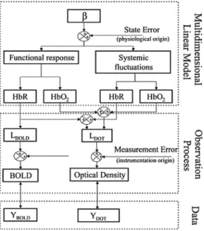
prin-ciples in the two modalities. These prinprin-ciples must be prop-erly considered to incorporate both MRI and optical datasets into a single model. In Fig.1, we present a schematic outline of our state model, which outlines how the measurement mod-els for both MRI and optical are connected to a common model of physiological contrast. The framework for this model is described by three components, which are described in the following sections: 1. a multidimensional linear model by which a set of spatial-temporal basis functions is used to describe functional and systemic components of oxy- and de-oxyhemoglobin concentration changes; 2. a set of measure-ment model equations describing the measuremeasure-ment biophysics for each modality and connecting the observations and under-lying physiology; and 3. the least-squares minimization rou-tine in which the experimental observations are fused to create a joint estimate of the underlying physiology.

2.3 Multidimensional Linear Model

To describe the underlying physiological changes within the brain, we assume that changes in oxy- and deoxyhemoglobin can be described as linear combinations of a set of spatial and temporal basis functions designated to capture the functional and physiological hemodynamic fluctuations. In principle, this approach is similar to the general linear model共GLM兲 which has been previously introduced for fMRI36,37and optical38,39 analysis, but has been modified here to include both spatial and temporal basis supports. Motivated by the anatomy of the brain and head and physiology of hemodynamic fluctuations, we introduced four distinct pairings of spatial and temporal

basis functions in our model. These groups were; 1. the func-tional brain elements共denoted as subscript “functional” or F兲, 2. a global brain physiology basis共subscript “brain global” or

B兲, 3. the cerebral spinal fluid 共CSF兲 layer surrounding the

brain共subscript CSF or C兲, and 4. the superficial skin layer 共subscript “skin” or S兲. These four groups of spatial basis functions are diagrammed in Fig.2.

The first group of canonic functions representing the indi-vidual functional brain elements was derived from a spatial basis set composed of overlapping Gaussian spheres posi-tioned on a hexagonal grid共as shown in Fig.2兲. This basis is

equivalent to a spatial smoothing kernel and is used in place of a separate smoothing operation applied to the data, as is usually typical of fMRI analysis. This basis also serves to reduce the unknown degrees of freedom of the model and makes the model more computationally tractable. We used a 6-mm standard deviation Gaussian kernel, which generated between 200 and 250 independent spatial functions 共depend-ing on the exact anatomy of the subject’s brain兲. These basis functions are restricted to those voxels that had been identi-fied as either gray or white cortical matter by a tissue segmen-tation algorithm using the MRI anatomical images共see Meth-ods in Sec. 3兲. The Gaussian spatial kernels were truncated at the anatomical boundaries between the brain and the CSF layers to impose a cortical constraint on the reconstruction of functional activation. The basis functions and reconstructions were limited to the contralateral hemisphere共opposite to hand movement兲 where optical measurements were recorded. The matrices representing each of the four types of spatial basis sets共denoted G in our model兲 have matrix dimensions of the number of independent basis functions共e.g., 200 to 250 for Fig. 1 Schematic outline of model. The multimodal fusion model is

based on a state-space approach and consists of three components. The set of coefficients to be estimated共␤兲 multiplies a convolution kernel of spatial and temporal basis functions in the multidimensional linear model to model the volumetric changes in oxy- and deoxyhe-moglobin due to evoked activation and systemic fluctuations. Linear observation models connect the underlying changes in these hemo-dynamic variables to expected measurements by both DOT and BOLD technologies. The states are finally estimated by minimizing the error with respect to the experimental data using a Bayesian for-mulation of the linear inversion operation.

Fig. 2 Basis functions in linear model. A set of spatial and temporal basis functions are used to regularize the model estimates of evoked and systemic hemodynamic changes. To model the different aspects of the physiology, four sets of basis sets are used. In the volume cor-responding to either gray or white brain matter, a gamma-variant func-tion共and derivative兲 was used as a temporal basis 共subplot C兲. These allow the modeling of the differing temporal dynamics of both oxy-and deoxyhemoglobin changes. A spatial basis of overlapping Gauss-ian spheres is used to reduce the dimensionality of the state space and replace a smoothing operation on the data共subplot B兲. To model the systemic contributions, the volume corresponding to skin, skull, and cerebral spinal fluid共CSF兲 layers are grouped into basis functions and given sine and cosine temporal functions to model their dynamics.

the functionally associated regions兲 by the number of voxels in the volume used for the optical and MRI forward models. When analyzing the experimental data, there are 28,672 col-umns in each of these matrixes 共the fMRI images had 64 ⫻64 in-plane resolution and seven axial slices兲. To model the temporal dynamics of evoked functional changes within each of these Gaussian bases, we used a linear combination of a two-parameter 共␴ and ␶兲 modified gamma function and its derivative共dispersion function兲, as given by the equations

t1共t兲 =共t −␶兲 2 ␴2_e−1 exp

冋

−共t −␶兲2 ␴2

册

, and t2共t兲 = 2 e−1

冋

冉

t −␶ ␴

冊

−

冉

t −␶ ␴

冊

3

册

· exp

冋

−共t −␶兲 2 ␴2

册

. 共1兲 The canonic temporal support vectors共t1and t2兲 are generated from the evaluation of these respective continuous-time func-tions关Eq.共1兲兴 at the discrete time points spanning the hemo-dynamic response共0 to 20 s at 2 Hz兲. This basis support is similar to the temporal basis often used in GLM analysis共e.g., the analysis of functional neuroimages共AFNI兲40or statistical parametric mapping 共SPM兲41 software packages兲. Since the temporal dynamics of the oxy- and deoxyhemoglobin re-sponses are known to differ, we used separate timing param-eters共␴and␶兲 for each hemoglobin species and denote these with subscriptHbO2and HbR, respectively. These timing pa-rameters were empirically estimated by a nonlinear fit to the group average of the region-of-interest average of the DOT time courses as a preprocessing step of this analysis. The em-pirical values of ␶ and ␴ used in the model were 共0.1 s⫾0.4 s, 6.7 s⫾0.3 s兲 and 共1.8 s⫾0.4 s, 6.7 s⫾0.3 s兲 for oxy- and deoxyhemoglobin, respectively共standard errors estimated from the five individual subjects兲. We note that the inclusion of the second dispersion support in the linear model allows for sufficient flexibility in the temporal shape of the estimated response to model each of the individual subject’s data, as demonstrated in previous MRI studies共e.g., Ref.42兲.

For example, in this study, we found that a linear combination of these two temporal functions can account for most of the evoked responses in each of five subjects 共R2_兩HbO2

= 0.81⫾0.08 and R2_{兩HbR=0.86⫾0.03; p⬍0.001 for all;} for the average of fivesubjects⫾StdErr兲.

The overall temporal model of the functional component of the hemodynamic signals can be expressed as the convolu-tion of the experimental stimulus timing 共U兲 and the func-tional impulse response functions 关t1 and t₂ in Eq. 共1兲 for either oxy- or deoxyhemoglobin兴:

TFunctional,HbO₂=

冋

t1,HbO₂ t2,HbO₂

册

丢U and TFunctional,HbR =

冋

t1,HbR t2,HbR

册

丢U, 共2兲

where U is the binary vector describing the experimental paradigm共i.e., the timing of stimulus presentation兲 and spans the temporal duration of the experiment. The dimensions of the T matrix are the number temporal basis functions by the number of measurement time points.

In addition to the first pairing of spatial-temporal basis functions, which is used to model the evoked functional re-sponse, the global brain, CSF, and skin groups of temporal basis functions are used as systemic regressors of background physiology. These were included to model nuisance physi-ological contributions to the BOLD and/or DOT measure-ments by using larger 共“super-voxel”兲 representations of the brain, CSF, and skin layers, as described in Fig.2and similar to the methods previously introduced to model systemic con-tributions to DOT signals.43For each of these basis groups, we paired the spatial basis with a series of sine and cosine functions 共1/20 to 1.0 Hz in 1/20-Hz steps兲 to describe the temporally oscillating systemic physiology. The skin-confined basis group models the systemic contributions to predomi-nantly the optical signals and the brain-confined nuisance re-gressor models physiology common to both modalities.

In total, the set of all spatial-temporal bases is combined into a single convolution operator 共GT兲, giving a total of eight unique basis groups 共four groups for both HbO2 and HbR兲. This matrix is formed by the convolution of the indi-vidual spatial 共G兲 and temporal 共T兲 basis functions at each time instance for each of the eight groups. The matrix GT is given by the equation:

GT =

冋

共GF,HbO2丢TF,HbO2兲 共GB,HbO2丢TB,HbO2兲 共GC,HbO2丢TC,HbO2兲 共GS,HbO2丢TS,HbO2兲

共GF,HbR丢TF,HbR兲 共GB,HbR丢TB,HbR兲 共GC,HbR丢TC,HbR兲 共GS,HbR丢TS,HbR兲

册

, 共3兲

where the subscripts F, B, C, and S indicate the functional, global brain, CSF, and skin basis groups. The matrix GT has dimensions of twice the number of image reconstruction vox-els multiplied by the number of discrete measurement time points 共rows兲 by the total number of model unknowns 共col-umns兲. The total number of model unknowns is equal to the number of spatial basis functions times the number of

tempo-ral basis functions and summed over the four tissue classifi-cations and two hemoglobin species. For example, in our 6 min of experimental data, the GT matrix is approximately 41,000⫻3000 elements, which would be 200 gigabytes in size for 16-bit numerical precision. Fortunately, in practice, this full matrix never needs to be stored in memory, because in the inverse problem we only need the inner product of two

such matrices共i.e., GTT_{GT兲, and this can be built up on a per}

time-point basis by making use of the block structure of this matrix and simple matrix operations. The details of this pro-cedure are not discussed in this work.

The basis function matrix 共GT兲 describes the spatial-temporal supports for the image reconstruction. Following the standard notation used previously to describe the general lin-ear model in fMRI analysis 共i.e., Ref. 44兲, the spatial and

temporal dynamics of the underlying hemoglobin changes are described by a linear sum of the spatial-temporal basis func-tion weighted by a vector of unknown coefficients denoted␤. The vector containing the modeled hemoglobin changes共both systemic and evoked兲 at each volume element and time point is thus given by the equation:

冤

⌬HbO2兩1 ] ⌬HbO2兩k ⌬HbR1 ] ⌬HbRk

冥

=

冋

⌬HbO2 ⌬HbR

册

= GT ·␤, 共4兲

where k is the total number of imaging parameters in the model and is equal to the number of time points multiplied by the number of volume elements. This matrix is a vectorized form of the reconstructed image共including time dimension兲 and is reshaped to a volumetric matrix in final analysis before displaying the images/movies.

2.4 Observation Models

The second component of our fusion model共as shown in Fig.

1兲 incorporates the measurement processes that relate the

un-derlying physiological changes 关oxy- and deoxyhemoglobin given by Eq. 共4兲兴 to the observations of each modality. The measurement equations for DOT and fMRI describe the bio-physics of each instrument measurement. In this work, we have approximated this biophysics using linear approxima-tions to these measurement equaapproxima-tions. The validity of these linear simplifications has been discussed by a number of re-searchers that have examined the consistency of these DOT and fMRI modalities with these hypothesized underlying bio-physical theories by correlating the temporal 共reviewed in Ref.10兲 and spatial45–47components of measurements. These works have suggested that linearity between the change in deoxyhemoglobin and the BOLD signal can be justified. Note that although our current model has been formulated using these linear approximations, nonlinear extensions of both the optical and fMRI models are theoretically possible using simi-lar methodologies共although the size of the model and com-putational memory requirements may currently limit this implementation in practice兲.

2.4.1 Blood oxygen level dependent measurement

model

The BOLD signal has a complex origin arising from both intra- and extravascular tissue.4,48,49These signals depend on not only the user acquisition parameters, such as echo time, magnetic field strength, and imaging echo type, but on fea-tures of the subject anatomy as well, such as vascular

archi-tecture and the orientation between blood vessels and the im-aging fields.50 In this work, we simplify the BOLD measurement model by considering only the extravascular 共EV兲 signal contribution. The EV signal is believed to com-pose the majority component of the BOLD signal at the 3 tesla共T兲 field strength.49The EV signal is linear to changes in the concentration of deoxyhemoglobin per volume tissue and is given by the equation4,48,51

⌬S共t兲 S0 = BOLD共t兲 ⬇ − 4.3 ·␷o· Vo· Eo· TE · ⌬关HbR共t兲兴 关HbR0兴 , 共5兲 where Vois the frequency offset in hertz of water at the outer

surface of a magnetized vessel共=80.6 s−1_{at3 T}52_{兲. E}

ois the

resting oxygen extraction fraction, and Vo is the baseline

blood volume to tissue fraction. TE is the echo time used in the MR pulse sequence 共30 ms in this study兲.关HbR0兴 is the baseline deoxyhemoglobin concentration. In general, the co-efficients of this equation are not known with the certainty required for quantitative imaging, and moreover, may vary between subjects according to the baseline state or spatial region.53 For this reason, empirically calibrated fMRI tech-niques have been proposed to remove the influences of these parameters by using ratios of the blood flow and oxygen satu-ration共i.e., BOLD兲 signals.12

To account for these unknown calibration parameters in the BOLD measurement equation, these factors are lumped into a single parameter 共␣⬅−4.3·␷o· Vo· Eo· TE/关HbR0兴兲. In our

method, we use the information in the optical data to help determine the BOLD calibration factor, as we describe in Methods in Sec. 3. In our measurement model, the BOLD signal is a projection of the deoxyhemoglobin component of the model plus an additive noise term共vBOLD兲 by the equation

YBOLD共t兲 = 关0␣· I兴 ·

再

⌬关HbO2共t兲兴

⌬关HbR共t兲兴

冎

+␷BOLD共t兲. 共6兲

2.4.2 Diffuse optical tomography measurement

model

In the DOT technique, near-infrared light is introduced into the head and propagates through the dense scattering layers of the scalp and skull into the brain. A small fraction of the light introduced eventually exits the head and is recorded a dis-tance away from the source position. Hemodynamic changes in oxy- and deoxyhemoglobin concentrations affect the ab-sorption properties of the brain and thus result in changes in the intensity of light as it migrates along a diffuse trajectory through the head. Using multiple measurements taken by an array of light source and detector positions spaced several centimeters apart共shown in Fig.3兲, the DOT method can be

used to spatially resolve these absorption changes and relate these to changes in oxy- and deoxyhemoglobin. The DOT measurement equation is described by the spatial profile of the light propagation through the head, which determines the sensitivity of these measurements. To derive the distribution of photons in a medium with a complex distribution of ab-sorption and reduced scattering coefficients关␮a共r兲 and␮s

⬘

共r兲,

must be modeled by empirical means using computerized simulations. In Monte-Carlo-based modeling, the distribution of these photons is statistically modeled based on the prob-ability of an absorption or scattering event at each region of space as described by␮a共r兲 and␮s

⬘

共r兲.

54,55

For brain activation, the changes in the optical properties are generally small共on the order of a few percent兲, and thus,

a linear approximation is believed to be sufficient for predict-ing the changes in optical measurements produced by local-ized changes in the optical properties共reviewed in Ref.23兲.

The spectroscopic forward model for such optical measure-ments is of the form56–58

冋

Y_DOT830 nm共t兲 Y_DOT690 nm共t兲

册

=

冋

␧HbO830 nm_{2 · A}830 nm ␧HbR830 nm · A830 nm ␧HbO690 nm_{2 · A}690 nm ␧HbR690 nm · A690 nm

册

·

再

⌬关HbO2共t兲兴 ⌬关HbR共t兲兴

冎

+

冋

␷DOT 830 nm_共t兲 ␷DOT 690 nm_共t兲

册

, 共7兲

where Y is the vector of measured optical signal changes for each source-detector pair and A␭is a matrix describing the linear projection from absorption changes from within the volume to optical signal changes between each measurement pair. ␭ indicates wavelength dependence 共690- and 830-nm wavelengths were used in this study兲. Each row of the matrix

A describes the light propagation between a particular optical

source and detector pair 共shown in Fig.3兲, which describes

the spatial sensitivity for that measurement. The A␭matrix is a projection operator, which integrates absorption changes over the volume to predict the measurements between sources and detectors. It has been shown that this linear operator is approximated by the adjunct product between the photon den-sity distributions for each given source and each given detec-tor involved in each optical measurement.7 In Eq. 共6兲, the

projection operators are combined with the spectral extinction coefficients共␧␭兲 to give a direct forward operator between the concentration changes in HbO2 and HbR 共per volume ele-ment兲 and the measured optical density changes at multiple wavelengths. In our model, v␭ is an additive measurement noise term specific to each measurement channel and wave-length.

2.5 Data Fusion Model

Rather than treating the DOT and BOLD measurements inde-pendently or first computing an MR-based spatial map to be used as a reconstruction prior, our model tries to preserve the mutual information in the multimodal data by simultaneously considering measurements from both instruments. We concat-enate the two measurement equations关Eqs.共6兲and共7兲兴 into a single joint-observation operator

L =

冤

␧HbO830 nm_{2 · A}830 nm ␧HbR830 nm_{· A}830 nm ␧HbO690 nm₂ · A690 nm _␧HbR690 nm_{· A}690 nm 0 ␣· I

冥

. 共8兲

The joint set of multimodal data can be expressed as the mul-tiplication of the underlying model of oxy- and deoxyhemo-globin changes by the linear observation operator. Combining Eqs.共4兲and共8兲, the complete model equation can be written as

冤

Y_DOT830 nm Y_DOT690 nm YBOLD

冥

=共L丢In兲 · GT ·␤+

冤

␷DOT 830 nm ␷DOT 690 nm ␷BOLD

冥

, 共9兲

where Inis an identity matrix with size equal to the number of

measured time points共n兲. The total model considers both time and space simultaneously共as defined by the spatial and tem-poral basis matrix GT兲. This final model can be written as a single matrix equation,

Y = L ·共GT ·␤兲 +␷, 共10兲 where Y has dimensions of total number of measurements 共number of optical plus MRI measurements for all time Fig. 3 Diffuse optical tomography. Diffuse optical tomography uses

spectroscopic measurements of optical absorption changes to record hemoglobin concentration changes.共a兲 The optical probe was placed over the subject’s primary motor area.共d兲 The probe contained four source and eight detector positions spaced 2.9 cm apart.共b兲 and 共c兲 Fiducial markers on the probe were visible in the anatomical MR images.共e兲 The position of the probe and a segmented layer model for each subject were used to generate the optical sensitivity profiles us-ing Monte Carlo methods.

points兲 and can be written by concatenating the set of mea-surements for all time points共t苸关1 n兴兲 as

Y =关y1Ty₂T _{¯ yn}T兴T. 共11兲 Similarly, the measurement model matrix L must be extended by replicating this matrix along the diagonal for each of the measurement time points. In our experimental data, both op-tical and MRI data have the same sample rate共2 Hz兲 and thus all discrete observation points use the same joint measurement equation, which includes both optical and fMRI measurement models. However, in general, the fMRI acquisition rate will be considerably slower than that of the DOT, and this can be accounted for in our model by time indexing the measurement operator共L兲 to use observations for one or both of the appro-priate modalities at each observation point, depending on the samples acquired at that time. Thus, this model can be used to interpolate the reconstructed image using the higher temporal resolution DOT data, while maintaining a solution that is less frequently spatially constrained by fMRI measurements.

2.6 Bayesian Inversion Routine

To estimate the coefficients for the spatial-temporal basis sets describing changes inHbO2and HbR, the linear model关Eq.

共10兲兴 is solved using a Bayesian formulation of the linear inverse operator59

␤ˆ = 共HT_{· R}−1_{· H +⌫}2_{· O}−1_兲−1_{· H}T_{· R}−1_{· Y. 共12兲} In Eq.共12兲, R−1 _and⌫2_Q−1 _{represent the inverses of the} covariance for the observation noise and state noise models, respectively. We have chosen this formulation over the Tikhonov regularization共Moore-Penrose generalized inverse兲, which is more commonly used in DOT, because the Bayesian formulation separates the regularization parameters into both an observation noise共R−1_{兲 and a state noise 共⌫}2_Q−1_兲 precon-ditioning term. A similar regularized inverse scheme was re-cently described by Yalavarthy et al.60This weighted least-squares method provides a better framework to introduce differential observation noise for each modality. From a sta-tistical standpoint,⌫2Q−1_{is a covariance prior on the states␤.} This definition offers some intuitive guidance on how to tune the inversion, since we expect physiological fluctuations to be approximately on the order of micromolar magnitudes. In practice, however, the multidimensional linear model is only an approximation of the actual physical system, and the as-sumed Gaussian distributed prior on ␤ is imperfect. These approximations effectively mean that the Bayesian inverse is a regularization scheme that must be tuned, and we have in-troduced a scalar parameter ⌫ for that purpose. In addition, we define the variance of the observation 共measurement兲 noise model共␷兲 as a diagonal matrix formed from the vari-ance关var共 兲兴 of each measurement, i.e.,

R =

冤

var共␷DOT 830 nm_{兲 0 0} 0 var共␷_DOT690 nm兲 0 0 0 var共␷BOLD兲

冥

. 共13兲

Thus, the measurement noise covariance can be estimated from experimental data and is used to reflect our confidence in the measurements taken from the two different modalities as a

statistical prior, as described in Methods in Sec. 3. In this model, we have assumed that both the process and the mea-surement error for each modality are zero-mean random vari-ables.

3 Methods

3.1 Experimental Methods

The experimental protocol used in this study has been previ-ously described.61The data used in this analysis have been previously reported in that paper for comparison of the tem-poral characteristics of optical methods and fMRI. Five healthy, right-handed subjects共4 male, 1 female兲 were imaged in this experiment. The task consisted of a two-second dura-tion finger-walking on the right共dominant兲 hand. The Institu-tional Review Board at Massachusetts General Hospital ap-proved these procedures.

3.2 Diffuse Optical Tomography Acquisition and

Preprocessing

We used a multichannel continuous-wave optical imager 共CW4, TechEn Incorporated, Milford, Massachusetts兲 to ob-tain the measurements as previously described.62 The DOT imager has 18 lasers—nine lasers at 690 nm 共18 mW兲 and nine at 830 nm 共7 mW兲—and 16 detectors of which only four source positions and eight detectors were used here. The laser wavelengths were 690 and830 nm共18 and 7 mW, re-spectively兲.

The DOT probe was made from flexible plastic strips with plastic caps inserted in it to hold the ends of the 10-m-source/detector fiber optic bundles. The probe consisted of two rows of four detector fibers, and one row of four source fibers arranged in a rectangular grid pattern and spaced 2.9 cm between nearest neighbor source-detector pairs 共shown in Fig.3兲. This plastic probe was then secured to the

subject’s head centered over the contralateral primary motor cortex共M1兲 via Velcro straps and foam padding. The 10-m fibers were run through the magnet bore to the back of the scanner and through a port into the control room, where they were connected to the DOT instrument.

Following collection and separation of source-detector pairs, the timing of the DOT data was synchronized to the MRI images共as described in Ref.61兲. The data were

down-sampled using a Nyquist filter to the same2-Hz sample fre-quency as the fMRI. The raw light fluence measurements were converted to changes in optical density by the negative log of the normalized incident light intensity 兵⌬OD␭共t兲 = −log关I␭_共t兲/I␭_{共0兲兴其.}

Monte Carlo methods were used to generate the optical sensitivity profiles describing the DOT measurement equation 关Eq.共6兲兴.45,55,63

Anatomical MP-RAGE images acquired dur-ing the session were segmented into a five-layered head model for each of the subjects,45 which was used for these Monte Carlo simulations and also to define the spatial basis functions used in the linear model. From the vitamin E fidu-cial markers used to mark the optical probe, the locations of the DOT optodes were located. The photon migration paths were sampled from the simulated trajectories of108 _photons at both 690- and 830-nm wavelengths. These simulations were used to calculate the linear optical forward matrices

共A␭_{兲 and substituted into Eq. 共7兲共see Fig.3兲. To create the} spectroscopic forward operator, the hemoglobin extinction co-efficients were used from the Oregon Medical Laser Center 共http://omlc.ogi.edu/兲.

3.3 Functional Magnetic Resonance Imaging

Acquisition and Preprocessing

BOLD-fMRI measurements were performed using a 3 tesla Allegra scanner 共Siemens Medical Systems, Erlangen Germany兲. fMRI data were collected using a gradient echo

planar imaging 共EPI兲 sequence 关TR/TE/␣

= 500 ms/30 ms/90 deg兴 with seven 5-mm oblique orienta-tion slices共1-mm spacing兲 and 3.75-mm in-plane spatial res-olution. Structural scans were performed using a T1-weighted

MPRAGE sequence 共1⫻1⫻1.33-mm resolution,

TR/TI/TE/␣= 2530 ms/1100 ms/3.25 ms/7 deg兴. The BOLD time series was preprocessed using a motion-correction algorithm64 and mean normalized before being used in the model.

3.4 Numerical Simulations

We used simulation studies to test the quantitative accuracy of this method. This enables us to examine the ability to quantify hemoglobin changes, since no empirical “gold-standard” method exists that can provide quantitative measurements with which to validate our experimental results. Simulated inclusions were placed shallow 共⬃18 mm兲 and deep 共⬃25 mm兲 from the surface of the head 共shown in Fig.4兲.

The hemodynamic response was simulated with a maximum peak value of8␮M and −2.5␮M for oxy- and deoxyhemo-globin concentration changes, respectively. Varied levels of measurement noise were added to the simulated measure-ments to create varied levels of contrast-to-noise ratios.

3.5 Optical Calibration of the Blood Oxygen Level

Dependent Signal

The BOLD measurement model depends on an unknown cali-bration factor 共␣兲, which depicts the several baseline and structural unknown factors within Eq. 共5兲. This calibration factor is determined empirically by comparing the spatial and temporal profiles of the DOT and BOLD data as described in Ref. 45. Using the linear forward operator describing the DOT measurement model关Eq.共7兲兴, we project the model es-timate of the BOLD signal from its natural volume space representation into the optical measurement 共i.e., source-detector兲 space. By substituting Eq. 共6兲into Eq. 共7兲, the ex-pected optical signals due to a change in deoxyhemoglobin can be modeled from the model estimated BOLD signal, as discussed in Ref.45.

冋

⌬ODBOLD830 nm_共␣兲 ⌬ODBOLD690 nm_共␣兲

册

=

冋

␧HbO2 830 nm_{· A}830 nm ␧HbR830 nm · A830 nm ␧HbO690 nm_{2 · A}690 nm ␧HbR690 nm_{· A}690 nm

册

·

冋

0 YˆBOLD/␣

册

. 共14兲

These BOLD derived multiwavelength optical density changes can be used to estimate the change in deoxyhemoglo-bin predicted by the spatial location and magnitude of the BOLD signal共⌬关HbR兴BOLD兲 for each source-detector pair us-ing the modified Beer-Lambert law,65,66and compared to the measured optical data to find the calibration factor共␣兲 using the equation

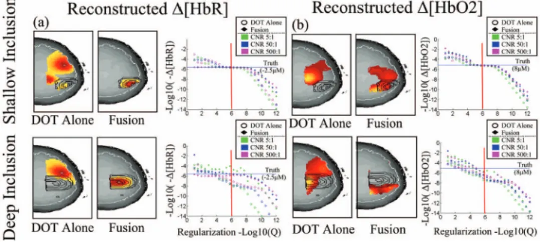
Fig. 4 Characterization of model quantitative accuracy. The quantitative accuracy of the model was examined with observations simulated from a shallow共18 mm, toprow兲 and deep 共25 mm, bottomrow兲 inclusion. The simulated inclusions are shown contoured 共black兲 in each image 共axial projections兲. The boundaries of the cortex are outlined in white. Measurement noise was added to achieve a 5:1, 50:1, and 500:1 contrast-to-noise ratio共CNR兲. Hemoglobin changes were reconstructed using the fusion model and DOT data alone for comparison. Reconstructions were per-formed at various regularization amounts to examine the dependence of the recovered magnitude of the response on the regularization parameter. The images are shown for the reconstruction at 1 /⌫=1␮M共indicated by the vertical red line兲 for the CNR=50:1 case.

⌬关HbR兴BOLDsource-detector_{共␣兲 =}␧HbR 830 nm_·⌬ODBOLD830 nm_{共␣兲/共L · DPF}830 nm_{兲 − ␧HbR}690 nm_·⌬ODBOLD690 nm_{共␣兲/共L · DPF}690 nm_兲 ␧HbR830 nm_·␧HbO 2 690 nm_−␧HbR690 nm_·␧HbO 2 830 nm , ␣= arg min ␣ 兩⌬关HˆbR兴DOT

source-detector_{−⌬关HbR共␣兲兴BOLD}source-detector_{兩. 共15兲}

In the modified Beer-Lambert equation关top in Eq.共15兲兴, L is the linear distance between the position of a source and detector, and DPF is the differential path-length factor, which is a dimensionless coefficient defined as the effective path length through the head divided by the source-detector separation.63,65,66 This is calculated from the Monte Carlo simulations. Since this projection uses the optical forward model, it accounts for the DOT partial volume errors in the calibration of the BOLD signal. A single calibration factor共␣兲 was used, which is consistent with findings of the spatial cor-relation of response amplitudes between the two modalities.45,46 To estimate this parameter in the model, we employ an iteration routine between state and parameter esti-mation. Alpha共␣兲 is first estimated via Eq.共15兲using the raw optical and MRI data, and then the states 共␤兲 are estimated using Eq.共12兲. The estimated optical and BOLD signals are recovered from the forward model using the estimated value of beta, and the alpha is re-estimated from the modeled BOLD and optical signals using the bottom of Eq.共15兲. This beta and alpha estimation process was repeated for 20 itera-tions. Alpha was found to converge below a+/−10% varia-tion after a few iteravaria-tions共approximately five iterations兲.

3.6 Estimation of Noise Covariance

To estimate the covariance of the measurement noise共R兲, we calculated the variance of the residual for each measurement by iteratively solving the state estimate and estimating R to be the variance of the residual of the measurements. The initial seed of R was calculated from linear regression of the data with the temporal basis.

An identity matrix was used for the state covariance matrix

Q. The regularization tuning parameter共⌫兲 was adjusted in

the analysis, as noted in Sec. 4. A single regularization param-eter was used to scale the variance of both the oxy- and de-oxyhemoglobin states.

4 Results

4.1 Simulation Studies

To investigate the improvements in the reconstruction accu-racy, forward simulations of synthetic data and inverse recon-structions were first performed as described in Sec. 3. The simulated observation vectors were reconstructed using the DOT only and the multimodal fusion共DOT and BOLD兲 data in the reconstructions. Reconstructed axial slices are shown in Fig.4 for the shallow and deep simulated inclusions. Using only the DOT data, the image reconstruction of both oxy- and deoxyhemoglobin depend strongly on the regularization pa-rameter used共⌫兲. In Fig.4, reconstructions are represented at regularization values of 1/⌫=共1␮M兲. To examine the

de-pendence of the reconstruction accuracy on the regularization parameter, we looked at the reconstructed response amplitude and goodness-of-fit of the model for varied levels of regular-ization. This was repeated for both the shallow and deep in-clusions and at several levels of simulated instrument noise 共5:1, 50:1, or 500:1 contrast-to-noise ratio兲. The results, shown in Fig. 4, demonstrate the robustness of the fusion model to the choice of this regularization for deoxyhemoglo-bin reconstructions. Since the estimate of deoxyhemoglodeoxyhemoglo-bin change is overdetermined in the presence of both optical and BOLD measurements, accurate estimates of the response are recovered at minimal regularization. When over-regularization is applied, the response is underestimated, as expected. In contrast, reconstructions using only the DOT data show high dependence on the regularization amount. This result is consistent with prior expectations of the behav-ior of the DOT inverse problem with our measurement geom-etry. The fusion reconstruction of oxyhemoglobin changes is also dependent on the regularization applied. This is due to the fact that the reconstruction of oxyhemoglobin changes is only indirectly informed by the fMRI data through the off-diagonal terms in the spectroscopic optical forward model 关Eq. 共7兲兴. Since only the DOT measurements contain direct information about oxyhemoglobin, this component of the in-verse problem is still ill posed and requires significant regu-larization. However, the oxyhemoglobin reconstructions are still modestly improved by the fusion reconstruction over the DOT-only reconstruction.

4.2 Experimental Studies

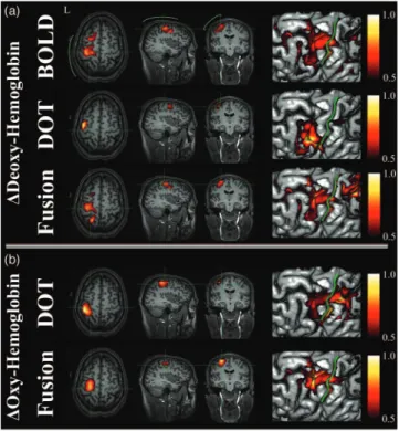
Images of evoked hemoglobin changes were reconstructed from the BOLD alone, DOT alone, and multimodal 共fusion兲 experimental datasets for all five subjects, as shown in Figs.5

and6. In Fig.5, we show an in-depth look at the results for a single subject 共subject A兲, and show the reconstructions of deoxyhemoglobin共upper rows兲 and oxyhemoglobin 共bottom rows兲. The right column of images in Fig.5shows the surface rendering of the activation regions with the central sulcus marked for clarification. In Fig.6, we show the reconstructed results for the data-fusion method for subjects B through E and comparison to the BOLD model. In agreement with pre-vious analysis of this data,61 we found localized functional activation in the motor-cortex共M1; precentral gyrus兲 and pri-mary sensory共S1; post-central gyrus兲 regions for each of the individual five subjects for the fMRI and fusion reconstruc-tions. The peak amplitudes of the estimated evoked oxy- and deoxyhemoglobin responses are given in Table1. In general, the multimodal fusion and BOLD images were similar, al-though a few notable differences were observed. These differ-ences are most likely the result of differdiffer-ences in the

regular-ization in the two models. A regularregular-ization amount共1/⌫兲 of 10␮M was used in the DOT and fusion reconstructions, and 10% in the BOLD images, which may account for these dif-ferences. In addition, the fusion images are more sensitive than single modality methods to both temporal and spatial registration errors between the two modalities, which can in-clude intrinsic differences due to differential vascular sensi-tivity. This can introduce disinformation between modalities, which will result in the loss of confidence of an activation event and lower functional effects statistics共e.g., more likely to reject a null hypothesis兲.

In the model reconstructions that only used the DOT data, we found that the amplitudes of the estimated hemoglobin changes were dependent on the regularization applied, which was consistent with the simulation results and prior expecta-tions on the behavior of the ill-posed inversion of the optical forward model and minimum norm estimator. The reconstruc-tions shown in Figs.5and6and values given in Table1were obtained at a regularization value of1/⌫=10␮M, which pro-vided the best reconstruction from the optical data alone when qualitatively compared to the fusion or BOLD reconstruc-tions. We have chosen to present images using this regular-ization point to give the best possible representation of optical-only reconstructions for comparison to the data fusion method. With this choice of regularization, the optical-only results were qualitatively close to the fMRI images共as dem-onstrated in Fig.5for subject A兲, although distinct biases in the spatial locations were notable. Even with the cortical con-straint of our model, we noted that our optical-only recon-structions tended to be biased toward the locations of optodes, which, in most cases, displaced the location of the DOT re-constructions relative to the BOLD alone or fusion derived estimates. In contrast to the deoxyhemoglobin reconstruc-tions, the improvements of the fusion model to estimate of oxyhemoglobin changes over the DOT alone model were less dramatic. However, we found that the fusion estimates of oxy-hemoglobin were less susceptible to biases toward the optode positions, although they were still superficially biased toward the head’s surface. The optical probe used in this study was based on a simple nearest-neighbor geometry. Recent work has shown that optical-only reconstructions could be further improved using tomographic probe designs, including the use of overlapping measurements 共e.g., Refs.24 and 25兲. These

methods would be expected to further improve the accuracy of the reconstructions performed here for both optical-only and fusion methods.

In addition to the functionally evoked responses, our model also includes regressors for the background physiologi-cal oscillations modeled as global effects using large spatial basis supports. The inclusion of these regressors accounted for an average of an additional8.5%⫾4.4% of the total model variance based on partial R2analysis of the model共average of fivesubjects⫾StdErr; range 3.3%关subject B兴 to 26.3%关sub-ject E兴兲. As recently demonstrate by Diamond et al.43using optical measurements and Glover, Li, and Ress67using fMRI measurements, the use of direct measurements of systemic physiology by pulse-oximtery or noninvasive blood pressure methods as additional model regressors may provide further reduction of these cerebral physiological signals and should be examined in future work.

Fig. 5 Direct hemoglobin reconstructions from empirical data. This figure shows 共b兲 the model reconstructions using the DOT alone, BOLD alone, and共a兲 fusion datasets for deoxy- and oxyhemoglobin changes. Data are represented for subject A. All responses have been normalized for comparison. Reconstructions were performed at a regularization level of 1 /⌫=10␮M for the DOT and fusion models and 1 /⌫=10% for the BOLD model. Functional changes are shown masked below the half-max response amplitude. In共a兲 the approxi-mate location of the optical probe is shown in green. The right-most images show the maximum intensity projections of the activation pat-terns onto the brain pial surface关surfaces generated using Freesurfer 共The Massachusetts General Hospital; see http// surfer.nmr.mgh.harvard.edu兲兴 and displayed using NeuroLens 关Univer-sité de Montréal;共see http://www.neurolens.org兲兴. The central sulcus is outlined共green line兲 in each surface image.

Fig. 6 Comparison of fusion and MRI image reconstructions. In this figure, we show the BOLD共a兲 and fusion reconstructions 共b兲 for sub-jects B through E共left to right兲. Subject A was presented in Fig. 5. Regularization was applied as described for Fig. 5. All images are shown normalized to the maximum response and masked below the half-max amplitude. Axial and coronal projections are shown. The outline of the boundary between the brain and superficial layers is shown in green. The blue rectangle indicates the location of the im-aging volume from the fMRI.

4.3 Optical Calibration of Blood Oxygenation Level

Dependent

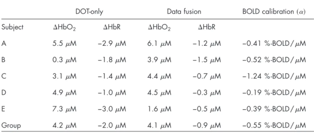
In Table 1, we show the recovered values of the optically calibrated BOLD scaling factor共␣兲 for each of the five sub-jects 共mean: −0.55%-BOLD/␮M⫾0.40%-BOLD/␮M兲. The high variance in the group estimate may be the result of differences in the baseline volume or oxygen extraction levels between subjects共particularly subject C兲. In addition, the val-ues of the BOLD model parameters given in Eq.共5兲are based on additional assumptions about the size and orientation of blood vessels共i.e., Ref. 50兲 and may also contribute to the

differences observed between the five subjects. We can com-pare our measured values of alpha with theoretical estimates derived from Eq.共4兲 and data from previous literature. As-suming a baseline blood volume fraction of 3 to 5%,68,69 a total hemoglobin concentration of 60 to 100␮M,70 and an oxygen extraction fraction of 30 to 40%,69,71 the expected value for this calibration factor can be estimated to be be-tween−0.3 to − 0.9% -BOLD/␮M--HbR for the MRI acqui-sition parameters used in this study. This calibration factor has also been determined experimentally by the hypercapnia method of BOLD calibration described by Davis et al.12The hypercapnia calibration method determines the maximal BOLD change possible if all deoxyhemoglobin were dis-placed from the region共reviewed in Ref.19兲. Thus, according

to our approximation of a primarily extravascular water con-tribution to the BOLD signal, as given by Eq.共5兲, this hyper-capnia calibration factor共usually denoted M兲 can be related to our alpha parameter by multiplying by the baseline deoxyhe-moglobin levels共i.e., M⬇␣⫻关HbR0兴兲. The empirical value of M has been reported between 7 to 25% as tabulated in Ref.

19, which corresponds to a value of alpha between−0.4 and −1.4% -BOLD/␮M using the ranges of baseline total hemo-globin and oxygen extraction cited before. Indeed, both the empirical and theoretical estimates of this calibration factor are consistent with our values calculated for the five subjects, as shown in Table1. In future work, it will be necessary to validate the optical-calibration approach against other calibra-tion methods like the hypercapnic method.

5 Discussion

Concurrent multimodal measurements are observations of common underlying changes in underlying functional con-trast. Our fusion model combines this mutual information from optical and fMRI modalities into a joint estimate of un-derlying hemoglobin changes. This approach provides a framework to combine the advantages of the high spatial and temporal resolutions contained between both modalities. In this work, we have developed a model that incorporates the biophysical principles that describe the relationships between the optical and fMRI measurements and underlying cerebral physiology. Using a single image reconstruction step, we can obtain direct estimates of hemoglobin changes that are simul-taneously consistent with all sets of observations. This allows us to use the high spatial resolution of fMRI as a spatial prior to improve the optical reconstruction, while at the same time, to use high temporal and spectroscopic information from the DOT as priors on the reconstruction of the BOLD functional changes. The fusion of the higher spatial information from fMRI measurements and the spectroscopic information of the optical technique provided cross-calibrated estimates of he-moglobin changes. The Bayesian framework used in this model allows us to optimally incorporate data from different sensors based on knowledge of the statistical errors in each measurement type. In comparison to methods using fMRI as a statistical prior for the optical reconstruction, our approach incorporates multimodal information based on the statistical properties of concurrent measurements. We believe that this approach provides a framework to more efficiently consider concurrent multimodal datasets and to utilize the mutual in-formation in the signals to improve the accuracy of estimates of the functional response. The advantages of this approach have been discussed for data fusion of magnetoencephalogra-phy and electroencephalogramagnetoencephalogra-phy data using similar mutual in-formation models 共e.g., Refs. 34 and 35兲. We believe that

future extensions of our method will offer similar utilities for hemodynamic imaging.

Table 1 Comparison of reconstructed hemoglobin amplitudes. The maximum 共minimum兲 response amplitude was calculated for a region of interest in each of the DOT alone and fusion reconstructions for the five subjects. Regions of interest were manually defined in the motor cortex area. The BOLD cali-bration factor共␣兲 was calculated as described in the text. The values shown are for the reconstructions at a regularization 1 /⌫=10␮M.

DOT-only Data fusion BOLD calibration共␣兲

Subject ⌬HbO2 ⌬HbR ⌬HbO2 ⌬HbR

A 5.5␮M −2.9␮M 6.1␮M −1.2␮M −0.41 %-BOLD/␮M B 0.3␮M −1.8␮M 3.9␮M −1.5␮M −0.52 %-BOLD/␮M C 3.1␮M −1.4␮M 4.4␮M −0.7␮M −1.24 %-BOLD/␮M D 4.9␮M −1.0␮M 4.5␮M −0.3␮M −0.19 %-BOLD/␮M E 7.3␮M −3.0␮M 1.6␮M −0.5␮M −0.39 %-BOLD/␮M Group 4.2␮M −2.0␮M 4.1␮M −0.9␮M −0.55 %-BOLD/␮M

5.1 Comparison of Reconstruction Methods

In the comparisons between the optical only, BOLD only, and fusion reconstructions of the simulated data, we found that fusion methods produced the most accurate estimates of he-moglobin changes both in terms of spatial localization and quantitative accuracy. In particular, we found that for the fu-sion reconstructions of deoxyhemoglobin, the amplitude of these changes was relatively independent of the magnitude of the regularization applied and were fairly robust to errors in underestimation of the regularization parameter共⌫兲, as dem-onstrated in Fig.4. In the fusion model, enough information is available to make the deoxyhemoglobin reconstruction prob-lem overdetermined. Even at a minimal regularization level, the quantitatively accurate magnitudes of the deoxyhemoglo-bin responses were still recovered for both the deep and shal-low deoxyhemoglobin inclusions. As expected, an over-regularization of the linear model resulted in underestimation of the hemodynamic response in all models. In contrast to deoxyhemoglobin, which is directly informed by the BOLD model, we found that reconstructions of oxyhemoglobin changes in the fusion were still dependent on the regulariza-tion. This is because oxyhemoglobin is only indirectly in-formed by the BOLD signal and still represents an underde-termined problem.

In comparison, we found that our DOT alone model was generally more superficially biased than the fusion model at recovering the spatial profile of both targets, and that the am-plitude was very sensitive to the amount of regularization ap-plied. This bias will result in an underestimation of the re-sponse amplitudes, since the optical sensitivity profiles fall exponentially with increasing depth. This finding is consistent with prior expectations concerning the accuracy of DOT re-constructions. Although the spatial basis functions used in this work ensured a cortical constraint to functional activations, the reconstructed amplitudes were underestimated by up to several orders of magnitude, in particular for the deep simu-lated inclusion, and the magnitude of the DOT estimated he-moglobin changes were highly dependent on the regulariza-tion parameters used.

The DOT alone and fusion reconstructions of the empirical data were consistent with the findings from the simulations. The spatial locations of the fusion reconstructions were more consistent with the profiles from the BOLD alone. Although the magnitudes of the changes were comparable in our final images, the DOT reconstructions were highly dependent on the regularization applied, which was chosen here to provide the best possible DOT reconstructions based on the BOLD result. Thus, this may be misleading to the quality of the reconstructions that can be obtained routinely by DOT alone.

5.2 Optically Calibrated Blood Oxygen Level

Dependent Signals

In addition to the Bayesian fusion model that we have intro-duced in this work, we have also presented a method for using the spectroscopic information of the optical data to provide insight into the BOLD signal, allowing for optically calibrated BOLD imaging. In this work, we have assumed that a single calibration factor can be applied to calibrate the BOLD signal. In both the simulation and experimental results, we found that the estimate of this factor converged after only a few

itera-tions of the model. In the simulation results, we found that we could recover this calibration factor. In the experimental re-sults, we found approximate agreement between our estimates of this factor and the expectation from theoretical work ap-proximated at 3T and the empirical hypercapnia-based BOLD calibration.

5.3 Model Limitations and Future Extensions

While our data fusion method greatly improves the recon-struction and quantitative accuracy of deoxyhemoglobin changes, the improvements to oxyhemoglobin quantification were more modest. In principle, the state covariance matrix 共Q兲 used in the Bayesian pseudoinverse model 关Eq.共12兲兴 can be used to introduce a statistical prior between deoxy- and oxyhemoglobin maps with the inclusion of off-diagonal ele-ments connecting the two matrix quadrants for oxy- and de-oxyhemoglobin. However, in the work described here, we have purposefully not included these off-diagonal terms based on recent work that has suggested that underlying vascular structures may displace the locations of the two chromophores due to differential arterial versus venous weightings.45–47,72In support of this, several recent fMRI-based studies have also shown spatial displacements between the BOLD signal and MR measures of blood volume73and blood flow,74which cor-roborate a spatial displacement of arterial and venous-weighted measurements. In future studies, we suggest that the incorporation of an MR measure of blood volume changes73,75,76into this data fusion model may be more appro-priate to constrain total-hemoglobin changes and conse-quently the quantification of oxyhemoglobin.

An assumption made in this model was that we only ex-amined the extravascular contribution to the BOLD signal. This assumption ignores the contribution from the water mol-ecules within the blood vessels that interact directly with the deoxyhemoglobin heme group.1,4,48,77This assumption is sup-ported by recent work by Lu and van Zijl determined that the extravascular signal composes approximately 67% of the in-trinsic relaxation共⌬R

2

*_{兲 at 3 tesla.}49

Further evidence of the dominance of the extravascular signal has also been demon-strated in the empirical comparison of optical and BOLD sig-nals, which have shown a strong temporal correlation between the BOLD signal and the optical measure of deoxyhemoglo-bin 共reviewed by Ref.10兲. Thus, the source of BOLD

func-tional contrast at3 tesla is expected to be predominantly ex-travascular, which we believe justifies the assumption in this model in this current work. However, at lower field strengths, alternative MR acquisition protocols, or for more quantita-tively accurate results, the intravascular component may be-come necessary. The inclusion of the intervascular component of the fMRI signal creates a nonlinearity in the BOLD mea-surement equation, which additionally depends on changes in the venous blood volume that determine oxygen saturation changes共i.e., Ref.48兲. The future extension of this model to

incorporate this term can be achieved by the replacement of the linear 共extravascular BOLD兲 measurement model in Eq.

共5兲 with a more detailed state-space model of the vascular physiology共i.e., Refs.78–81兲. In future work, vascular

mod-els such as the Balloon77or Windkessel82models will enable the incorporation of more modalities into the model, such as blood flow.83 This nonlinear extension of this bottom-up