Diffusion of momentum and salinity in Lake Maracaibo, Venezuela

DIFFUSION OF

10MENTUT4 AND SALIHITY IN

LAKE MARACAIBO, VENIEZUELA

by

JOHN ROSS YEARSLEY

S.B., Massachusetts Institute of Technology (1958)

M.S., University of Washington (1966)

SUBMITTED IN PARTIAL FULFILLM1ENT OF THE REQUIREENTS FOR THE DEGREE OF MASTER OF SCIENCE

at the

MASSACHUSETTS INSITUI'E OF TECHNOLOGY May 1968

Signature of Auth6r. . . . , , " %-, , -. .-. . . . .. [Department oi Geologya Geophysics

A (May 23, 1968)

Certified by . . . . . . . . -,... .... *

C*/ Thesis Supervisor

Accepted by. . . . . , . . . . Chairman, Departmental Cormittee

on Graduate Studonts

Lindgren

WIT

(iqOM

1-6

inoAmlE

(ii)

ABSTRACT

DIFFUSION OF MOM101, UM AND SAL-ITfCY

IN

LAKE MARACAIBO, VENEZUELA

by

John Ross Yearsley

Submitted to the Department of Geology and Geophysics on May 23, 1968 in partial fulfillment of the requirements

for the degree of Master of Science

A theoretical model of the time-dependent motion in a

rotating stratified fluid, driven by a wind stress applied at the surface, is developed. Theoretical expressions for the radial, azimuthal and vertical velocities, and salinity are obtained.

The steady-state velocity and salinity profiles predicted

by the theory are compared to the results of a field survey

made in Lake Maracaibo by Redfield et al (1955). No data is available from Lake Mbaracaibo to verify the validity of the time-dependent portion of the theory, which predicts that

the velocity and salinity fields in the Lake require approximately 19 days to reach equilibrium a-fter a change in the applied wind

stress.

Thesis Supervisor: Arthur T. Ippen Title: Ford Professor of Engineering

(iii)

ACOTOWLEDGEIMITS

Financial support for this research was provided by a Ford Foundation grant to the Inter-American Project in the Department of Civil Eigineering, M.I.T.

Professor A. T. Ippen, who supervised the thesis, read the manuscript critically and offered numerous helpful suggestions

and criticisms.

Drs. Ralph H. Cross and Claes Rooth also read the manuscript and provided constructive criticism.

(iv) TABLE OF CONTENTS Page Abstract . . . . . . . i Acknowledgements. . . . . . . . . . . . iii Table of Contents . . . . . ... iv I. INTRODUCTION . . . . 1

1.1 Description of the problem . . . . . . . . 1

1.2 Description of the region . .. . . . . . 1

1.3 Economic importance of the region. . . . . .

3

1.4 Development of the navigation channel. . . . .

4

1.5 Hydrologic conditions. . .. . . . 5

1.6 Wind patterns over the Lake. . .

9

1.7 Tidal characteristics. . . . . 9

1.8 Salinity intrusion . . . . . 11

1.9 Flushing time of the Lake. . . . . .. . .. . 23

1.10 Previous investigatidns

. .

1.11 Scope of the present investigation. . . . . 30

II. DEVELOPMEN'IT OF THE MATHEMATICAL MODEL . . . . 32

2.1 Equations of motion. . . . . . - - . . .-.. 32

2.2 Important assumptions. . . . .. ... ... . 34

2.3 Scaling the equations. . . . . . . . .. . . . 35

(v)

Page

2.5 Interior expansion . . . . . . . . . . . 42

2.6-Boundary layer expansion . . . 43

2.7 Boundary conditions. . . . . .. ... 45

2.8 Solutions. . . . . . . . 46

III. APPLICATION OF THE THEORY TO LAKE MARACAIBO. . . . 56

3.1 Estimating the size of important constants . 56 3.2 Transient response . .... .. . . 72

IV. DISCUSSION . . . . . . . 80

4.1 Comparison of theory and data. . . . . 80

4.2 Inadequacies of the theory. . . . 88

V. CONCLUSIONS. . . . - . . . 95

5.1 Summary. - . .. . . . .. . . . 95

5.2 Recommendations for further work . . . 95

VI. BIBLIOGRAPHY. . . . . . . . . . . . . . . . 97

VII. LIST OF SYrBOLS. . . . .. .. ... .. . . . , . 99

VIII. LIST OF FIGURES . . . ... . . . 102

I. INTRODUCTION

SDescription of the problem.-- Lake laracaibo is a large

lake in northwestern Venezuela which is connected to the Gulf of Venezuela by the Straits of Maracaibo and Tablazo Bay (see

Figure 1). In recent years a general increase in the salinity of the Lake, as well as a major sedimentation problem in the

navigation channel connecting the Lake to the Gulf, has been

observed. Because the Lake is a major national resource for

Venezuela, research was begun 1963 to investigate these two

problems. The resulting project has been a cooperative effort

between M.I.T., the University of Zulia in Maracaibo, and the

Instituto Nacional de Canalizaciones (I.N.C.), with M.I.T. conducting the basic research and acting as consultant to the

I.N.C. in planning field investigations, analysis of field data

and the construction of a hydraulic model of the Straits and Tablazo Bay. The University has been concerned primarily with measuring the fresh-water discharge from the Lake and the I.N.C. has been responsible for collecting the field data.

1.2 Description of the region.-- Important physical dimensions of the region, as given by Partheniades (1966), are as follows. The Lake has an oval shape with a north-south dinension of approximately 150 kiloneters and east-west dimension of 110 kilometers. The Lake bottom is relatively flat with a maximum

-2-Son Carlos

-Zapara Gulf of Venezuela

Straits of Maracaibo Lake Maracaibo DEPTHS IN METERS -1030' 10*00' 930' 72*00' 71*30' 7100'

FIGURE I. LAKE MARACAIBO. From Redfield et al (1955)

11000' 1*00'

M3-depth of 35 meters and an average depth of about 23 meters. The area of the Lake is about 10,000,square kilometers. The

Straits of 11racaibo and Tablazo Bay both have an area of approximately 1100 square kilometers. The Straits are about

40

runs through the Straits and is about 1000 meters wide and

12 to 18 meters deep. The distance from the northern end of

the Straits to the Gulf of Venezuela is about 24 kilometers. Tablazo Bay is extremely shallow, with depths varying between

1 and

5

reach 7 meters. Tablazo Bay is separated from the Gulf of Venezuela by a series of shifting islands and bars, the largest

of which is the island of Zapara. The major exchange of water

between the Gulf of Venezuela and the Tablazo Bay-Straits of Maracaibo-Lake 4aracaibo system occurs through a natural

channel about 2 kilometers wide between the island of Zapara and the penninsula of San Carlos.

The Maracaibo Basin is separated from the rest of Venezuela on the east and south, and Colombia on the west, by the high

mountain ranges of the Andes, whose altitudes reach a maximum of about

5000

1.3 Economic importance of the region.-- Because of large

-14-surrounding the Lake, the production of crude oil has been extremely important in the economy of Venezuela. However, the Lake also supports a fisheries industry and agriculture may become necessary in future years to support an increase in the

population of Venezuela. Since an increase in Lake salinity may have an adverse effect on the fisheries and agricultural industries in the region it is important to understand the processes which control the diffusion of salinity in the Lake.

1.4 Development of the navigation channel.-- As mentioned in the previous section, the production of crude oil in Lake Maracaibo has provided a significant contribution to the economy of Venezuela. The oil is shipped to refineries in other parts of th.e world in large ships which enter the Lake by way of a

navigation channel. The channel begins in the Gulf of Venezuela, passes through the natural channel between Zapara and San Carlos, and continues through Tablazo Bay and the Straits of Maracaibo into the Lake.

Prior to 1938 the natural channel through this region was used, but continual shifting in its depth and alignment prompted the oil companies using the channel to begin a dredging program. Under this program the channel depth was maintained at 20 feet until 1947 when the Venezuelan Government recommended that the depth be increased to 35 feet. In 1952 the I.N.C. was formed

and given the responsibility of maintaining the channel at recommended depth. In 1957 the I.N.C. decided to increase the depth to

45

completed in 1963. The dredging operations are presently performed by the dredge "Zulia" which maintains a channel

800 to 1000 feet wide and

45

1.5 Hydrologic conditions.-- The hydrologic balance of the Maracaibo Basin is determined by computing: (1) the average runoff from the upland areas of the basin; (2) the average evaporation and transpiration of Lake Maracaibo and associated marshland; and (3) the average precipitation onto the marsh

and water surface of the Lake. The hydrologic balance is then

given by:

S

_(1.5.1)

where S is the hydrologic balance, R is the average runoff,

E is the evaporation and transpiration, and Pr is the

precipi-tation over the Lake, all quantities having the units of

cubic meters per second.

The most comprehensive study of hydrologic conditions in

-6-rainfall and evaporation data for the period 1944-1960.

Monthly averages of the hydrologic balance, S, were determined

and then multiplied by the number of seconds per month, giving an estimate of the net monthly hydrologic balance:

Ba = S x (60 x 60 x 24 x 30) (1.5.2)

where Ba is the net monthly hydrologic balance in cubic meters. Ramon Cadenas (personal communication) has applied the same methods as Corona to data covering the period 1964-1967.

The average net monthly hydrologic balance, obtained by averaging the results of the above investigators over the period 1944-1960, 1964-1967, is shown in Figure 2. The net

monthly hydrologic budget of the Lake for individual years,

during the same period, is shown in Figure 3.

The long-term average hydrologic balance (Figure 2) indicates that the dry season extends through the months of

January, February, Iarch and April, while the wettest period

occurs during October and November.

It should be pointed out that there is considerable

spatial variation of rainfall within the Maracaibo Basin. The

Catatuibo sub-basin, in the extreme southwestern portion of the

Maracaibo Basin, has a mean monthly maximun rainfall of

500

0 40 0 8 4-C 0D .0

Jan. March May July Sept. Oct. Jan.

FIGURE 2. Average net monthly hydrologic balance. From Corona (1964) and Cadenos (unpublished data).

. 8-E Z .D U 4 0 a) cO 1945 1950 1955 1960 1965 1967

FIGURE 3. Net monthly hydrologic balance for the period 1944-1960, 1964-1967. From

-9-monthly rainfall over the southern half of Lake Maracaibo is about 200 millimeters.

1.6 Wind patterns over the Lake.-- Lake YMaracaibo is located

in the belt of the Northeast Trade Winds and because of this the winds over the northern half of the Lake are from the

northeast about 70% of the time. As shown by Redfield et al (1955) the wind over the northern half of the Lake is predominantly

from the northeast during the months January-April, July and December, being somewhat variable during the remaining portions

of the year. The average monthly wind speed varies between

6 and 9 meters per second.

Over the southern half of the Lake the wind regime is not

well known. Redfield et al (1955) report that during their

survey the wind was predominantly from the west, and local inhabitants indicated that this was the case for most of the year. The high mountain ranges to the west and south of the Lake apparently deflect the Trade Winds in such a way that the wind over the south end of the Lake is predominantly westerly.

1.7 Tidal characteristics.-- As indicated in an earlier section the Tablazo Bay-Straits of IHaracaibo-Lake Maracaibo system

-10-channels between the islands and sand bars along the northern

boundary of Tablazo Bay. The most important of these is the

2 kilometer-wide channel between the island of Zapara and the

peninsula of San Carlos. Two secondary entrances exist at the

northeastern boundary of the Bay between the islands of

Canonera, Canonerita, and the mainland on the east. The total

width of these secondary channels is about 3 kilometers, but

their depth is very small, ranging from practically zero at low tides to 3 to

5

The tidal range at Zapara is about 3 feet, the predominant constituent being the lunar semi-diurnal (N2) harmonic.

Frictional effects reduce the amplitude of the tidal wave as

it enters the Bay and the Straits of Maracaibo. At Maracaibo, approximately midway between the southern and northern limits of the Straits, the tidal range of the lunar semi-diurnal

constituent is only 1 foot.

The tidal range in the Lake is further reduced by friction,

and, more important, as a result of the considerable change in width between the Straits and the Lake. Harmonic analysis of

tidal records from the Lake, made by Redfield et al (1955), give a tidal range of

0.04

-11-constituent in the Lake.

Tidal velocities at the northern entrance to Tablazo Bay, as given by Partheniades (1966), are of the order of 1.0 meters per second, whereas measurements in the Lake by Redfield

indicate that tidal velocities there are of the order of

0.05-0.1 meters per second.

1.8 Salinit intrusion.-- Salinity surveys in the Lake have

shown that the water of the Lake can, in a general manner, be characterized by two different parts:

(1) The epilimnion, or upper layer, in which the chlorides

vary only slightly from place to place and with depth, and

which occupies more than 705o of the total Lake volume.

(2) The hypolimnion, or lower layer, in which salt concentrations are generally higher and increase with depth. Its shape is conical and is located appromxiately in the center

of the Lake.

Chemical analysis of the Lake water indicates that

practically all the salinity in the Lake is due to the entrance of Gulf water. Due to its higher density this water enters the Lake along the bottom.

Long-term records of Lake chlorinity in the epilimnion have been made by the Creole Oil Company and the I.N.C. in unpublished form. Since the epilimnion comprises the major

-12-volume of the Lake and because its chloride content is relatively uniform, these records provide a means of determining salinity

changes in the Lake. Figure h shows the chloride content of the Lake epilimnion as a function of time for the period

1944-1966.

From Figure 4 it can be seen that prior to 1958 the Lake chlorinity remained at about 0.700 parts per thousand (ppt) with the exception of the period 1948-1950 when the chlorinity rose to 1.200 ppt. Between 1958 and 1966, where the records end, the Lake chlorinity increased from 0.700 ppt to about

3.500 ppt. The present Lake chlorinity is probably in the

neighborhood of 3.500-4.000 ppt, although no reliable data is available to substantiate this.

Comparison of Figures 3 and

4

1948-1949.the channel depth remained at 20 feet, but the

hydrologic balance was below normal, from which one would

infer that the resulting chlorinity increase was caused by the low hydrologic balance. This is supported by the fact that in 1950-1951 the hydrologic balance was above average and a

corresponding decrease in Lake chlorinity was observed. Beginning in mid-1957 and continuing into 1960, where,

unfortunately, the hydrologic record ends, there was a period of extreme drought. Increase in the Lake chlorinity began in late 1958 and was, no doubt, associated with the drought.

2.00-06 a. 06 C - 1.00 1945 1950 1955 1960 1965 1967

FIGURE 4. Chlorinity In the epilimnion of Lake Maracoibo during 1944-1960, 1964-1967. From unpublished data of the Creole Oil Co. and the I.N.C.

-114-However, in 1960 the channel depth was increased to 45 feet and this could also have contributed to the change in Lake chlorinity. That the increase in channel depth may be

responsible, in part, for the chlorinity increase is suggested by the fact that the hydrologic balance in 1964-1967 was

above-average, yet the Lake chlorinity increased.

To understand why changes in the hydrologic balance and

channel affect the Lake chlorinity one must examine the

physical processes governing the exchange of chlorides between the Gulf of Venezuela and the Tablazo Bay-Straits of

Maracaibo-Lake Iaracaibo system.

The chlorides enter the Bay from the Gulf of Venezuela primarily through the channel between Zapara and San Carlos,

and diffuse southward through the Bay and Straits as a result of tidal mixing. This diffusion of chlorides into the Straits is balanced by the fresh water discharged from the Lake and flowing northward. The velocities associated with the fresh-water discharge are determined by the fresh-fresh-water budget of

the Lake and cross-sectional area of the channel through which

the fresh-water flows. For a given cross-section the

fresh-water velocity will vary directly as the fresh-fresh-water budget of the Lake, with high velocities occurring during wet periods and low velocities during dry periods. For a given

fresh-water budget of the Lake increases in cross-section will

-15-cross-section increase the fresh-water velocity.

Increase in the fresh-water velocity will tend to "push"

the intruding chlorides northward toward the Gulf, and decreases in the fresh-water velocity will allow the chlorides to move

south into the Straits and the Lake.

The chlorinity gradients resulting from these processes are, in general, functions of both longitudinal and vertical

coordinates in a long narrow channel. This type of partially mixed condition is typical of the Straits of Maracaibo and

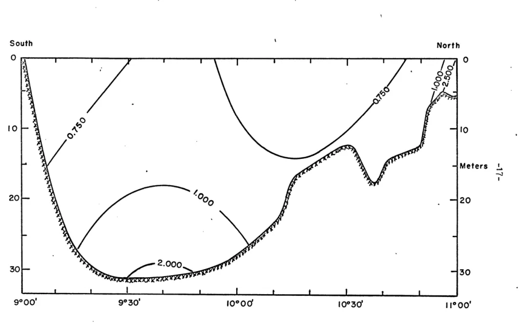
Tablazo Bay, as can be seen from Figures

5-9.

are north-south sections from the Gulf of Venezuela to the southern end of the Lake.

These figures, as well as Figures 10 and 11, indicate that the chlorinity in the Lake has a different pattern and, therefore, the physical processes governing the diffusion of chlorides in the Lake are probably not the same as those in the Straits and Tablazo Bay.

Figures

5-9

in the Straits has been affected by seasonal and long-term

variations in the fresh-water velocity. In March 1954 (Figure

5),

when the fresh-water balance was _{negative, the 2.500 ppt} line of constant chlorinity (isochlor) intersected the bottom of the Straits very near the northern entrance to the Lake. Since the chlorinity at the bottom of the Lake near the center

South _North

0I Mt _{nAj _}

9*00d 9*3 0' 10'000 10* 30' 11000'

FIGURE 5. North-south cross-section from the Gulf of Venezuela to the south end of Lake

Maracaibo showing chlorinity, C(ppt), distribution in March 1954, From Redfield(1955).

Meters _,

South 0 r-. 9*00' 9*30' IOod 10*3' North 0 10 Meters i 20 30 11000'

FIGURE 6. _{North- south cross-section from the Gulf of Venezuela to the south end of Lake}

South 0 rr-10 20 30 North -iO 9*00 FIGURE 7. - 10 Meters - 20 SAA00- 30 I I 9*30' 10000 10030 II00'

North-south cross-section from the Gulf of Venezuela to the south end of Lake Moracaibo showing chlorinity, C(ppt), distribution in March of 1963. From

South 0 20 30 North --- n 0 9000' FIGURE 8. -10 Meters -20 -3 9030' 10000' 10030' 11000'

North-south cross-section from the Gulf of Venezuela to the south end of Lake Maracaibo showing chlorinity, C(ppt) , distribution in December 1963.

North 10 10 - ' 20- 30-9000' FIGURE 9. 9*30' 10*00' 10*30'

North-south cross-section from the Gulf of Venezuela to the south end of Lake Maracaibo showing chlorinity, C(ppt), distribution in June 1966. From

unpublished data of the I.N.C.

- Meters

-20

-30

1000

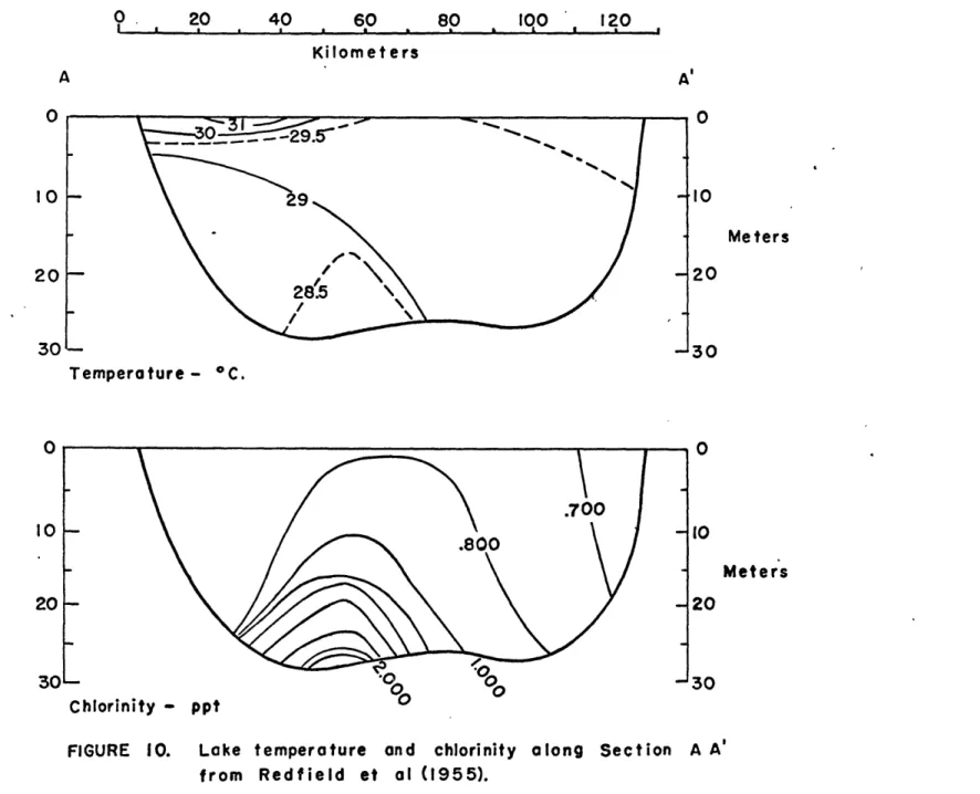
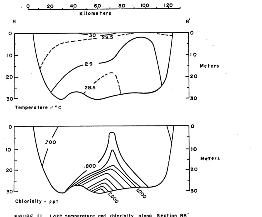
Kilometers A 10

_-o

FIGURE 10. Lake temperature and chlorinity along Section A A'

from Redfield et al (1955). Meters 20 30 Meters 20 30 0 20 40 60 80 t00 e a a1,

20 40 60

Kilometers

Temperature -a'C

FIGURE 1I. Lake temperature and chlorinity from Redfield et al (1955). 0 1O Meters 20 30 N) Meters along Section BB 8,0 a 1QO , Ig0 , 20 30

-23-Lake was receiving water of this chlorinity from the Straits. In May 1954 (Figure 6) the 2.500 ppt isochlor moved north, almost to the Gulf of Venezuela, presumably as a result of

the positive fresh-water balance during this month. A similar

shift in isochlors is seen by comparing March 1963 (Figure 7),

a dry month on the average, although no hydrological data is available for this period, and December 1963 (Figure 8), a wet

month. The data from 1963 also show how the chlorinity increased

both in the Lake and 'the Straits between 1954 and 1963. The

most recent data is from a survey made in June 1966 by the I.N.C. (Figure 9), which give an indication of the present chlorinity distribution in the Straits and the Lake.

1.9 Flushing time of the Lake.-- The average time a molecule

of salt remains in the Lake determines how the Lake water will

react to factors altering the accession of water or salt into

the Lake. This time is given'by the ratio of the Lake volume

to the fresh-water discharge. The volume of Lake Maracaibo is

approximately 25 x 1010 cubic meters. The total annual average

fresh-water discharge, as determined from Figure 2, is about' 50 x 109 cubic meters. Dividing the Lake volume by the

fresh-water discharge gives a value of about

5

flushing, or residence, time for a salt molecule in the Lake.

intrusion problem in the Straits of Haracaibo and Tablazo Bay

were begun by Corona (1966) using the one-dimensional model for

a long narrow channel originated by Ippen and Harleman (1961).

In this method the salinity, S, and the longitudinal

velocity, u, are taken _{as instantaneous, average values over}

each cross-section. For Lake Maracaibo the salinity, S, is

related to the chlorinity, C, by the following formula:

S

=

1.SOS

C

+0.0

0.10.1)

Because the channel is assumed to be long and narrow, variations across the channel are neglected, and therefore,

variables are functions of time, t, and longitudinal distance along the channel, x, only.

The one-dimensional conservation of salt equation for a channel of constant cross-sectional area is given by:

LA CI/=.

c

(1.10.2)

where DI is the apparent diffusion coefficient. This coefficient x

includes the mass transfer by turbulent diffusion and the important nass transfer by internal currents caused by the density difference between salt and fresh water. The fluid velocity, u, is equal to the sum of the tidal velocity, u(x,t), and the fresh-water velocity, U, due to the outflow from the

Lake. Equation (1.10.2) becomes:

~S

(~t~-U~

K#

(1.10.3)

The negative sign in the fresh-water velocity term appears because the origin of x is taken at the ocean entrance and is measured positive in the landward direction.

If the fresh-water discharge is relatively constant during a period of time of the order of several days or a week, a quasi-steady state salinity distribution should result in the estuary. That is, the one-dimensional salinity distribution at

instants of time differing by one tidal cycle should be the

same. This should be expecially true at low water slack (L.W.S.)

since the salinity distribution at high water slack may be more

influenced by daily variations in tidal amplitude.

At the moment of low water slack, the salinity at any station should be close to its minimum value. In addition, at

low water slack both DS and u(x,t) are momentarily zero.

Z>t

Equation (1.10.3) can then be written:

~U

0)SLWVS

C)

DS~

(1-10-4)

vhere SLS = salinity at low water slack and is a function of

x only.

-26-high water slack is given by the low water slack distribution curve displaced longitudinally by a distance equal to the tidal excursion. This is equivalent to stating that within one-half of a tidal period:

L

c

+

=

aA

(1-10-5)

C)t

D X

Equation (1.10.4) can be integrated if the functional

dependence of D1 _x and boundary conditions on the salinity, S, are given.

The functional dependence of DI on x is assumed to be the

x

following form:

D

C

Therefore, at x = 0 (ocean entrance), D' = D', while at

x 0

x = -B (seaward of x = 0), D' -o oo , and for large x (in the

x

positive, or landward, direction), DI-->O.

X

That D. approaches an infinite value at x = -B is consistent with the fact that if the estuary was imagined to extend to

x = -B, an infinite anount of mixing would be required to maintain

a constant salinity at low water slack.

The boundary conditions on the salinity are assumed to be

dS

-27-x = -B, where S is the ocean salinity.

The solution to equation (1.10.4) is then given by:

_U (x,+)

B

3

WS

--

so

If the salinity is knom at low water slack for at least two

points (values of x) the parameters DI and B can be determined

from equation (1.10.7).

For actual field conditions, where the basic assumptions

used to derive the mathematical model are not exactly satisfied, it has been found that two dimensionless salinity parameters:

Dt and 2'B

0

UB _uOT

mhere u0 is the maxmum flood tide velocity at the ocean entrance,

and T is the tidal period, correlate with a dimensionless combination of variables known as the "estuary number". The

estuary number is defined as follows:

P F

-28-where,

= tidal prism, the volume of sea water entering t the estuary on flood tide.

F = Froude number, uo , u being the maximum

flood tide velocity; g, the force per unity mass due to gravity; and h, the mean channel

depth.

Qf = fresh-water discharge T = tidal period

Using salinity measurements obtained from the Straits of Maracaibo and Tablazo Bay during surveys made by the I.N.C.,

Corona (1966) was able to calculate the values of D' and B

from equation (1.10.7) for various values of fresh-water

D

discharge and tidal velocity. The two salinity parameters, D and, 2'i\'B , were calculated and plotted against the estuary

number PT 2 , and the results are shown in Figures 12 and 13.

From these Tigures estimates of DI and B can be obtained for given values of tidal velocity-and fresh-water discharge.

4aximum and minimum intrusion lengths for the Tablazo Bay-Straits of Maracaibo estuary can then be predicted as shown in Table III of Ippen (1966).

It should be kept in mind that the analysis described above can be used with confidence only in the Straits and Tablazo Bay, and does not apply to the diffusion of salt in the Lake proper. It does however furnish information about the salinity at the northern end of the Lake where the Straits join the Lake.

40 -I--i--i-i-li- I I I I 10-27rB 5 uT I I I1 A 11 £I 1 -1s 0.003 0.D 0.1 0.6 * (Estuary Number) OfT

FIGURE 12. Basic salinity distribution parameters in the

Straits of Marocaibo. From Corona (1966).

50 -- r r-rr- I r I--r -r a - tidal amplitude 0 h channel depth 10-D' U B 0. - --a003 0.0 Pt 0.1 0.9 PQF2 (Estuary Number) Q T /

FIGURE 13. Basic salinity distribution parameteirs in the

Straits of Maracaibo. From Corona (1966).

-I----I----I--1 I I I ' '

0 0

-In this sense it gives a boundary condition for the diffusion of

salt into the Lake, and will therefore be important in an

analysis 'of the entire Tablazo Bay-Straits of Maracaibo-Lake

Maracaibo system.

An investigation which has bearing on the salinity problem in the Lake proper is a model study by Stockhausen (1964). In this investigation a scale model of the Lake was constructed and

salt was added to simulate the salinity distribution in the Lake. The model was then placed on a rotating platform and a wind stress

was applied. The resulting salinity distribution measured in the model agreed well with the prototype and indicated in a quali-tative way .that the wind stress and rotation of the Earth play an

important role in the dynamics of the Lake. These processes are

considerably different than those acting in the Straits and Tablazo Bay, and any analysis of salt diffusion in the Lake must

take into account these same processes.

1.11 Scope of the present investigation.-- It has been emphasized in previous sections that the physical processes affecting the diffusion of salt in the Lake are different from those in the Straits and Tablazo Bay. The diffusion of salt in the Straits and Tablazo Bay has been adequately described by Corona (1966) as

indicated in a previous paragraph. To obtain a unified analysis

31

-the salt diffusion in -the Lake. The purpose of this work is to develop a mathematical model of the dynamical processes affecting the Lake circulation. The diffusion of salt will play an

important part in this mathematical model, as will the effects of wind stress and the rotation of the Earth.

The results of the theoretical investigation will be

compared with the field data obtained by Redfield et al (1955). These data will be used because they provide the most complete

information on velocity and salinity profiles in the Lake.

That the dynamical picture has not changed appreciably since

Redfieldts study is suggested by the shapes of the isochlors

in Figures

5-9,

velocity and salinity profiles would be helpful for establishing the validity of the theoretical model.

II. DEVELOPIET OF T HE IMATIEMATICAL MODEL

2.1 Equations of motion.-- The equations required to describe

the diffusion of salinity and momentum in an incompressible

rotating fluid are the momentum equations, continuity equation,

equations of state, and salt diffusion equation. For axially

symmetric flow, the momentum equations in the radial, azimuthal, and vertical directions, respectively, are:

U

₊

.. .

C)r'

.

r

Ciif

+JL L)

)

3

D-uX

C)e

3

tA

5-iL

ns LA

Ir

+

ns

V.

C) -i

I-+

C')

-- - V-

L

qL

L)

-33-The equation of continuity:

(

)

The equation of state:

-= P I . (2.1

.5)

The equation of salt diffusion:

.. -t. LA . C) (2.1.6)

C t m3

Az D.[S + \k D _r S

The dependent variables, r, z, and t are the radial and

vertical coordinates and time, respectively, where r is positive

outwards and z is positive upward and parallel to the gravity force. The independent variables, u, v, w, , and S are the

radial, azimuthal and vertical velocities, pressure, density and salinity, respectively. -\ and are the horizontal

-34-the horizontal and vertical coefficients of eddy diffusivity.

g is the force per unit mass due to gravity. Cx is a coefficient

relating the density to the salinity and f is the Coriolis

paramter, 2.0 sin , where

.0

the Earth and P is the latitude measured northward from the equator. The 12KS system of units will be used throughout, except where noted.

2.2 ant assumptions.-- The following assumptions will be

used in this work:

(1) The motions are small enough so that the inertial terms

will be negligible.

(2) Frictional effects are confined to small

boundary-layers on the top and bottom.

(3) The major portion of the Lake is in geostrophic

equilibrium, that is, the pressure is balanced by

the Coriolis force.

(h)

4),

This implies that dynlamic effects due to the Earth's sphericity can be ignored.

(5)

constant.

(6) The variations in density are small enough to be

negligible, except where they are associated with

the gravity term. This is the Boussinesq approximation.

(7) The density is a linear function of salinity. This

inplies that CK is a constant.

(8) The Lake is initially at rest and stratified in such

a way that the salinity is a linear function of the depth only.

(9) After the Lake has been set into motion the pressure field can be separated into two portions. One portion is a hydrostatic term resulting from the Lake's

initial stratification, and the other a small pertur-bation caused by the motion. Mathematically, this can be stated:

f(r,

:)

=f

0

(Z)

f4-

(,,)

(2.2.1)

The first two being a constant term and a tern which is a linear function of the depth only. This describes the condition of the Lake while it is at rest and is an exact solution to equation (2.1.6). The third

component is a small perturbation resulting from the

motion. Mathematically, this can be stated:

S~

t,

=so+

sS

-)

The first two terms, S. + v , will be referred to in later sections as the long-term

component.

2.3 Scaling the eouations.-- Exact solutions to the system of

equations (2.1.1) - (2.1.6) are difficult to find. It has been

found, however, that for certain scales of motion the complexity

of these equations can be reduced while retaining the important

features of the flow. A technique which has been successful is to first reduce the equations to dimensionless form, identify

important terms in the scaled equations and then use the nethods of singular perturbation theory to find an approximate solution.

-36-Several investigators have used this method in the study of diffusion processes in a rotating fluid. Greenspan and Howard (1.963) investigated the time-dependent motions of a homogeneous fluid in a rotating cylinder vhose vertical and

horizontal dimensions were approximately the same. Barcilon

and Pedlosky (1967a, 1967b) were concerned with the steady

motion of a temerature-stratified fluid in a rotating

cylinder of similar dimensions as Greenspan and Howard.

Holton (1964) developed a model for the time-dependent motion of a thermally stratified fluid in a rotating basin with a large ratio of horizontal-to-vertical dimensions, but he rather

arbitrarily ignored the effects of temperature diffusion. The following investigation will be concerned with the time-dependent motions of a salt-stratified fluid in a rotating basin of large horizontal dimensions and small vertical dimension.

In this respect it is similar to Holton's work, the major

difference being that the diffusion processes whnich Holton neglected will be taken into account.

The appropriate scaling for a stratified fluid in near-geostrophic equilibrium, and subject to viscous forces, is

-37-(f=V~f

gAAY

L

V4P % VfL S'

where the primed variables are dimensionless, L is a characteristic horizontal dimension, H is a characteristic depth, and V is a

characteristic azimuthal velocity. All other variables and constants have been defined previously.

Certain dimensionless numbers will occur in the equations:

(1) Mechanical Rossby Number - - =

4 L

This is a measure of how much the fluid departs from

a state of rigid rotation.

(2) Internal Rossby Number - 6

=

This is a measure of how much the fluid departs from the initial linear vertical stratification.

(3) Ekman Number -

E

This is a measure of the thickiess of the frictional

boundary layers at the top and bottom.

(h) Aspect Ratio - /

(5) Rotational Richardson Number -

=

This is a measure of the initial stratification.

(6)' _{Horizontal Prandtl Number - Cr}

.

(7) Vertical Prandtl Number

-(8)

This is a measure of the anisotropic nature of the turbulence.

The quantities &SH and &Sv occurring in (2) and

(5)

of the Lake to the edge and the variation of salinity from the top to the bottom, respectively.

In the perturbation expansion which follows it will be

assumed that the internal Rossby number, 6, the mechanical

Rossby number,

,

and the rotational Richardson number,

(

of the same order. There is, of course, no a priori justification

for these assumptions. However, in Section III the theory will be compared with actual field data and the values of important constants estimated. The above dimensionless numbers can then be calculated, and it will be showrn that assumptions made as to their magnitude is, in fact, consistent with the observed behaviour of the Lake.

-39-one (1), as suggested by Sverdrup (1942), and the vertical Prandtl number, CUI , according to Hunk and Anderson is about 10. The

physical dimensions of the Lake determine the aspect ratio. Making use of the above, the dimensionless forms of the equations are:

+ Lt"uc'U' _{+ )r' 2_u'} .'L I-Cs=

32U

QM~f

-4

+E

D Y11

FZ

₊

E.c~U3

~t.

Lk'

3 nS5

XL

Iw

xAY'~

E

r )I

_r

(2-3-4)

L

3- -L

-fols

L[es"

E

;A

4

-) t'

-The equation of state, equation (2.15), has been eliminated

by naking use of the Boussinesq approximation.

2.4 Perturbation expansion.-- Folloring the example of Holton (1964) and Barcilon and Pedlosky (1967a, 1967b), the

independent variables, u, vp w, , and S are expanded in terms

of the square root of the Ekman number, 0" = , which is a

measure of the thickness of the frictional boundary layers at the top and botton, and, as mentioned previously, is assumed to

be small:

tA(4

E

E''

Lk IE ( V 8

Lk n 5 ( V: !: ) +

)

l2.

cir(v1'') =

O

E

(nr

-,a't)

E

(2.4-4)

'Ih81r

V

nhk

n

5o

T

(u , --- ) are the values of the variables in the interior of the fluid, and (u' B nB , ----) and

(ut V , are the correct'ions to the interior flow

nB nB

in the bpundary layers at the top and bottom, respectively, and

are functions of r, t, and the stretched coordinates, = ,

=

E

satisfy the boundary conditions at the top and bottom, and must vanish in the interior.

2.5 Interior expansion.-- The interior flow, to zero order, is

obtained by substituting the expanded form of the variables

(equations (2.h.1) - (2.h.5)) into equations (2.3.1) - (2.3.5)

and collecting terms whose coefficients are of the order unity.

The resulting interior equations are:

-(1 ' _ _(2.5.1)

OIL -L (2o.2

-h3-')'

9TO

=0

c3~

I2s

44

!4r

2.6 Boundary layer expansion.-- The zero-order expansion for

the corrections to the interior flow in the top boundary

layer (zt = 1) is found to be:

.4T. t = Q05

)

: _*S

r 8

I

775vo

0

r

)

c)~tLr'

Similarly, in the bottom boundary layer (zi = 0):

LAJL

L

8

--0

,E8

r\

.

D

A

/

2.7 Boundary conditions.-- The boundary condtions to be

satisfied are: at zt = 0 u= 0 v = 0, wt = 0, 0 at z' 1 Ut 0 _{=, (rt),}

*

=

where /C (rt) is the dimensionless wind stress.

at rI = I u' = 0, V' = 0, - 0 a) r0 at rt = 0 U1 , vt, I t, 31 are finite (2.6.9) (2.6.10) + '3X

J ro P

.46-at t' = 0

u' = vt = W1 = St = 0

2.8 Solutions.-- The boundary layer equations (2.6.1) - (2.6.10)

are the same as those first solved by Elonan (1905) with the exception of equations (2.6.5) and 2.6.10) involving the

diffusion of salt, which were not used by Elnan because he was

concerned with a homogeneous fluid. Since no solutions to

equations (2.6.5) and (2.6.10) can be found which allow So

and S' to vanisa in the interior, except St S oB 0

oB oB o13

the solutions to equations (2.6.1) - (2.6.10) for the boundary

conditions given in paragraph 2.7 must be the same as those given by Ekman. These solutions are:

-47-TlQ S

e

(2.8.4)

The boundary conditions for the vertical velocity are obtained by integrating the continuity equations (2.5.4),

(2.6.4) and (2.6.9): at z' = 0 (2.8.5) I at z, = 1

05-1

--

4..

JA

K>

(iX

'r

=

-of V, O,-'

7YL-

-148-The results of the integration are:

at zt = 0 -_ at zI = 1

,AAr

V.dyL~~J

Ox

_r

_aI'L

_J

For the interior it is evident from equations (2.5.1) and

(2.5.3) that the pressure, p0 , can be treated as a stream-function, VI, which satisfies the equation:

(2.8.7)

(2.8.9) + #

+2t.

0all

L7-

with boundary conditions:

at z, = 0 2. ~~i2~ ~jat( (2.8.10)

DYL

7 Lv

oI)

5~LA

)r,

E

)KA"~~TY

dV.\c)21

Dih.(

'I,

DI )

CrIr

12

q)-)

..-_.oarl

I

7J,

at rt = 0

'Va'

C)r

'T =

0

To complete the solution-it is necessary to specify the

wind stress,

i

useful form of the wind stress is:

(2.8.15)

where u-₁ (t') is the unit stop-function, J (kr") is the Bessel function of first kind and order one, and k is chosen such that Jj(k) = 0.

Making use of Laplace transforms, the partial differential equation (2.8.9) reduces to:

(2.8.16)

1

C-)

s

--f

+

ah1.

-os

while the boundary condition at zt = 0, equation (2.8.10),

becomes:

1/.

L

. 1'K

-t~K1~

O:.

P

1

7--

_I

₄

?tc'f

OT.

+]

and:

ci

₎

e

et

e

dt

(2

I4

-

(I,

Inverting equations (2.8.16) and (2.8.17) leads to the solution: (t)

(z~

IL)

-

]LA

(t- )

tLA t)

From this the azimuthal velocity and the salinity perturbation in the interior can be determined. The baroclinic and barotropic modes of the azimuthal velocity are, respectively:

1 (1)(2.8.23)

CLSQ._3x

(2.8.24)

The baroclinic mode, equation (2.8.23), responds to that part of the pressure field for which the pressure is not a function of the density only, whereas the barotropic mode,

equation (2.8.24), responds to that part of the pressure field for which the pressure is a function of density only. In a

barotropic fluid the lines of constant pressure and constant

density are everywhere parallel, which is not the case for a baroclinic fluid. In general, the pressure field of a fluid

barotropic component and the resulting velocity field uill have

a barotropic and baroclinic component as was found above. For

a fluid which is in quasi-geostrophic equilibrium, as Lake

Maracaibo has been assumed to be, the barotropic velocity

component will be independent of the depth, whereas the

baroclinic mode irill have a dependence upon the depth. This

is evident from equations (2.8.23) and (2.8.2).

The salinity perturbation is given by:

The zero order velocity and perturbation salinity fields

for the entire fluid are:

e

-Ar

LA

Q )

4e

4r(

(2.8.2>

T

k#

W4

-i

T

LA

4T

-o U V: )

=

eI

E

-

-56-III. APPLICATION OF THE THSORY TO LAKE M1YAACAIBO

3.1 Estimating the size of important constants.-- The mathematical model derived in Section II characterizes the time-dependent flow of a rotating, stratified, and incompressible fluid for a rather specific set of conditions. These conditions are: (1) viscous effects are confined to thin layers at the top and bottom of the fluid; (2) the initial stratification of the fluid is small;

(3) the fluid motion differs only slightly from a state of solid rotation; (h) the stratification due to the fluid motion differs only by a small amount from the initial stratification; and

(5)

necessary to compare the theory with actual field data from the Lake. The most exhaustive field study of Lake aracaibo was made by Redfield et al (1955) in the Spring of 1954. Figures

10 and 11 show Lake chlorinity and Figure 15 shows the azimuthal velocity profiles obtained during this survey. This data will be used to determinc the validity of the theory for tho

steady-state case only, since no suitable time series is available for the investigation of tine-dependent motions.

The theory can be compared ith the data only if the numerical values of the constants, OC , f, g, H, L, V, ASv,

& SH' 4 ' )., W., and, , are known. These constants

have determined in the following manner:

C - the coefficient relating the density to the salinity

is given by Lafond (1951) as 1 .53 x 1

o-3

f - the Coriolis parameter, 2 C. sin 4 , is calculated for a latitude of 90 501, which corresponds, approximately, to the center of the Lake. -- , the angular velocity

of the Earth, is 0.73 x 10

-4

f = 2 x 0.73 x 1oh~ x sin(90 501) = 2.48 x 10-5 sec.-1 g - the force per unit mass due to gravity is 9.81 meters2

sec.~1

H - the characteristic depth of the Lake is approximately

30 meters. Actual depth and idealized depth are

compared in Figure

14.

L - the characteristic radius of the Lake is approximately

60 x 1o3 meters as shown in Figure 14.

&S V- the variation in salinity from top to bottom is

obtained from the data of Redfield et al (1955). From

Figures 10 and 11 the chlorinity, C, at the top in the middle of the Lake is about 0.80 ppt, and at the bottom about 0.20 ppt. Converting chlorinity to

salinity by means of equation (1.10.1):

Sv = 1.805 x C(top) - 1.805 x C(bottom)

0 20 I 1 I 40 I I 60 I I 80 I I 100 I I 120 I I A Kilometers I I - II -- I -- ---Meters 0 10 Meters 20 30

FIGURE 14. Comparison of idealized Lake (dashed lines) with

actual Lkd (solid lines) along Sections AA' and BB.'

20

30 10

SH- the variation in salinity from the middle of the Lake to the edge of the Lake is also obtained from Redfield. Figures 10 and 11 show that the chlorinity at the top varies from 0.80 ppt at the center to 0.70 ppt at the

- edge, and, at the bottom, from 2.00 ppt at the center

to 1.00 ppt at the edge. Again making use of

equation (1.10.1):

AS

ASH(bottom) = (1.00 - 2.00) x 1.805 =

-1.81

The average of these two values:

ASH(top) + ASH(bottom) = -0.99 ppt

2 will be used.

- the vertical eddy viscosity is determined by the size

of the frictional boundary layers. For a rotating fluid the thickness of these boundaries is given by the so-called Ekman depth, .

In Lake Maracaibo this depth is approximately

4

15(c).

Elman depth = 4.0 =:

and

V - the characteristic velocity, and

- the horizontal eddy diffusivity, are calculated in the

-60-From Figure 15(c) the azimuthal velocity at the surface, approximately midway between the center and edge of the Lake, is 0.55 meters per second. The dimensionless form of the theoretical steady-state (t = 00)

azimuthal velocity at the surface (z' 1, = 0, = 10)

and midway between the center and edge (r' =

),

equation (2.8.26), is:

Recalling that:

Y

0 0.2 0.4 (a) FIGURE 15. 0. 0.2 0.4 (b) Azimuthal Velocity,

Velocity profiles at various po sitions in measured by Redfleld et al (1955).

the motion is counterclockwise.

0 0.2 (c) meters/second Meters 20 . 0.4 0.6 the Lake as The sense of

-62-then:

A'

Applying the numerical values of C(

L SV calculated previously:

, g, f, , and

E' aX

513.(0

io

The dimensional azimuthal velocity is related to the dimensionless velocity, as follows:

r\'

₌

_V

The dimensional azimuthal velocity at the surface, midway

between the center and edge of the Lake is then:

L 2 0,. 0

cr

TT~~

2L(z x 155 x to _c(,131

A v. 2.&VS %

i o*"S

'2.A

't

Vo-

-63-The constant, k, is the first root of the equation J (k) = 0. From Jahnke and Emde (1945), k = 3.83,

,and J1 (3.83) = 0.58.

2

IMatching the observed Lake velocity of 0.55 meters

per second with the theoretical velocity:

0.55

2-This equation contains two unknoims, *Ay and V. Therefore, a second equation is needed. The second

equation is provided by the salinity perturbation term.

From equation (2.3.29) the dimensionless form of the

salinity perturbation is:

8.O

x

To

Y

Recalling the scaling procedure of paragraph 2.3,

the dimensional form of the salinity perturbation is

VF

L

_S,

<I

H

-

V

.XO

85-I

The horizontal variation of the theoretical perturbation, 6 (S Szi), from the center of

to the adge is given by:

salinity

the Lake

3

S-q4.~*x

o

V

where the values of JO(3.83) and Jo(o.00) have been determined from Jahnke and Erde (1945).

Equating the theoretical salinity variation to the

actual average variation in the Lake,

ASH

as calculated previously:

0.9 4X3 .. 0

IP\V

V

_2.Lc0

\

Solving the two simultaneous equations:

o.90

= V

Vas

4Kj

3\

0

F

0 -10-L

2,%8 11

-i

T

X

o-3

determines the values of %yand V:

V = 0.03 meters per second

,r= 3.17 x 102 meters2 seconds-1

In paragraph 2.3 it was pointed out that the horizontal

Prandtl number, -, = -Q.

/v,

/96,

10, for most cases of geophysical interest. Applying

these ratios:

y = 3.17 x 102 meters2 seconds-1 = 1.98 x 10~ reters2 seconds 1

The values of these constants as they have been computed

above are given in Table 1. They can also be used to calculate

ihe magnitude of the important dimensionless parameters:

Rotational Richardson H4umber,

30.0

(

-66--Mechanical Rossby Nlunber,_C

cE-v

-0L

=

0.L8I

O.514

x

1c,

Internal Rossby Numbe,±-r

ET %

1

-

53x.

(-

0.C

(

2.&A8?%1\5~

fx(JOo

=0.20O

(30.l

2.48

O-5

%o-2-Symbol Parameter Name Value Units

O< Coefficient relating salinity and density 1.53 x 10-3 ppt-1

f Coriolis paramter 2.48 x 10-5 seconds-1

g Force per unit mass due to gravity 9.81 meters-seconds-2

H Characteristic depth 30.0 meters

L Characteristic radius 60.0 x 103 meters

ASH Magnitude of top-to-bottom salinity -0.99 ppt

variation

as Magnitude of middle-to-edge salinity -2.16 ppt

variation

Horizontal eddy viscosity 3.17 x 102 meters2-secondsl

Vertical eddy viscosity 1.98 x 10~4 meters2seconds1

Y Horizontal eddy diffusivity 3.17 x 102 meters2seconds1

Vertical eddy diffusivity 1.98 x 10- meters 2-seconds1

V Characteristic azimuthal velocity 0.08 meters-seconds~1