Dynamics of bead formation, filament thinning
and breakup in weakly viscoelastic jets
The MIT Faculty has made this article openly available.
Please share
how this access benefits you. Your story matters.
Citation
ARDEKANI, A. M., V. SHARMA, and G. H. McKINLEY. Dynamics
of Bead Formation, Filament Thinning and Breakup in Weakly
Viscoelastic Jets. Journal of Fluid Mechanics 665 (December 6,
2010): 46-56.
As Published
http://dx.doi.org/10.1017/s0022112010004738
Publisher
Cambridge University Press
Version
Author's final manuscript
Citable link
http://hdl.handle.net/1721.1/78938
Terms of Use
Creative Commons Attribution-Noncommercial-Share Alike 3.0
Under consideration for publication in J. Fluid Mech. 1
Dynamics of Bead Formation,
Filament Thinning, and Breakup in
Weakly Viscoelastic Jets
A. M. A R D E K A N I, V. S H A R M A, G. H. M C K I N L E Y
Department of Mechanical Engineering Massachusetts Institute of Technology
Cambridge, MA 02139, USA (Received 28 July 2010)
The spatiotemporal evolution of a viscoelastic jet depends on the relative magnitude of capillary, viscous, inertial and elastic stresses. The interplay of capillary and elastic stresses leads to formation of very thin and stable filaments between drops, or to ‘beads-on-a-string’ structure. We show that by understanding the physical processes that control different stages of the jet evolution it is possible to extract transient extensional viscosity information even for very low viscosity and weakly-elastic liquids which is a particular challenge using traditional rheometers. The parameter-space at which a forced jet can be used as an extensional rheometer is numerically investigated using a one-dimensional nonlinear free surface theory for Oldroyd-B and Giesekus fluids. The results show that even when the ratio of viscous to inertio-capillary time scales (or Ohnesorge number) is as low as 𝑂ℎ ∼ 0.02, the temporal evolution of the jet can be used to obtain elongational properties of the liquid.
1. Introduction
Understanding the instability and breakup of polymeric jets is important for a wide variety of applications including spraying of fertilizers and paints and ink jet printing applications (Hoath et al. (2009); Morrison & Harlen (2010)). Such fluids are typically only weakly viscoelastic and the jetting/breakup process involves a delicate interplay of capillary, viscous, inertial and elastic stresses.
In this study, we investigate the growth and evolution of surface-tension-driven insta-bilities on an axisymmetric viscoelastic jet using nonlinear theory for a range of different constitutive equations. The initial growth of the disturbances can be predicted using linear instability analysis for small perturbations. A viscoelastic jet is initially more un-stable when compared to a Newtonian fluid of the same viscosity and inertia (Middleman (1965), Goldin et al. (1969), and Brenn et al. (2000)). As the local radius of constrictions in the jet decreases under the action of surface tension, elastic stresses grow and become comparable to the capillary pressure, leading to formation of a uniform thread connect-ing two primary drops. This ‘beads-on-a-strconnect-ing’ structure can be captured by quasi-linear constitutive models like the Oldroyd-B model, and the radius of the thin cylindrical lig-ament connecting the beads necks down exponentially in time (Bousfield et al. (1986); Entov & Yarin (1984)). The finite time breakup of the jet observed experimentally can be captured using the nonlinear Giesekus model or FENE model (Fontelos & Li (2004)). The temporal evolution of a viscoelastic fluid thread depends on the relative magnitude of the viscous, inertial, and elastic stresses and the capillary pressure (Bhat et al. (2010)).
In order to study this inertio-elasto-capillary balance in detail for a jet, two dimensionless
parameters are defined: the Ohnesorge number 𝑂ℎ = √𝜂0
𝜌𝛾𝑅0 which is the inverse of
the Reynolds number based on a characteristic capillary velocity 𝛾
𝜂0 and, secondly, the
intrinsic Deborah number 𝐷𝑒 = 𝜆√𝛾/𝜌𝑅3
0 defined as the ratio of the time scale for
elastic stress relaxation, 𝜆, to the “Rayleigh time scale” for inertio-capillary breakup of
an inviscid jet, 𝑡𝑅=√𝜌𝑅3
0/𝛾. In these expressions, 𝜌 is the fluid density, 𝜂0 is the fluid
zero shear viscosity, 𝛾 is the surface tension, 𝑅0 is the initial radius of the jet, and 𝜆 is
the relaxation time associated with the polymer solution.
Sch¨ummer & Tebel (1983) proposed that an extensional rheometer based on jetting can be used to obtain comparative information about elongational behavior of polymer solutions. Here, we show that by understanding the physical processes that control each stage of the spatiotemporal evolution in the jet profile it is possible to extract tran-sient extensional viscosity information even for very low viscosity and weakly-elastic liquids, at high strain rates relevant to spraying and jetting. The jet extensional rheome-ter is especially useful since filament-stretching rheomerheome-ters can typically only be used to measure the extensional viscosity of moderately viscous non-Newtonian fluids, at least in 1g. Gravitational sagging is a limiting factor in filament-stretching devices for low-viscosity polymeric liquids (Anna et al. (2001)). Similarly the capillary breakup elonga-tional rheometry (CABER) technique faces challenges for low-viscosity elastic polymer solutions. The limitations arise from the finite time it takes for the device to impose the initial axial deformation to the sample. In addition, the Ohnesorge number needs to be large enough (𝑂ℎ ≳ 0.14) to be able to distinguish the effect of viscosity on the local necking and breakup of the filament (Rodd et al. (2005)). For aqueous solutions with surface tension coefficient of 𝛾 ≃ 0.07𝑁/𝑚 and plate radius of 3𝑚𝑚, the lower bound on
the measurable viscosity is 𝜂0≳ 63 𝑚𝑃 𝑎𝑠.
Achieving a quantitative understanding of Sch¨ummer & Tebel (1983)’s experimental measurements was limited by the large experimental parameter space involved. We use our numerical simulations to explore the range of operating conditions over which a jet can effectively be used to measure the transient extensional viscosity of the liquid. We show that this is limited by three independent factors: 1) calculation of the tensile stress difference in the thread connecting the drops must be directly connected to the evolution in the local jet radius; i.e. an “elasto-capillary balance” must be established; 2) the range of diameters over which this elasto-capillary regime is established must be experimentally-resolvable; 3) the formation of secondary droplets along the thread must be suppressed. In the present work, we show how the perturbation frequency of forcing that is imposed on the jet can be used to control those conditions and determine the optimal range of excitations for using the self-thinning dynamics of fluid jet breakup as a means of performing transient extensional rheometry. We call this rheometer, Rayleigh-Ohnesorge Jet Extensional Rheometer (ROJER).
2. Problem Description
In this study, we consider an axisymmetric slender jet of polymeric liquid using the Giesekus and Oldroyd-B constitutive equations (Bird et al. (1987)). The radius of the jet
𝑅(𝑧, 𝑡) slowly varies along the liquid jet and we only consider the leading-order
Dynamics of bead formation, filament thinning & breakup in weakly viscoelastic jets 3
momentum along the jet can be written as follows:
∂𝑅2 ∂𝑡 + ∂ ∂𝑧(𝑣𝑅2) = 0 (2.1) 𝜌 ( ∂𝑣 ∂𝑡 + 𝑣 ∂𝑣 ∂𝑧 ) = −𝛾∂𝜅∂𝑧 + 3𝜂𝑠𝑅12∂𝑧∂ ( 𝑅2∂𝑣 ∂𝑧 ) +𝑅12∂𝑧∂ (𝑅2(𝜎𝑧𝑧− 𝜎𝑟𝑟)) (2.2) 𝜅 = 1 𝑅(1 + 𝑅2 𝑧)1/2 − 𝑅𝑧𝑧 (1 + 𝑅2 𝑧)3/2 (2.3)
where 𝑣(𝑧, 𝑡) is the axial velocity; 𝜂𝑠 and 𝜂𝑝are the solvent and polymer contribution to
the total viscosity, respectively (total viscosity 𝜂0 = 𝜂𝑠+ 𝜂𝑝); 𝑅𝑧 indicates the partial
derivative ∂𝑅
∂𝑧; 𝜎𝑧𝑧 and 𝜎𝑟𝑟 are the diagonal terms of the extra-stress tensor and they can
be calculated as follows: 𝜎𝑧𝑧+ 𝜆 ( ∂𝜎𝑧𝑧 ∂𝑡 + 𝑣 ∂𝜎𝑧𝑧 ∂𝑧 − 2 ∂𝑣 ∂𝑧𝜎𝑧𝑧 ) +𝛼𝜆𝜂 𝑝𝜎 2 𝑧𝑧= 2𝜂𝑝∂𝑣∂𝑧 𝜎𝑟𝑟+ 𝜆 ( ∂𝜎𝑟𝑟 ∂𝑡 + 𝑣 ∂𝜎𝑟𝑟 ∂𝑧 + ∂𝑣 ∂𝑧𝜎𝑟𝑟 ) +𝛼𝜆 𝜂𝑝𝜎 2 𝑟𝑟 = −𝜂𝑝∂𝑣∂𝑧 (2.4)
where 𝜆 is the relaxation time of the liquid; 𝛼 is a positive dimensionless parameter corresponding to the anisotropy of the hydrodynamic drag on the polymer molecules and is called the mobility factor (Giesekus (1982)). For 𝛼 = 0, the Oldroyd-B model is recovered. Equation (2.2) can be written in conservative form as (Fontelos & Li (2004); Li & Fontelos (2003)): 𝜌 ( ∂(𝑅2𝑣) ∂𝑡 + ∂(𝑅2𝑣2) ∂𝑧 ) = ∂𝑧∂ [ 𝑅2(𝛾𝐾 + 3𝜂 𝑠∂𝑣∂𝑧+ 𝜎𝑧𝑧− 𝜎𝑟𝑟 )] = 𝜋1∂𝐹∂𝑧 (2.5) 𝐾 = 1 𝑅(1 + 𝑅2 𝑧)1/2 + 𝑅𝑧𝑧 (1 + 𝑅2 𝑧)3/2 (2.6) where ∂𝜅
∂𝑧 = −𝑅12∂𝑧∂ (𝑅2𝐾) (Entov & Yarin (1984)) and 𝐹 is the total tensile force exerted
over the cross sectional area of the jet. Forest & Wang (1990) asymptotically derived slender jet model for a viscoelastic fluid and Bousfield et al. (1986) numerically solved a 1D model using a Lagrangian formulation. The model used in this manuscript is similar to that of Bousfield et al. (1986) but an Eulerian formulation is used. The above equations are solved using an implicit finite difference scheme on a staggered grid and computations of very low Oh number and De number jets can be achieved. 1400 grid points are used
and the time step is set equal to 3 × 10⁻⁵𝑡𝑅. Periodic boundary conditions are used and
the the initial shape of the jet, at 𝑡 = 0, is described as 𝑅 = 𝑅0(1 + 0.01 cos(𝑘𝑧)) where
𝑘 is the wavenumber. The evolution and breakup of a viscoelastic jet can be represented
in terms of five dimensionless parameter: 𝑂ℎ, 𝐷𝑒, the dimensionless wavenumber 𝑘𝑅0,
the solvent viscosity ratio 𝛽 = 𝜂𝑠
𝜂0, and the mobility factor 𝛼.
The results from the simulation can be used to calculate extensional viscosity of the viscoelastic liquid. For a slender liquid jet, the local strain rate can be calculated as:
˙𝜀 = ∂𝑣∂𝑧 = −𝑅2 𝑑𝑅𝑑𝑡 (2.7)
The transient uniaxial extensional viscosity, can be written as:
𝜂+
𝐸 ≡𝜏𝑧𝑧− 𝜏˙𝜀 𝑟𝑟 = 3𝜂𝑠+𝜎𝑧𝑧− 𝜎˙𝜀 𝑟𝑟 (2.8)
As defined, the extensional viscosity is a locally varying quantity and to realize a useful rheometer, we need to generate a spatially and temporally constant extension rate. In
0 0.2 0.4 0.6 0.8 1 0 0.05 0.1 0.15 0.2 0.25 0.3 0.35
dimensionless growth rate
k
Inviscid Oh=0 Viscous Oh=0.04 De=0 Viscoelastic Oh=0.04 De=0.8 Viscoelastic Oh=0.04 De=10
a b c R -2 0 2 0 5 10 15 20 25 30 z t=4 2 . 8 a R -2 0 2 0 5 t=2 4 . 8 5 z b R -2 0 2 0 5 t=2 5 . 2 z c 0 0.2 0.4 0.6 0.8 1 0 0.05 0.1 0.15 0.2 0.25 0.3 0.35
dimensionless growth rate
k
Inviscid Oh=0 Viscous Oh=0.4 De=0 Viscoelastic Oh=0.4 De=1 Viscoelastic Oh=0.4 De=10
a b c R -2 0 2 0 5 t=5 6 z c R -2 0 2 0 5 10 t=5 2 z b R -2 0 2 0 5 10 15 20 25 30 z t=4 2 . 8 a
Figure 1: Dispersion curve predicted by linear instability of a viscoelastic jet and com-parison to a purely viscous jet and an inviscid jet. The formation of satellite droplets is suppressed at wavenumbers larger than 𝑘 ≳ 0.85 at 𝑂ℎ = 0.04 and 𝑘 ≳ 0.75 at 𝑂ℎ = 0.4. Jet profiles are calculated using non-linear analysis.
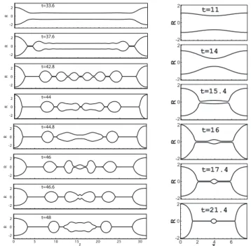
z R 0 5 10 15 20 25 30 -2 0 2 z R 0 5 10 15 20 25 30 -2 0 2 z R 0 5 10 15 20 25 30 -2 0 2 z R 0 5 10 15 20 25 30 -2 0 2 z R 0 5 10 15 20 25 30 -2 0 2 z R 0 5 10 15 20 25 30 -2 0 2 z R 0 5 10 15 20 25 30 -2 0 2 z R 0 5 10 15 20 25 30 -2 0 2 t=33.6 t=37.6 t=42.8 t=44 t=44.8 t=46 t=46.6 t=48 t=11 t=16 t=17.4 t=21.4 t=15.4 t=14
Figure 2: Temporal evolution of an Oldroyd-B liquid jet at 𝑂ℎ = 0.04, 𝐷𝑒 = 0.8, 𝛽 = 0.27,
𝛼 = 0: a)𝑘 = 0.2; b)𝑘 = 0.8.
the elasto-capillary regime, we obtain a thin uniform tread with a radius which decreases exponentially in time resulting in a constant strain rate(Clasen et al. (2006)).
𝑅𝑚𝑖𝑑(𝑡) 𝑅0 ≈ ( 𝜂𝑝𝑅0 2𝜆𝛾 )1/3 exp(−𝑡/3𝜆); ˙𝜀𝑚𝑖𝑑= 3𝜆2 (2.9)
Dynamics of bead formation, filament thinning & breakup in weakly viscoelastic jets 5 R -2 0 2 0 5 10 15 20 25 30 z t=42.8
Figure 3: Space-time diagrams for thinning and breakup of an Oldroyd-B liquid jet at different disturbance wavenumbers, 𝑂ℎ = 0.04, 𝐷𝑒 = 0.8, 𝛽 = 0.27 , 𝛼 = 0. For each axial
position and time, the contour plots of 𝑙𝑜𝑔10[𝑅(𝑧, 𝑡)] are shown. Simulations are continued
till a minimum dimensionless radius of 10−3.5= 0.0003 is obtained. Dimensionless axial
position, 𝑧, varies between 0 and 2𝜋/𝑘. a)𝑘 = 0.2 b)𝑘 = 0.675 c)𝑘 = 0.8 d)𝑘 = 0.9
3. Results and Discussion
In this section, we show how the temporal evolution of a jet can be used to extract the extensional properties of a low viscosity weakly-elastic liquid. In particular, we discuss computational rheometry for an aqueous polymeric solution with zero shear viscosity
𝜂0 = 3.7𝑚𝑃 𝑎𝑠, 𝜂𝑠= 1𝑚𝑃 𝑎𝑠, relaxation time 𝜆 = 0.17𝑚𝑠, density 𝜌 = 1000𝑘𝑔/𝑚3, and
surface tension 𝛾 = 0.06𝑁/𝑚 moving out of a nozzle with the radius of 𝑅0 = 140𝜇𝑚.
Fluids with similar rheological properties are discussed by Hoath et al. (2009). The dimensionless parameters for such a liquid are 𝑂ℎ ∼ 0.04, 𝛽 = 0.27, 𝐷𝑒 = 0.8. As described in the introduction, filament stretching or CABER devices cannot be used to measure the tensile property of such a low-viscosity liquid because of the rapid timescale for breakup and formation of satellite beads. The formation of satellite droplet must be inhibited for the purpose of extensional rheometry and we next show that this can be
achieved by varying the perturbation wavenumber, 𝑘𝑅0, in the liquid jet.
In order to consider effects of the imposed perturbation wavenumber on the jet mor-phology, let us first examine the prediction of the linear instability theory for a viscoelastic liquid jet. The dispersion relation between the wave growth rate and the wavenumber for a temporal instability of a viscoelastic jet in an inviscid gaseous environment was first given by Middleman (1965) [see also Goldin et al. (1969) and Brenn et al. (2000)] and is plotted in figure 1 (a). It should be noted that all the quantities presented in this section are dimensionless; time is nondimensionalized using the Rayleigh time, 𝑡𝑅; length using
𝑅0, and stress using 𝛾/𝑅0. For reference we also show the dispersion curve for a more
viscous liquid at 𝑂ℎ ∼ 0.4 and 𝛽 = 0.5 in figure 1 (b). The corresponding limits for a viscous Newtonian jet (𝐷𝑒 = 0) and an inviscid jet (𝑂ℎ = 0) are plotted for both cases. A viscoelastic liquid has a larger growth rate compared to a Newtonian liquid of the same viscosity. The fluid elasticity enhances the growth of instabilities whereas viscous effects result in a more stable jet. The effect of varying the excitation wavenumber also has a pronounced effect on the nonlinear evolution of the jet at long time. Snapshots of the nonlinear jet profiles developed by different wavenumbers reveals three distinct regimes. Increasing the dimensionless wavenumber, from 𝑘 = 0.2 to 𝑘 = 0.9 (denoted by a, b, c respectively), results in the formation of multiple, single, and zero secondary droplets as the jet evolves. For a wavenumber smaller than the one corresponding to the maximum growth rate, 𝑘 = 0.2, traveling capillary waves are observed, the details of
which are shown in figure 2. Multiple satellite droplets form and they migrate towards the center, they coalesce with another droplet to form a larger intermediary drop. Li & Fontelos (2003) investigated the effects of elastic forces on the drop dynamics including drop migration, oscillation, merging and drop drainage for highly elastic liquids. Bhat
et al. (2010) showed that inertia is required for the initial formation of such structures
and that satellite beads do not form if the liquid is sufficiently viscous. Here we show that increasing the critical wave number suppresses the formation of satellite beads for low viscosity and weakly-elastic liquids. It is clear that the spatiotemporal dynamics of the thinning jet greatly impact the ability to use the process of jet breakup as a rheometer. The information shown in the frames of figure 2 can be condensed into the space-time
diagram plotted in figure 3 (a). Contour plots of 𝑙𝑜𝑔10(𝑅) in the 𝑧 − 𝑡 plane show the
oscillations of both the satellite and main droplets due to capillary forces. A thin axially uniform thread forms between these droplets and an exponential thinning can be clearly observed in the thread connecting the main drop and the satellite drops (green-blue regions). For the wavenumber corresponding to the maximum growth rate, 𝑘 = 0.675, a single satellite droplet forms (figure 3 (b)). Both the satellite and primary droplets oscillate due to interaction of capillary and inertia. The period of oscillation for second harmonic infinitesimal-amplitude perturbations of a drop of an inviscid liquid is given
by Rayleigh (1879) as 𝑇 = √𝜋
2𝑅 3/2
𝑑𝑟𝑜𝑝, equal to 𝑇 = 5.8 and 𝑇 = 0.96 for the main and
satellite droplets, respectively. The period of oscillation of the main drop and secondary drop for 𝑘 = 0.675 determined from figure 3 (b) are 5.4 and 1.06, respectively. Lamb (1932) considered the effect of small viscosity on the small-amplitude oscillation of drops
and showed that the damping ratio for second harmonic oscillation is 𝜉 = 2.5𝑂ℎ√
2 𝑅𝑑𝑟𝑜𝑝.
Basaran (1992) calculated the nonlinear oscillation of a viscous drop and showed that the period of oscillation increases as disturbance amplitude rises. The above calculations are for Newtonian fluids; Bauer & Eidel (1987) and Khismatullin & Nadim (2001) considered the effect of fluid viscoelasticity on the small amplitude vibration of drops.
As the disturbance wavenumber increases beyond the one corresponding to the maxi-mum growth rate, 𝑘 = 0.8, the size of the secondary droplet decreases and the oscillations of the satellite droplet are dampened more rapidly (figure 3 (c)). For a wavenumber of
𝑘 = 0.9 close to the cutoff wavenumber, we see the formation of an axially-uniform thread
which is more appropriate for extensional rheometry (figure 3 (d)).
We next investigate how the temporal evolution of a jet can be used to measure the tensile rheological properties of a viscoelastic liquid. For a viscoelastic liquid at 𝑂ℎ = 0.4,
𝐷𝑒 = 1, 𝛽 = 0.5, 𝑘 = 0.9 the jet radius thins in the center and main drops form as
shown in figure 1 (b). The corresponding axial velocity field and radius of the jet are plotted in figure 4 (a). The velocity profile shows regions of homogeneous elongational flow in the cylindrical ligament and the magnitude of the extension rate is equal to
˙𝜖 = 2
3𝐷𝑒 (Entov & Hinch (1997)). At later times, as the perturbation amplitude grows
nonlinearly, the elastic stress grows in the jet and the elasto-capillary regime given by equation (2.9) can be clearly observed. The radius of the uniform thread in the center thins exponentially in time and a beads-on-a-string morphology forms (Clasen et al.
(2006)). In this regime (𝑡 ⩾ 45) the tensile stress difference, 𝜏𝑧𝑧− 𝜏𝑟𝑟, at the midpoint of
the filament is approximately equal to the capillary stress (1/𝑅𝑚𝑖𝑑) as shown in figure 4 (b). The extensional viscosity of the liquid can be calculated using equations (2.7) and (2.8) and is plotted in figure 4 (b). Initially the polymeric stress is small and the Trouton ratio, defined as𝜂+𝐸
𝜂0, is equal to 3𝛽. Then a viscous dominated plateau with Trouton ratio
𝜂+
𝐸/𝜂0= 3 is observed as expected for a linear viscoelastic fluid with constant viscosity.
Dynamics of bead formation, filament thinning & breakup in weakly viscoelastic jets 7 z 0 1 2 3 4 5 6 7 -6 -4 -2 0 R v dε/dt 1 2/3De t 0 10 20 30 40 50 10-4 10-3 10-2 10-1 100 101 102 103 (dε/dt)mid 1/Rmid (τzz-τrr)mid (ηE/η0)mid
Figure 4: Midpoint properties of an Oldroyd-B liquid jet at 𝑂ℎ = 0.4, 𝐷𝑒 = 1, 𝛽 = 0.5,
𝑘 = 0.9, 𝛼 = 0, 𝑡 = 52. a) Jet radius, axial velocity, and extension rate are plotted.
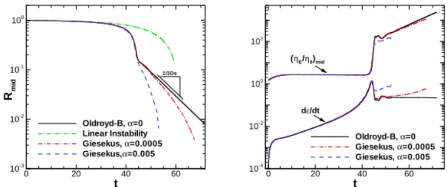
b)Capillary stress is a good representative of the normal stress difference in the elasto-capillary regime. t Rm id 0 20 40 60 10-3 10-2 10-1 100 Oldroyd-B,α=0 Linear Instability Giesekus,α=0.0005 Giesekus,α=0.005 1/3De t 0 20 40 60 10-4 10-2 100 102 Oldroyd-B,α=0 Giesekus,α=0.0005 Giesekus,α=0.005 dε/dt (ηE/η0)mid
Figure 5: Comparison of Oldroyd-B and Giesekus jets at 𝑂ℎ = 0.4, 𝐷𝑒 = 3, 𝛽 = 0.5,
𝑘 = 0.9. a)Radius of the jet b)extension rate and extensional viscosity at the midpoint.
to the stretch of polymer molecules. In an experiment, the local extension rate in the thinning ligament can be calculated by measuring the radius of the midpoint. Due to symmetry, the spatial derivative of stress is zero at the midpoint and equation (2.4) can be integrated to calculate the tensile stress difference. For an Oldroyd-B fluid we have
(𝜏𝑧𝑧− 𝜏𝑟𝑟)𝑚𝑖𝑑= 3𝛽𝑂ℎ ˙𝜀 + 𝑒2𝜀−𝑡/𝐷𝑒 ∫ 𝑡 0 2(1 − 𝛽) 𝑂ℎ 𝐷𝑒˙𝜀(𝑡′)𝑒−2𝜀(𝑡 ′)+𝑡′/𝐷𝑒 𝑑𝑡′ + 𝑒−𝜀−𝑡/𝐷𝑒∫ 𝑡 0 (1 − 𝛽) 𝑂ℎ 𝐷𝑒˙𝜀(𝑡′)𝑒𝜀(𝑡 ′)+𝑡′/𝐷𝑒 𝑑𝑡′. (3.1)
This implies that the transient extensional viscosity of the viscoelastic liquid can be calculated using an experimentally obtained extension rate together with equation (3.1). In a Giesekus fluid, the variation in the level of strain-hardening influences the necking process (see figure 5). As the mobility factor increases, the breakup occurs earlier. Unlike Oldroyd-B fluid, where constant strain rate occurs in the elastocapillary regime, strain rate does not remain constant for larger Giesekus parameters.
In order to show how measurements of extensional viscosity will be affected as the perturbation frequency varies at low Ohnesorge number, in figure 6 we compare the
t 0 5 10 15 20 25 10-8 10-6 10-4 10-2 100 102 (τzz-τrr)mid, k=0.9 1/Rmid, k=0.9 (τzz-τrr)mid, k=0.675 1/Rmid, k=0.675
(a) Stress at the midpoint
t 0 10 20 30 10-6 10-4 10-2 100 102 104 Rz=6.2 1/Rz=6.2 (τzz-τrr)z=6.2 1/3De (b) Stress at 𝑧 = 6.2, 𝑘 = 0.675
Figure 6: Estimates of the elastic stress of a low viscosity and weakly-elastic jet modeled by the Oldroyd-B fluid at different disturbance wavenumbers, 𝑂ℎ = 0.04, 𝐷𝑒 = 0.8,
𝛽 = 0.27, 𝛼 = 0. k kmax D e 0 0.3 0.6 0.9 10-1 100 101 102
With satellite droplet No satellite droplet d a c b k kmax O h 0.4 0.6 0.8 1 10-2 10-1
100 With satellite droplet
No satellite droplet kmax
Figure 7: Effects of the wavenumber, Deborah, and Ohnesorge numbers on the jet mor-phology for an Oldroyd-B liquid jet at 𝛽 = 0.6 and 𝛼 = 0. Wavenumbers smaller than
𝑘 ≲ 𝑘𝑚𝑎𝑥 are not useful for the purpose of extensional rheometry due to the formation
of satellite droplets and the resulting oscillation. a)𝑂ℎ = 0.02 The space-time diagrams associated with cases a, b, c, and d are plotted in figure 8. b)𝐷𝑒 = 1. The broken blue line shows the locus of the most unstable mode from linear theory 𝑘𝑚𝑎𝑥(𝑂ℎ, 𝐷𝑒). stress difference at the midpoint for two different wavenumbers at 𝑂ℎ = 0.04. It can be seen in figure 6 (a) that for a wavenumber close to the cutoff wavenumber, the stress at the midpoint can be approximated by the capillary stress, or in dimensionless form
(𝜏𝑧𝑧− 𝜏𝑟𝑟)𝑚𝑖𝑑 ≈ 𝑅𝑚𝑖𝑑1 . Whereas for a smaller wavenumber, 𝑘 = 0.675, a satellite bead
is observed at the midpoint and the stress oscillates due to oscillation of the drop. In this case the capillary stress is not a good estimation of the normal stress difference. However, in this case we can measure the stress in the thread connecting the satellite and the main droplet where the thread once again thins exponentially as exp(−𝑡/3𝐷𝑒). Figure 6 (b) shows the radius, capillary stress, and normal stress difference of the thin thread at 𝑧 = 6.2. Here, the capillary stress is a better approximation of the normal stress difference in the thread, as compared to the jet midpoint which corresponds to the satellite droplet. The stress at 𝑧 = 6.2 varies quasi-periodically with frequencies driven
Dynamics of bead formation, filament thinning & breakup in weakly viscoelastic jets 9 R 0 0 2 4 6 t =46.8 z R 0 0 5 t =72 z R -2 0 2 0 5 10 t =72 z R -5 0 5 0 10 20 30t =210 z
Figure 8: Space-time diagrams for an Oldroyd-B liquid jet at different disturbance wavenumbers and Deborah number, 𝑂ℎ = 0.02, 𝛽 = 0.6 , 𝛼 = 0. For each axial
po-sition and time, contour plots of 𝑙𝑜𝑔10(𝑅) are shown corresponding to the state diagram
of figure 7. a)𝑘 = 0.9, 𝐷𝑒 = 1.67 b)𝑘 = 0.8, 𝐷𝑒 = 3 c)𝑘 = 0.55, 𝐷𝑒 = 25 d)𝑘 = 0.2,
𝐷𝑒 = 300
by both the main and satellite drops. If there is no satellite droplet then the radius
of the large end drops can be calculated to be 𝑅3
𝑑𝑟𝑜𝑝 = 3𝜋/2𝑘. These inertio-capillary
oscillations are increasingly damped as viscous effects increase. For an Ohnesorge number
𝑂ℎ ⩾ 0.4√(2)/𝑅𝑑𝑟𝑜𝑝 = 0.34𝑘1/3, the drop response is over damped and no oscillation
occurs. For 𝑘 = 0.9, the Ohnesorge number should be larger than 𝑂ℎ ≳ 0.4. As shown in figure 4, the main drop motion is over damped for 𝑂ℎ = 0.4, and no oscillation is observed.
Lastly, we explore the operational parameter-space for a jet elongational rheometer by considering the combined effects of the excitation frequency, Deborah, and Ohnesorge numbers. Two slices of the three-dimensional parameter-space (𝑘, 𝐷𝑒, 𝑂ℎ) are shown in figure 7. For shorter wavenumbers, higher viscosity (𝑂ℎ) and higher elasticity (𝐷𝑒) are required to inhibit the formation of a satellite droplet. The effect of increasing elasticity (𝐷𝑒) is illustrated by the space-time diagrams for cases a-d in 8. Cases a and b are most appropriate for extensional rheometry since no satellite droplet occurs in the elasto-capillary regime. However, case b is distinct in the sense that initially a satellite droplet appears to develop near the midplane but the liquid in the secondary droplet subsequently drains into the main droplets. As shown in figures 7 and 8, wavenumbers smaller than
𝑘 ≲ 𝑘𝑚𝑎𝑥 are not useful for the purpose of extensional rheometry due to the formation
of single (case c) or multiple satellite droplets (case d) and their subsequent oscillation and interaction.
4. Conclusions
We have shown that a perturbed jet undergoing capillary thinning can be used suc-cessfully as an elongational rheometer for measuring tensile properties of even weakly viscoelastic polymer solutions. The formation of satellite droplets can be suppressed
the thread to thin as a single axially-uniform filament. For a weakly viscoelastic liquid
(𝐷𝑒 = 𝜆/𝑡𝑅= 𝜆
√
𝛾/𝜌𝑅3
0 = 0.8), a jet extensional rheometer will be effective for
Ohne-sorge numbers as low as 𝑂ℎ ≃ 0.02. For 𝑂ℎ < 0.02, additional calculations show that the formation of satellite droplets is unavoidable even at wavenumbers close to unity.
REFERENCES
Anna, S.L., McKinley, G.H., Nguyen, D.A., Sridhar, T., Muller, S.J., Huang, J. & James, D.F. 2001 An interlaboratory comparison of measurements from filament-stretching rheometers using common test fluids. J. Rheol. 45, 83–114.
Basaran, O.A. 1992 Nonlinear oscillation of viscous liquid drops. J. Fluid Mech. 241, 169–198. Bauer, H.F. & Eidel, W. 1987 Vibration of a visco-elastic spherical immiscible liquid system.
Z. Angew. Math. Mech. 67, 525–535.
Bhat, P.P., Appathurai, S., Harris1, M.T., Pasquali, M., McKinley, G.H. & Basaran, O.A. 2010 Formation of beads-on-a-string structures during breakup of viscoelastic fila-ments. Nature Physics .
Bird, R., Armstrong, R. & Hassager 1987 Dynamics of polymeric Liquids. John Wiley. Bousfield, D.W., Keunings, R., Marrucci, G. & Denn, M.M. 1986 Nonlinear-analysis of
the surface-tension driven breakup of viscoelastic filaments. J. Non-Newtonian Fluid Mech.
21 (1), 79–97.
Brenn, G., Liu, Z. & Durst, F. 2000 Linear analysis of the temporal instability of axisym-metrical non-Newtonian liquid jets. Int. J. Multiphase Flow 26, 1621–1644.
Clasen, C., Eggers, J., Fontelos, M.A., Li, J. & McKinley, G.H. 2006 The beads-on-string structure of viscoelastic threads. J. Fluid Mech. 556, 283–308.
Eggers, J. 1997 Nonlinear dynamics and breakup of free-surface flows. Rev. Mod. Phys. 69, 865–929.
Entov, V.M. & Hinch, E.J. 1997 Effect of a spectrum of relaxation times on the capillary thinning of a filament of elastic liquid. J. Non-Newtonian Fluid Mech. 72 (1), 31–53. Entov, V.M. & Yarin, A.L. 1984 Influence of elastic stresses on the capillary breakup of dilute
polymer solutions. Fluid Dyn. 19, 21–29.
Fontelos, M.A. & Li, J. 2004 On the evolution and rupture of filaments in Giesekus and FENE models. J. Non-Newtonian Fluid Mech. 118 (1), 1–16.
Forest, M.G. & Wang, Q. 1990 Change-of-type behavior in viscoelastic slender jet models.
J. Theor. Comput. Fluid Dyn. 2, 1–25.
Giesekus, H. 1982 A simple constitutive equation for polymer fluids based on the concept of deformation-dependent tensorial mobility. J. Non-Newtonian Fluid Mech. 11 (1-2), 69–109. Goldin, M., Yerushalmi, J., Pfeffer, R. & Shinnar, R. 1969 Breakup of a laminar capillary
jet of a viscoelastic fluid. J. Fluid Mech. 38, 689–711.
Hoath, S.D., Hutchings, I.M., Martin, G.D., Tuladhar, T.R., Mackley, M.R. & Vadillo, D. 2009 Links between ink rheology, drop-on-demand jet formation, and print-ability. J. Imaging Sci. Techn. 53, 041208.
Khismatullin, D.B. & Nadim, A. 2001 Shape oscillations of a viscoelastic drop. Physical
Review E 63 (6, Part 1), art. no.–061508.
Lamb, H. 1932 Hydrodynamics. Dover, New York.
Li, J. & Fontelos, M.A. 2003 Drop dynamics on the beads-on-string structure for viscoelastic jets: A numerical study. Phys. Fluids 15 (4), 922–937.
Middleman, S. 1965 Stability of a viscoelastic jet. Chem. Eng. Sci. 20, 1037–1040.
Morrison, N.F. & Harlen, O.G. 2010 Viscoelasticity in inkjet printing. Rheol Acta 49, 619– 632.
Rayleigh, Lord 1879 On the capillary phenomena of jets. Proc. R. Soc. Lond. 29, 71–97. Rodd, L.E., Scott, T.P., Cooper-White, J. & McKinley, G.H. 2005 Capillary break-up
rheometry of low-viscosity elastic fluids. Appl. Rheol. 15, 12–27.
Sch¨ummer, P. & Tebel, K.H. 1983 A new elongational rheometer for polymer solutions. J.