A numerical model of the ionospheric signatures of time-varying magneticreconnection: I. ionospheric convection

HAL Id: hal-00317209

https://hal.archives-ouvertes.fr/hal-00317209

Submitted on 1 Jan 2004

HAL is a multi-disciplinary open access

archive for the deposit and dissemination of

sci-entific research documents, whether they are

pub-lished or not. The documents may come from

teaching and research institutions in France or

abroad, or from public or private research centers.

L’archive ouverte pluridisciplinaire HAL, est

destinée au dépôt et à la diffusion de documents

scientifiques de niveau recherche, publiés ou non,

émanant des établissements d’enseignement et de

recherche français ou étrangers, des laboratoires

publics ou privés.

time-varying magneticreconnection: I. ionospheric

convection

M. Lockwood, S. K. Morley

To cite this version:

M. Lockwood, S. K. Morley. A numerical model of the ionospheric signatures of time-varying

magneti-creconnection: I. ionospheric convection. Annales Geophysicae, European Geosciences Union, 2004,

22 (1), pp.73-91. �hal-00317209�

Annales

Geophysicae

A numerical model of the ionospheric signatures of time-varying

magnetic reconnection: I. ionospheric convection

M. Lockwood1,2and S. K. Morley2

1_{Rutherford Appleton Laboratory, Chilton, Oxfordshire, UK}

2_{Department of Physics and Astronomy, University of Southampton, Southampton, Hampshire, UK}

Received: 9 September 2002 – Revised: 19 May 2003 – Accepted: 2 June 2003 – Published: 1 January 2004

Abstract. This paper presents a numerical model for

pre-dicting the evolution of the pattern of ionospheric convection in response to general time-dependent magnetic reconnec-tion at the dayside magnetopause and in the cross-tail cur-rent sheet of the geomagnetic tail. The model quantifies the concepts of ionospheric flow excitation by Cowley and Lockwood (1992), assuming a uniform spatial distribution of ionospheric conductivity. The model is demonstrated us-ing an example in which travellus-ing reconnection pulses com-mence near noon and then move across the dayside mag-netopause towards both dawn and dusk. Two such pulses, 8 min apart, are used and each causes the reconnection to be active for 1 min at every MLT that they pass over. This ex-ample demonstrates how the convection response to a given change in the interplanetary magnetic field (via the reconnec-tion rate) depends on the previous reconnecreconnec-tion history. The causes of this effect are explained. The inherent assumptions and the potential applications of the model are discussed.

Key words. Ionosphere (ionosphere-magnetosphere

in-teractions; plasma convection) – Magnetospheric physics

(magnetosphere-ionosphere interactions; solar

wind-magnetosphere interactions)

1 Introduction

Cowley and Lockwood (1992) developed a conceptual model of how ionospheric flow is excited on timescales shorter than the substorm cycle. Prior to this work, conceptual and empir-ical models of convection had been inherently steady-state in nature, in that they predicted a given pattern of ionospheric convection for a given prevailing orientation of the inter-planetary magnetic field (IMF) (e.g. Cowley, 1984; Heelis et al., 1982; Heppner and Maynard, 1987; Holt et al., 1987; Hairston and Heelis, 1990; Reiff and Burch, 1985; Weimer, 1995). Such models did not consider the previous history

Correspondence to: M. Lockwood (m.lockwood@rl.ac.uk)

of the IMF nor the phase of the substorm cycle. The same was true of the models of the corresponding patterns of ionospheric (Friis-Christensen et al., 1985) and field-aligned (Iijima et al., 1978; Erlandson et al., 1988) currents.

1.1 Steady-state and time-varying convection

Some fundamental principles of time-varying and steady-state electrodynamic ionosphere-magnetosphere coupling are illustrated in Fig. 1, from Lockwood and Cowley (1990). Figure 1a shows how a magnetopause reconnection X-line

AB maps down geomagnetic field lines to its ionospheric

projection, a dayside merging gap ab. Similarly, an X-line

DE in the cross-tail current sheet maps to its projection de

in the nightside ionosphere, and the “Stern gap” CF maps to the polar cap diameter, cf . Consider the Faraday loop, fixed in space, ABba: Faraday’s induction law, relating the electric field E and the change in the magnetic field B is, in integral form: I ABba E · dl = 8AB−8ab=∂/∂t Z ABba B · da, (1)

where dl is an element of length around the loop ABba and

dais an element of a surface area bounded by that loop. The

left-hand side (LHS) of Eq. (1) is equal to the difference in

voltages (8AB−8ab) because two segments of the loop, Aa

and Bb, are field-aligned and, on large spatial scales at least, ideal-MHD applies and field-parallel electric fields are zero (i.e. E · dl = 0 for Aa and Bb). In steady-state, all time

derivatives are zero and thus 8AB = 8ab. In non-steady

situations these voltages differ by the induction term on the right-hand side (RHS) of Eq. (1).

Similarly, application of the same logic to the loop CFf c

shows that the transpolar voltage 8cf equals the Stern gap

voltage 8CF in steady state and application to the loop

DEed shows that the nightside merging gap voltage 8de

1 A B F C D E a b f e a b c d e f Φ Φ Φ Φde Φ Φ Φ Φab Φ ΦΦ Φcf Y X Z Φ Φ Φ ΦCF Φ Φ Φ ΦAB Φ Φ Φ ΦDE a). b).

Fig. 1. Schematic of voltages in the magnetosphere generated by the solar wind flow and by magnetic reconnection. (a) A view of the magnetosphere from interplanetary space at northern mid-latitudes in the mid-afternoon sector, with the GSM axes marked. The dashed line is the equatorial magnetopause and the thick lines AB and DE are active reconnection sites in, respectively, the magnetopause and cross-tail current sheet. CF is the Stern gap in interplanetary space. Aa, Bb, Cc, Dd, Ee, and Ff are all magnetic field lines. (b) A view looking down on an ionospheric polar cap with 12:00 MLT to the top and 06:00 MLT to the right. The thin lines bd and ae are “adiaroic” (non-reconnecting) segments of the open-closed field line boundary (OCB), while ab and de are the dayside and nightside merging gaps, the projections of the reconnection X-lines AB and DE. The reconnection X-line voltages 8ABand 8DEare not, in general, equal to the corresponding merging gap voltages in the ionosphere,8aband 8de, because of induction effects. The polar cap voltage 8cf applies across the polar cap diameter cf which maps to the Stern gap, CF , across which the voltage is 8_CF.

steady conditions. Applying Faraday’s law to the ionospheric polar cap boundary yields:

I abde E · dl = 8ab−8de= ∂/∂t Z abde Bi·da = Bi∂Apc/∂t. (2)

In this case, the non-reconnecting or “adiaroic” (meaning “not flowing across” – see Siscoe and Huang, 1985) seg-ments of the open-closed boundary, bd and ea, have zero boundary tangential electric field because they do not map to active reconnection X-lines zero (i.e. E · dl = 0 for

bd and ea) and thus the LHS of Eq. (2) equals the

volt-age difference (8ab−8de). Given that 8ab is the rate of

flux transfer into the polar cap and 8de is its rate of

trans-fer out of the polar cap, Eq. (2) is effectively the continuity

equation for the total open flux. The ionospheric field Bi

is constant to within a few percent (this is often referred to as the “ionospheric incompressibility” condition) and this al-lows derivation of the RHS of Eq. (2) which shows that de-partures from steady-state are manifested in changes of the

polar cap area, Apc. In steady state, the RHS of Eq. (2) is

zero and 8ab = 8de. Application of the same logic to the

two halves of the polar cap bound by Faraday loops abcf and

fcde yields that 8ab = 8de = 8cf and thus, from above,

8ab =8de =8cf =8AB =8DE =8CF under

steady-state conditions. In this case, the electric field in interplane-tary space maps spatially down the open field lines to give the polar cap electric field (Banks et al., 1984; Clauer and Banks, 1988) and all the voltages shown in Fig. 1 are the same.

However, Eqs. (1) and (2) show that induction terms, rep-resented by the time derivatives, mean that these simplifica-tions do not apply in time-dependent cases. For timescales too short for these steady-state concepts to apply, Cowley and Lockwood (1992) replaced the steady-state paradigm of the interplanetary electric field mapping spatially to the iono-sphere with the concept of perturbation from zero-flow equi-libria caused by time-dependent production (8AB>8DE) or

loss (8AB<8DE) of the total open polar cap flux, {BiApc}.

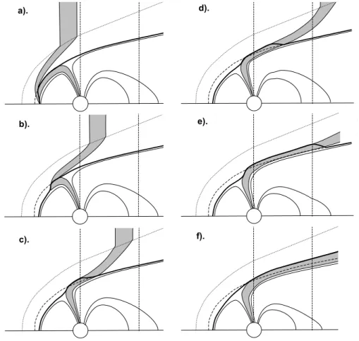
The solar wind flow causes newly-opened flux, produced by magnetic reconnection in the dayside magnetopause, to be appended to the tail lobe. The process is illustrated schemat-ically in Fig. 2 by a series of noon-midnight cross-sections of the northern hemisphere of the magnetosphere. The area shaded grey in each part denotes newly-opened flux

pro-1 a). b). c). d). e). f).

Fig. 2. Schematic noon-midnight cross-sections of the northern hemisphere magnetosphere, illustrating the evolution of newly-opened flux, shaded gray, as it is appended to the tail lobe by the solar wind flow following subsolar reconnection. The heavy solid line is the magnetopause current sheet, the dashed line shows its location prior to the reconnection pulse which produced the newly-opened flux. The dotted line is the bow shock and the two vertical lines are magnetospheric cross-sections at [X]GSM=0 and [X]GSM= −30 RE. Thin lines are geomagnetic field lines.

duced by a pulse in the reconnection rate, in this case at an X-line at the nose of the magnetosphere. The vertical

dashed lines show the [Y Z]GSMplanes of the Geocentric

So-lar Magnetospheric coordinate system at [X]GSM = 0 and

[X]GSM = −30 RE. In Fig. 2a, the reconnection pulse has

just ended and the consequent erosion of the magnetosphere at the nose can be seen by comparing the current magne-topause location (heavy solid line) with its original, pre-pulse position (dashed line). In Fig. 2b the antisunward evolution of the newly-opened flux, under the joint influence of the magnetic curvature force and the magnetosheath flow, can be seen, but the tail lobe at [X]GSM =0 is not yet influenced. In

Fig. 2c the newly-opened flux has been appended to the tail

lobe such that the magnetopause at [X]GSM =0 has flared

outward; however, the tail at [X]GSM = −30RE is yet to

be affected. This does not happen until the time shown in Fig. 2e. Figure 2f shows the situation when the near-Earth magnetosphere has reached a new equilibrium with the new total open flux, with an eroded dayside and a flared tail (com-pare the final and initial magnetopause locations shown by the heavy solid and dashed lines).

The closed field lines in the near-Earth tail, shown in

Fig. 2, are influenced as the newly-opened field lines are ap-pended to the tail. In the far tail, where the tail radius has reached its asymptotic limit, the undisturbed solar wind flow is parallel to the tail magnetopause and the solar wind dy-namic pressure is not a factor. Thus the magnetic pressure in the tail lobe balances the static pressure in the solar wind (the sum of the thermal and magnetic pressures) and increas-ing the tail lobe flux increases the tail’s cross-sectional area (i.e. the tail flares) but the magnetic pressure and field in the far-tail lobes remain constant. However, in the dayside and near-Earth tail, the solar wind dynamic pressure limits the magnetopause expansion and adding newly-opened flux in-creases the pressure in the near-Earth tail. In Figs. 2a–c, the tail pressure has yet to increase as the newly-opened flux has yet to reach that far antisunward. However in Figs. 2d–f, the increase in pressure is causing closed field lines in the tail to be compressed towards the cross-tail current sheet. This compression spreads down the tail as the newly-opened flux evolves antisunward.

Figure 3 presents a qualitative description of the convec-tion patterns that result from the evoluconvec-tion of the newly-opened flux shown in Fig. 2. (It is the purpose of this

pa-1

Fig. 3. Schematic illustration of the Cowley-Lockwood flow excitation model for the example of a single short-lived pulse of subsolar magnetopause reconnection which is completed by time t = 0. The top row is for t = 0, the second row for t = 4 min, the third row for t = 14 min and the fourth row for t>60 min. The first column gives views of the ionospheric polar cap from above. The merging gap ab is marked in (a). The second and third columns show cross-sections of the magnetosphere at [X]GSM = 0 and [X]GSM = −30 RE, respectively, the solid line being the tail magnetopause. The fourth column gives views of the closed field line region in the equatorial plane of the magnetosphere with the [X]GSM axis up the page. The regions shaded grey are closed field lines, bounded by a solid line which is the open-closed boundary; lines with arrows are flow streamlines and the thick black arrows show boundary motions. In row 1, the dot-dash lines give the final zero-flow equilibrium positions that the boundaries will eventually adopt (at t greater than about 60 min). The double dot-dash lines in the top row show the boundary location before the reconnection pulse occurred. In rows 2 and 3, the dashed lines show the equilibrium boundary positions for that instant of time. In row 4, the dotted lines show the boundary locations prior to the first reconnection pulse.

per to make the corresponding quantitative predictions). This schematic is a more detailed adaptation of that given by Cow-ley and Lockwood (1992). The four rows describe the situ-ations at four different times relative to a single, short-lived pulse of magnetopause reconnection. The top row (Figs. 3a– d) corresponds to Fig. 2a and is for time t = 0, just after the

reconnection pulse has taken place but before the ionospheric flow response has commenced. The second row (3e–h) is for t≈4 min and corresponds to Fig. 2c. Field lines evolve

at speed VF over the magnetopause under the influence of

magnetic tension and sheath flow. On the dayside, a constant

field lines will have moved 19 RE by t = 4 min, sufficient to

carry them to near X = 0. The third row (Figs. 3i–l) is for

t ≈14 min. and corresponds to Fig. 2e. Gas dynamic

mod-elling predicts that the sheath flow over the magnetopause

Vshwill average about 0.8 Vswfor X between 0 and −30 RE,

where Vsw is the speed of the undisturbed solar wind

(Spreiter et al., 1966). Along the tail magnetopause we

expect VF≈Vsh≈0.8 Vsw. From this we expect the

newly-opened field lines to move tailward by about 30 REbetween

t = 4 and t = 14 min. The fourth row (Figs. 3m–p) is for

tgreater than about 1 h when the effects of the reconnection

pulse on convection have decayed away completely and cor-respond to Fig. 2f. The four columns in Fig. 3 show different parts of the coupled magnetosphere-ionosphere system and the lines with arrows are flow streamlines. The first column (parts a, e, i and m) gives views of the northern hemisphere polar cap, with noon (12:00 MLT) to the top, 06:00 MLT to the right and 18:00 MLT to the left. The area shaded grey is the closed field line region, delineated by a solid line which is therefore the open-closed field line boundary (OCB). The second column (b, f, j and n) shows cross

sec-tions of the magnetosphere (parallel to the [Y Z]GSM plane)

at [X]GSM =0; the solid line is the magnetopause and the

grey areas show closed field lines threading this tail cross section. The third column (c, g, k and o) is the same as

col-umn 2 for [X]GSM = −30 RE. Column 4 (d, h, l and p) gives

views of the closed field line region in the equatorial plane of

the magnetosphere with [X]GSM up the page and [Y ]GSM to

the left. The horizontal dashed lines in column 4 show the locations of the cross sections given in columns 2 and 3 (and also as shown in Fig. 2).

Row one of Fig. 3 shows the locations of the magne-topause and the open-closed field line boundary immediately after a short-lived reconnection pulse has taken place, imme-diately after the Alfv´en wave has arrived in the ionosphere but before any significant flow has begun (corresponding to Fig. 2a). The open flux in the tail lobe at this time is all “old”, in that it was produced by prior periods of magnetopause re-connection which were sufficiently long before that the resid-ual convection they cause in the near-Earth magnetosphere and ionosphere is negligible. The dashed-double-dot lines give the location of the dayside open-closed boundary just before the reconnection pulse and the dot-dash lines show the final zero-flow equilibrium locations of the open-closed and magnetopause boundaries. These zero-flow equilibrium boundary locations were the key concept introduced by Cow-ley and Lockwood (1992) and provide a way to understand observed flow responses to reconnection changes. We define an equilibrium boundary to be the location such that were a magnetospheric boundary (the open-closed field line bound-ary or the magnetopause) to be at such a location at all MLT, the flow in the magnetosphere-ionosphere system would fall to zero. The production of new open flux perturbs the bound-aries from these equilibrium locations and flow results as the magnetosphere returns towards equilibrium. Note that be-cause newly-opened flux is dragged antisunward by the solar wind, these equilibrium boundary locations will evolve with

time to their final locations shown in rows 1 and 4. Thus we need to make a distinction between the final resting place of the equilibrium boundaries (the dot-dash lines in row 1 of Fig. 3) and their locations at an intermediate instant of time (dashed lines in rows 2 and 3). In row 1, we see that the re-connection pulse has produced two effects; namely, equator-ward motion of the dayside open-closed boundary and Earth-ward erosion of the dayside magnetopause. In Fig. 3a, a re-gion of newly-opened flux has been appended around noon to the ionospheric polar cap (here taken to mean the region of open geomagnetic flux) and this erosion has taken place at the merging gap (ab in Fig. 1 and Fig. 3a). In Fig. 2a we see that the open flux has already moved away from the equato-rial reconnection X-line and so the dayside equatoequato-rial mag-netopause has been eroded inward in Fig. 3d; this erosion takes place at the reconnection site (AB in Fig. 1). How-ever, the newly-open flux has not yet migrated tailward as far

as [X]GSM = −30 RE nor even to [X]GSM = 0 and thus

no effect of the reconnection pulse is yet apparent in either Fig. 3c nor 3b. The final equilibrium locations of the magne-topause, shown as dot-dash lines in row 1, reflect the fact that the reconnection pulse has eroded the total flux in the dayside magnetosphere and the opened flux produced has flared the tail as it is dragged antisunward by the solar wind flow.

In row 2 of Fig. 3, for t = 4 min (corresponding to Fig. 2c),

the open flux produced by the pulse has reached [X]GSM =0

and is perturbing the magnetospheric equilibrium there. In particular, the newly-opened flux is appended to the sun-ward end of the tail lobe. In this case, the dashed lines show the locations of the equilibrium boundary at this time. Note

that the magnetopause at [X]GSM = −30 RE has yet to be

perturbed because the newly-opened flux has not propagated sufficiently far down the tail. In Fig. 3f, we see the flows that

result at [X]GSM =0 because the magnetosphere is

return-ing toward the equilibrium configuration for the new amount of open flux that is present in the near-Earth magnetosphere; this flow is in the tail lobes and corresponds to the antisun-ward flow that has appeared in the polar cap ionosphere as part of the small convection vortices shown in Fig. 3e. This antisunward flow is taking place in the ionosphere after the reconnection pulse has ceased because the OCB between a and b is equatorward of its equilibrium location and is re-laxing poleward. Flow in the ionosphere is incompressible,

in the sense that the ionospheric field strength Bi remains

approximately constant, thus there are no sources and sinks and flow streamlines are closed loops. This means that the antisunward flow in the polar cap must be accompanied by return sunward flow in the auroral oval, completing the vor-tices. The antisunward flow on open field lines couples to the sunward flow on closed field lines through equatorward motion of the adiaroic polar cap boundary toward its new equilibrium position since no flux can cross that boundary. This sunward flow on closed field lines mirrors that seen in the equatorial magnetosphere in Fig. 3h as the eroded day-side magnetopause relaxes back sunward and closed mag-netic flux in the tail is squeezed sunward by the arrival of the new open flux in the tail lobes.

The situation at t = 14 min is similar to that at t = 4 min,

except that the newly-opened flux has reached [X]GSM =

−30 RE and is perturbing the magnetosphere there as well

as at [X]GSM = 0 (as in Fig. 2e). In the ionosphere, this

tailward expansion of the magnetospheric perturbation flow is mirrored in an expansion of the flow pattern away from noon. In column 1 of Fig. 3, r and s are the points sun-ward of which the ionospheric equilibrium boundary loca-tion is perturbed (on the dusk and dawn flanks, respectively). These migrate toward midnight as the newly-opened flux is appended to the tail at increasingly negative [X]GSM.

The last row in Fig. 3 is the idealised situation where the magnetosphere has fully come into equilibrium with the new amount of open flux (corresponding to Fig. 2f). This may take more than an hour and so is unlikely to be re-alised in practice as another source of perturbation (either a second pulse of magnetopause reconnection or the onset of tail reconnection) is very likely to take place before this is achieved. Nevertheless, this idealised state is important as it describes what the magnetosphere-ionosphere system is tending toward at earlier times. In row 4 of Fig. 3, the solid lines are the OCB and magnetopause and the dotted line shows the initial OCB and magnetopause locations, just before the reconnection pulse (as also shown in row 1).

Note that at all times demonstrated in Fig. 3, the recon-nection has ceased; all flow that is present is associated with adiaroic (non-reconnecting) boundaries moving toward their new equilibrium locations with less closed flux on the day-side and more open flux in the tail.

Figure 3 is concerned with a short pulse of magnetopause reconnection. Similar considerations can be applied to a burst of tail reconnection on a range of timescales. How-ever, in this paper we restrict our attention to variations in the magnetopause reconnection rate. Generalisation for steady or variable tail reconnection can be added using similar prin-ciples, as discussed by Cowley and Lockwood (1992) and Lu et al. (2002), but will add to the complexity.

1.2 Observations of ionospheric convection responses to

reconnection rate variations

A rise in the rate of open flux generation (the magnetopause reconnection voltage) is communicated from the magne-topause to the ionosphere by Alfv´en waves which propagate along dayside field lines in 1–2 min. Such rapid responses were first detected by Nishida (1968a, b) who compared data from near-Earth IMF monitors with observations by day-side ground-based magnetometers. The key prediction of the Cowley-Lockwood flow-excitation model is that the majority of the ionospheric flow response to the reconnection pulse at a magnetopause X-line AB is a localised pair of convection vortices, centred on the ends of the merging gap, a and b, and that these vortices expand in MLT away from the

merg-ing gap as the magnetospheric tail at greater [X]GSM is

per-turbed by the newly-opened flux produced by the pulse (as illustrated in Fig. 3).

This expansion has been reported in various

experimen-tal studies. The antisunward propagation of a change in

the ionospheric convection electric field was first reported by Lockwood et al. (1986), who used the EISCAT (Euro-pean Incoherent Scatter) radar to observe the consequent in-crease in F-region ion temperatures following a southward-turning of the IMF, as seen just outside the bow shock by the AMPTE (Active Magnetospheric Particle Tracer Explorer) spacecraft. This heating is caused by collisions between the convecting ions and neutral thermospheric atoms whose mo-tion cannot respond as rapidly. The convecmo-tion increase was shown to have propagated eastward over the two beams of the EISCAT radar in the afternoon sector auroral oval (i.e. away from noon), a cross-correlation analysis showing that the rise was seen first in the beam closer to noon. The lag between the changes seen in the two beams gave a

propa-gation speed of 2.6 km s−1_{in the eastward direction around}

the afternoon sector, i.e. away from noon. The same tech-nique was used to make direct observations of similar propa-gation of convection enhancements associated with transient cusp/cleft auroral events thought to be caused by short-lived (minute-scale) pulses of magnetopause reconnection (Lock-wood et al., 1993a).

This propagation has also been found in surveys of the re-sponse time of the convection change as a function of po-sition. The response time was found to increase with dis-tance from a location near noon, using EISCAT radar ob-servations of the flow in combination with AMPTE obser-vations of the IMF close to the subsolar point of the bow shock. Etemadi et al. (1988) employed a statistical corre-lation analysis, while Todd et al. (1988) made a survey of event studies. A similar result was found by Saunders et

al. (1992) by comparing oscillations in the Bzcomponent of

the IMF to those seen at different stations of the CANOPUS (Canadian Auroral Network for the Open Program Unified Study) magnetometer network and, more recently, by Cow-ley et al. (1998), Khan and CowCow-ley (1999) and McWilliams et al. (2001). These authors have used a variety of radar tech-niques to observe the expanding flow response: Etemadi et al. used vector flows generated by the EISCAT incoherent scatter radar using the beam-swinging technique (which has assumptions and limitations, cf. Freeman et al., 1991); Todd et al. used measurements of line-of-sight flow component and Cowley et al. and Khan and Cowley employed tristatic EISCAT flow observations. McWilliams et al. used data from the SuperDARN (Super-Dual Auroral Radar Network) HF coherent scatter radars with two different techniques: bistatic measurements were possible in localised regions and a more global view was obtained using the mapped potential proce-dure described by Ruohoniemi and Baker (1998).

The expansion speed inferred from these studies is initially of order 10 km s−1but falls as the pattern expands such that it takes about 10 min to cover the entire polar ionosphere. Lockwood and Cowley 1991) pointed out that the response to a northward turning, as deduced by Knipp et al. (1991) from global radar and magnetometer data using the AMIE (Assim-ilative Mapping of Ionospheric Electrodynamics) method,

also showed this expansion from the dayside to the night-side. There is some debate about the expansion rate of the peak response. The initial studies of Etemadi et al. (1988) and Todd et al. (1988) deduced that expansion took of or-der 10–15 min, while Kahn and Cowley (1999) found values closer to 5–10 min, the latter also being consistent with the global MHD simulations of Slinker et al. (2000). Using mag-netometer data, Murr and Hughes (2001) have demonstrated the expansion of the convection pattern but noted that the ex-pansion velocity depended on which feature of the response was studied.

On the other hand, Ridley et al. (1997, 1998) have stud-ied several cases of IMF southward turnings, as observed by the Wind satellite at locations far more distant from both the bow shock and the Sun-Earth line than the position of the AMPTE satellites in the studies discussed in the previous section. As a result, these authors needed to consider care-fully the much greater uncertainties in the propagation delay from the satellite to the magnetopause. These authors in-ferred the ionospheric flows, using the AMIE (Assimilative Mapping of Ionosheric Electrodynamics) technique, from the magnetic deflections caused by the associated currents and detected by a network of ground-based magnetometers. The net flow was regarded as a superposition of a new pattern and the pre-existing pattern and thus the latter was subtracted from the observed flow to deduce the disturbance to the con-vection pattern caused by the southward turning of the IMF. Ridley et al. (1997, 1998) interpreted the results as showing a global enhancement of the flow, with no evolution of the pattern of flow; this is therefore significantly different from the conclusions of the studies discussed above which detect an expansion of the pattern. Lockwood and Cowley (1999) argue that the convection pattern expansion predicted by the Cowley-Lockwood model is, in fact, present in the case pre-sented by Ridley et al.

Ruohoniemi and Greenwald (1998) have reported Super-DARN (Dual Auroral Radar Network) HF radar measure-ments of the dusk cell which they interpret as showing a near-instantaneous global change of the convection pattern from a low-flow, northward IMF situation to a southward vigorous southward-IMF pattern. However, this interpretation is com-plicated by the fact that only dusk cell data are available in this case and this asymmetry opens up possible effects due an

observed polarity reversal of the IMF Bycomponent. In

ad-dition, the interpretation of Ruohoniemi and Greenwald does not explain the disappearance of a lobe circulation cell, char-acteristic of northward IMF, roughly 8 min. prior to what they consider to be the first effects of the southward turning of the IMF. The predicted propagation lag is consistent with

an interpretation in which the IMF Bzchange is responsible

for the disappearance of the lobe cell and the By change is

responsible for the convection enhancement in the dusk cell.

1.3 Scope of the present paper

Resolution of the different views of the response of iono-spheric convection to the onset of magnetopause

reconnec-tion, as discussed in Sect. 1.2, was one of the driving forces behind the construction of a numerical model that embodies all the concepts presented in Sect. 1.1. In the present paper, we describe the numerical model and present some simulated flow patterns that are predicted in response to one example of a specified input variation of the magnetopause reconnection rate. In later papers, we will investigate the model predic-tions in relation to the debate about expansion of the pattern, outlined in Sect. 1.2. We will also use the model to study the various methods that have been used to derive the speed of the pattern expansion from experimental data.

2 The model

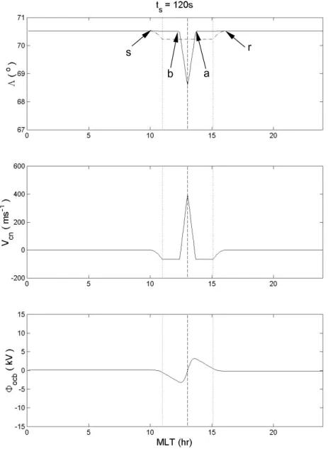
The model presented here is based on the concepts intro-duced by Cowley and Lockwood (1992). The implementa-tion of these concepts is best discussed using Fig. 4 which shows some output data produced by the model. In Fig. 4a, the solid line shows the latitude of the OCB, 3OCB, as a

func-tion of MLT; the dot-dashed line shows the latitude of the

equilibrium boundary location, 3E. Both of these are for

a certain time (in this case ts = 120 s into the simulation).

Because the equilibrium boundary is for the amount of open flux present at that time, the total magnetic flux poleward of these two boundaries must, by definition, be equal at all times: because the ionospheric field is approximately con-stant at Bi =5×10−5T, this means that the area poleward of

the two boundaries must always be the same. Once the loca-tions of these two boundaries is known as a function of MLT, we can evaluate the velocity of poleward motion of the OCB which, in the absence of any reconnection, is taken always to be relaxing towards the equilibrium boundary with a

char-acteristic time constant of τOCB. In general, we could take

τOCB to be a specified function of MLT, however, in this

pa-per, we use as simpler formulation with τOCBset at a constant

value of 10 min at all MLT. This value is taken from analysis of the EISCAT-AMPTE data discussed in Sect. 1.2. Taking the time derivative yields the poleward convection velocity caused by the boundary motion:

Vcn(MLT, ts) = p ×[3E(MLT, ts)−

3OCB(MLT, ts)] /τOCB(MLT), (3)

where p is the distance in the poleward direction correspond-ing to a unit difference in invariant latitude (here we use the value for a height h of 300 km and thus p is equal to

(RE +h) ×2π/360 = 116 km for 3E and 3OCB in

de-grees). This convection velocity will, in general, differ from

the poleward boundary velocity Vbn because reconnection

may be present:

Vbn(MLT, ts) = Vcn(MLT, ts) − V0(MLT, ts), (4)

where V0 is the convection velocity, poleward across the

OCB in the OCB rest frame. Thus V0 is zero at the MLT

1

b a

r s

Fig. 4. Output model data for simulation time ts =120 s and as a function of MLT. (a) The latitude of the (solid line) open-closed field line boundary (3_OCB)and (dot-dashed line) the equilibrium boundary location (3_E). (b) The poleward convection velocity at the OCB, Vcn. (c) The electrostatic potential around the open-closed boundary 8OCB. In each panel, the vertical dashed line is the centre of the merging gap and the vertical dotted lines mark the ends of the merging gap (a and b) for its maximum extent.

for a merging gap which maps to a magnetopause recon-nection site where open flux is generated and V0<0 for all MLT which map to a tail reconnection site. To allow for the fact that a merging gap, corresponding to a reconnection

X-line of fixed MLT extent becomes slightly longer when the

boundary erodes equatorward, a small correction is made

V0(MLT, ts) =

V_o0(MLT, ts) ×cos[3OCB(MLT, ts)]/cos[3i], (5)

where 3i is a reference boundary invariant latitude. We

use the value of 3OCB at the start of the simulation

and adopt a polar cap which is initially circular and thus

3OCB(MLT ,0) = 3i. As will be discussed in the Sect. 3,

the variation of V_o0is specified as a function of MLT and

sim-ulation time ts by the tail and magnetopause reconnection

variations which are inputs to the model. Thus application of Eqs. (3), (4) and (5) allows us to evaluate both the latitudinal

convection velocity (positive poleward) Vcn, and the

bound-ary motion velocity (again positive poleward) Vbn, both as a

function of MLT and time ts.

The boundary velocity Vbnis used to update the polar cap

boundary location at each MLT for the next time step of the simulation 1ts later:

3OCB(MLT, ts+1ts)

The velocity Vcn corresponding to the boundary locations

shown in Fig. 4a is presented as a function of MLT in Fig. 4b: because Vcn =ET/B, this specifies the distribution of

elec-tric field tangential to the boundary, ET, and the ionospheric

potential around the polar cap boundary, 8OCB, by

integrat-ing with respect to the angle ϕ (which corresponds to MLT) we derive the potential as a function of MLT for the time ts

8OCB(MLT, ts) =

Z ϕ 0

Vcn(MLT, ts)Bi(RE+h)cos[3OCB(MLT,ts)]dϕ. (7)

We define the angle ϕ to be positive toward dusk (see Fig. 3a) and to be the angle subtended at the centre of the polar cap by the centre of the reconnection merging gap and the MLT meridian in question. The distribution of potential around the OCB shown in Fig. 4c is typical of observations (Lu et al., 1989) and is used to find the potential distribution through-out the polar cap and auroral oval by assuming ionospheric conductivity is independent of position and solving Laplace’s equation. We simplify this calculation here with the

approx-imation that the OCB is circular (at 3 = 3o) as this allows

the equations given by Freeman et al. (1991) to be applied (see their Appendix A). After taking F , the Fourier

trans-form of 8OCB(MLT, ts)) sampled using N points (24/N ) h

apart in MLT, we evaluate the coefficients amand bmfrom:

m >0, am= −2I {F (m + 1)}/N

m =0, am=0 (8)

m >0, bm=2R{F (m + 1)}/N,

m =0, bm=F (1)/N, (9)

where R{F } and I {F } are the real and imaginary parts of

F. To allow us to use a fast digital Fourier transform here,

we adopt N = 256. The solution to Laplace’s equation is facilitated by replacing latitude by a parameter x:

x =log_e{tan([(π/2) − 3]/2)}, (10)

which has a value xoat the circular convection boundary at

3 = 3o. Different equations apply to the convection polar

cap (3≥3o) and the convection auroral oval (3≤3o). The

value of 3o used is the latitude at the ends of the merging

gap (the points a and b in Fig. 3). Outside of the bulge on the OCB between a and b, the actual OCB in the

simula-tion presented here is rarely more than 1◦(corresponding to

p = 116 km) from this idealised circular boundary and the

error introduced by using a circular convection boundary is small. Inside the polar cap bulge, caused by erosion between

a and b, the flow is taken to be poleward at speed Vcn and

equatorward of the bulge region, the sunward flow stream-lines are shifted equatorward by the thickness of the bulge at that MLT. This ensures that streamlines are continuous across the OCB.

Inside the convection polar cap 3≥3o, the potential 8 is

determined from:

d8/dx = 6mmem(x−xo)[amsin(mϕ) + bmcos(mϕ)], (11)

d8/dϕ = 6mmem(x−xo)[amcos(mϕ) − bmsin(mϕ)] (12)

and the northward and eastward flow velocities, respectively

VNand VEfrom

VN = −{d8/dϕ}/{Bi(RE+h)sin[(π/2) − 3]} (13)

VE = −{d8/dx}/{Bi(RE+h)sin[(π/2) − 3]}. (14)

In the convection auroral oval (3≥3≥31) the convection

pattern is restricted to poleward of a latitude 3 = 31which,

by Eq. (10), corresponds to x = x1. In the present

simula-tion, a fixed value of 31=65◦is employed: this is the

lati-tude of the region 2 ring of field-aligned current. To accom-modate the bulge in the OCB at the merging gap, a new pa-rameter x0_{(ϕ)is used. Outside the merging gap (ϕ}

a<ϕ<ϕb),

x0(ϕ)is the same as x, as given by Eq. (10). Inside the merg-ing gap (ϕ<ϕa and ϕ>ϕb) we introduce a latitudinal shift

equal to the latitudinal separation of the OCB and the con-vection boundary at that MLT, giving a modified latitude,

30(ϕ) = 3 + {3o(ϕ) − 3OCB(ϕ)}: ϕa< ϕ < ϕb:x0(ϕ) = x ϕ < ϕa and ϕ > ϕb: x0(ϕ) =log_etan([(π/2) − 30(ϕ)]/2) (15) d8/dx0=6mm[cosh{m(x0−x1)}]/sinh m(xo−x1)]× [amsin(mϕ) + bmcos(mϕ)] (16) d8/dϕ = 6mm[sinh{m(x0−x1)}/sinh{m(xo−x1)}]× [amcos(mϕ) − bmsin(mϕ)]. (17)

The northward and eastward flow velocities, respectively VN

and VE, are derived from

3 < 3OCB & 3 < 3o: VN= −{d8/dϕ}/{Bi(RE+h)sin[(π/2) − 30]} 3o> 3 ≥ 3OCB: VN=Vcn. (18) 3 < 3OCB & 3 < 3o: VE= −{d8/dx}/{Bi(RE+h)sin[(π/2) − 30]} 3o> 3 ≥ 3OCB: VE=0. (19)

The condition 3o>3≥3OCB only applies in the bulge of

newly-opened flux equatorward of the merging gap ab, where the flow is taken to be uniformly poleward (i.e. with the con-vection velocity at the merging gap).

Thus the model can generate the full convection pattern once the variation of the actual and equilibrium boundary lat-itudes with MLT has been evaluated. To do this, we use the concepts described schematically in Fig. 3 and the points r and s, sunward of which the equilibrium boundary is per-turbed equatorward by the reconnection pulse, which mi-grates towards midnight; this motion reflects the tailward evolution of the newly-opened flux produced by the

recon-nection pulse. For example, the points r and s are at ϕ = ϕr

and ϕ = ϕs and are initially placed at a and b at the start

of the reconnection pulse, moving longitudinally at angu-lar velocities dϕr/dts and dϕs/dts = −dϕr/dts,

respec-tively, (such that r and s both travel at the same speed to-ward the nightside, around the dusk and dawn flanks, respec-tively). This angular speed is an input to the model.

Al-though dϕr/dts could, in general, be a function of MLT, we

here adopt a constant value of 0.25◦_s−1 _{(corresponding to}

1 h of MLT per min). Thus the expansion takes 12 min to propagate to all MLT. The rate of equatorward motion of the equilibrium boundary at a given MLT is controlled by the re-connection rate history. From this we define a propagation time, 1tϕ, from the ends of the merging gap a and b for each

MLT. Outside the merging gap on the duskside, π >ϕ > ϕa

1tϕ =(ϕ − ϕa)/|dϕr/dts|. (20)

Outside the merging gap on the dawnside, π <ϕ<ϕb

1tϕ =(ϕb−ϕ)/|dϕr/dts|. (21)

Inside the merging gap ϕ<ϕaand ϕ>ϕb

1tϕ =0. (22)

Using this propagation delay we can update the equilibrium boundary latitude at each MLT using the reconnection rate history:

3E(MLT,ts+1ts) = 3E(MLT , ts)+

k(ts) × 1ts ×Vo0(ϕ =0, ts−1tϕ), (23)

where V_o0(ϕ =0, ts−1tϕ)is the ionospheric velocity

corre-sponding to the reconnection rate at the centre of the merg-ing gap at the time 1tϕearlier. The normalising constant k is

evaluated at each time tsto ensure that the total magnetic flux

poleward of the equilibrium boundary is always the same as

the polar cap open flux Fpc (poleward of the OCB) at the

same time.

The polar cap flux Fpcis updated using:

Fpc(ts+1ts) = Fpc(ts)+

1tsBi(RE+h)cos(3o)

Z 2π 0

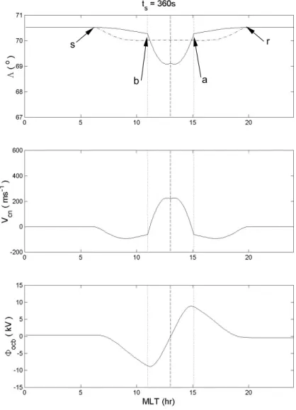
V_o0(ϕ)dϕ. (24) This scheme for evolving the OCB and equilibrium bound-aries is demonstrated by comparing Figs. 4 and 5. Figure 5 is the same as Fig. 4, but for a later time of ts =360 s. It can be

seen, in Fig. 5a, that the points r and s have evolved towards the nightside and that the erosion of the OCB towards lower

latitudes has continued in the merging gap ab which has ex-panded in length. Outside the merging gap, between s and b and between a and r, the evolution of the OCB towards the equilibrium boundary can be seen to have begun. Figures 5b and c show that the flow speeds and convection voltage have also increased.

In implementing the model presented here, we only con-sider changes and boundaries after information about them has arrived in the ionosphere; this removes the need to

spec-ify the Alfv´en wave propagation time, tA, along the field

lines from the reconnection site. (Therefore, in applications where the reconnection rate is specified using input IMF data from an upstream interplanetary monitor, this propagation

time, tA, should be added to the satellite-to-magnetopause

travel time). In the simulation presented here, the flow

across the merging gap, V_o0, begins to increase at ts = 60 s

(see Sect. 3) and thus the magnetopause reconnection com-menced at ts =60 − tA. To be consistent, we have to define

the polar cap flux Fpc to be the open flux of which the iono-sphere has “knowledge”–which was the open flux threading the magnetopause at a time tAearlier.

Note that the model does not require us to define where open field lines are generated on the magnetopause – other than the MLT of the reconnection X-line footprints in the ionosphere must be specified, which is done by the input re-connection rate variation specification, V0

o(ϕ, ts). Thus there

is no assumption of either component or anti-parallel recon-nection. In principle, there may be additional effects relating to the time it takes for newly-opened flux to evolve into the tail from different reconnection sites; however, proper evalu-ation would also require specificevalu-ation of the sheath flow over the whole of the reconnecting magnetopause which requires global MHD modelling. These effects would be a perturba-tion to the simple concept of the expansion of the equilibrium boundary perturbation used here, away from noon at an an-gular speed dϕr/dts.

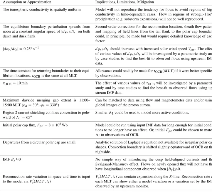
The model contains a number of simplifications and as-sumptions which have been discussed in this section as they arose. Table 1 collects these assumptions together and gives a brief analysis of the implications and limitations that each sets and any mitigating steps that can be used to reduce the uncertainties they cause.

3 An example input reconnection scenario

In order to run the model, the reconnection rate behaviour in space and time must be specified as an input. This is done by prescribing the ionospheric flow velocity V0_{(MLT, t}

s)across

the OCB in its own rest frame. To remove complications caused by the length of the merging gap ab changing with latitudinal motions, we specify the corresponding velocity

V0(MLT, ts)for a hypothetical boundary at constant latitude

3oand then use Eq. (5).

In the discussion of the physical basis of the model, the reconnection rate variation (in space and time) that adds up to a pulse of magnetic flux transfer across the merging gap

Table 1. Summary of assumptions and approximations

Assumption or Approximation Implications, Limitations, Mitigation

The ionospheric conductivity is spatially uniform Model will not reproduce the tendency for flows to avoid regions of high conductivity in time-dependent cases. Flow in regions of strong,>1 keV precipitation (e.g. substorm expansions) will not be well reproduced. The equilibrium boundary perturbation spreads from

noon at a constant angular speed of |dϕr/dts|on both dawn and dusk flank

Second-order corrections for the reconnection location, sheath flow pattern and mapping of field lines from the tail flank to the polar cap boundary could, in principle, be made but would require detailed knowledge of each factor.

|dϕr/dts| =0.25◦s−1 dϕr/dts should increase with increased solar wind speed Vsw. The effect of various values of dϕr/dtswill be investigated by a parametric study and by case studies to find the best-fit to observed flows using upstream IMF data.

The time constant for returning boundaries to their equi-librium locations, τOCBis the same at all MLT.

Allowance could readily be made for τ_OCB(MLT )if it were better specified by observations.

τ_OCB=10 min The effect of various values of τ_OCBwill be investigated by a parametric

study and by case studies to find the best-fit to observed flows using up-stream IMF data.

Maximum dayside merging gap extent is 11:00– 15:00 MLT (ϕa=30◦; ϕb=330◦)

Can be matched to data using flow and magnetometer data and/or using global images of the proton aurora.

Region 2 current shielding confines convection to pole-ward of 31=65◦

Smaller 31could be used to model more active conditions.

Initial polar cap flux, Fpc=8 × 108Wb Model could be run using input IMF data for long enough for initial condi-tions to no longer have an effect. Or, initial Fpccould be chosen to match

3ito observations of OCB.

Departures from a circular polar cap are small. Analytic solution of Laplace’s equation not available for irregular polar cap shapes. Convection boundary is shifted slightly equatorward of OCB on the nightside.

IMF By≈0 No simple way of introducing the cusp field-aligned currents and the

Svalgaard-Mansurov effect. Flows on newly opened flux will not have the have longitudinal component observed when |By|0.

Reconnection rate variation in space and time is input to the model via V_o0(MLT , ts)

V_o0(MLT , ts)can contain expansion along the X-line. Reconnection rate at each MLT can show either a model variation or a variation set by the IMF observed by an upstream monitor.

abwas considered in general terms and not specified. In the

simulation presented here, the reconnection takes place at a single magnetopause X-line AB, the merging gap of which

abis centred at 13:00 MLT (corresponding to ϕ = 0) and

which has a maximum extent of 11:00–15:00 MLT (i.e. a

is at 15:00 MLT and so ϕa = 30◦; b is at 11:00 MLT and

ϕb =330◦). The simulation commences with a pre-existing

open flux of FP C = 8 × 108Wb. Each reconnection pulse

starts at the X-line centre and expands towards both dusk and dawn (to a and b, respectively) at a rate (d|ϕX|/dts)

which we set to 0.167◦s−1, corresponding to 1 h of MLT per 1.5 min. Similarly, the end of each reconnection pulse is first seen at 13:00 MLT, δt = 1 min after the onset, and propa-gates towards both a and b at the same rate. Thus each pulse causes the reconnection to be active at any MLT between a

and b for one minute. Two such pulses are included in the present simulation, with onsets at ts =1 min and ts =9 min.

The background reconnection rate outside the two pulses is taken to be zero.

At the centre of the X-line, the reconnection rate within the pulses is such that, over the repetition period of τ = 8 min, the average poleward convection speed produced would be

V_x∗ = 500 ms. This means, because V_o0is always zero

out-side the pulses, that V_o0 = V_x∗×(τ/δt )within them at the centre of the X-line. Lastly, the amplitude of the pulses is decreased to zero as they approach a and b. This is neces-sary to avoid discontinuities in the OCB forming at a and b. We here employ a cosinusoidal decrease with distance away

1

b a

r s

Fig. 5. Same as Fig. 4, but for simulation time ts=360 s.

from the centre of the merging gap: for ϕ < ϕa: Vo0(ϕ, ts)=

(ϕ, ts) × Vx∗×(τ/δt ) ×cos{(π/2) × (ϕ/ϕa)}

for ϕ > ϕb: Vo0(ϕ, ts)=(ϕ, ts) × Vx∗×

(τ/δt ) ×cos{(π/2) × (|2π − ϕ|/|2π − ϕb|)}, (25)

where (ϕ, ts)is equal to unity for a time ts for which the

ϕconsidered is inside a propagating reconnection pulse and

equal to zero at all other times, as prescribed above.

This specification of the reconnection behaviour, as a

function of simulation time ts and MLT, is the input to

the convection model described in the previous section. Each pulse in this example causes the open flux to

in-crease by 0.185×108Wb in total. At the start of the

simulation presented here, the pre-existing open flux is

Fpc =8.00×108Wb, rising to 8.185×108Wb at the end of

the first pulse and 8.37×108Wb at the end of the second;

thus each pulse adds ∼ 2.3% to the polar cap.

4 Results

Figure 6 demonstrates the presentation format of the model output. The top panel shows the variation with simulation time ts of two key voltages: the blue line gives the

reconnec-tion voltage 8XLproduced by the input scheme discussed in

the previous section, the red line shows the polar cap voltage

8P C that results from the convection model. The voltage

8XLis total instantaneous voltage that exists along the

day-side ionospheric merging gap in its own frame of reference. Note that 8XLhas been divided by a factor of 5 to enable

dis-play on the same scale as 8P C. The vertical green line marks

the tsof the convection pattern shown in the lower panel (the

example presented in Fig. 6 is for ts =660 s). Under the top

panel the current values of 8P C and 8XL are given in red

and blue text, respectively.

The reconnection voltage, 8XL, shows the input of two

pulses to this simulation. The prescribed motion of the

square-wave reconnection rate pulses and the cosinusoidal

0 450 900 1350 1800 0 20 40 t s = 660s ΦPC ΦXL/ 5 kV Φ_PC = 28 kV Φ XL = 115 kV F PC = 8.32 x 108 Wb ∆Φ = 3 kV 60 deg 12 MLT = 0hrs 18 6

Fig. 6. An example of the output from the model. The top panel gives the variation with ts of 8XL/5 , where 8XLis the input re-connection voltage (in blue) and of the resulting transpolar voltage

8P C (in red). The vertical green line gives the simulation time

ts of the convection pattern shown in the MLT-invariant latitude

(3)plot beneath. In this lower plot, 12:00 MLT is to the top and 06:00 MLT to the right and the outer circle is 3 = 60◦. Adiaroic (non-reconnecting) segments of the OCB are shown in black, re-connecting segments of the OCB in red. Equipotential contours,

18 =3 kV apart, are shown in blue. The green lines delineate flux opened by the two reconnection pulses. The current values of the voltages 8XLand 8P Cand of the polar cap flux Fpc are given in blue, red and mauve text, respectively.

shown, with a steep rise after the onset of each pulse

fol-lowed by a slower decay. The peak 8XL in each pulse is

about 150 kV. The polar cap voltage 8P C is the difference

between the maximum and minimum potential produced in the ionosphere. The red line shows that this increases during each reconnection pulse but decays slowly after the pulse. In the simulation presented here, with the pulses 8 min apart, the flow voltage due to the first pulse has already peaked near 20 kV but only decayed fractionally from this peak when the

second pulse occurs and raises 8P C to above 35 kV. At the

end of the simulation, at ts = 1800 s, 8P C has decayed to

about 5 kV.

The lower part of Fig. 6 gives, in blue, the convection

streamlines at the ts shown. The separation of the

stream-lines shown is 18 = 3 kV in all cases shown here. In this plot, 12:00 MLT is to the top, 06:00 MLT to the right and 18:00 MLT to the left. The outer black circle gives the lati-tude 3 = 60◦, but flow is confined to poleward of 31=65◦

(effectively the latitude of the region 2 ring). The OCB is shown in black where it is adiaroic and in red where recon-nection is active (V0>0). The green lines delineate the field lines opened during the two reconnection pulses. The value of the open flux FP Cis given in the bottom left in mauve.

Several features can be noted in this example. Firstly, the convection reversal boundary lies equatorward of the OCB

at all MLT outside the merging gap. This is an artefact of the model and results from the use of a simplifying circular

convection boundary which gives 3o<3OCB at these MLT.

Two active reconnecting (V0>0) segments of the OCB can

be seen at this tswhich are propagating away from the centre

of the merging gap (13:00 MLT); in this case they are part of the second of the two input reconnection pulses.

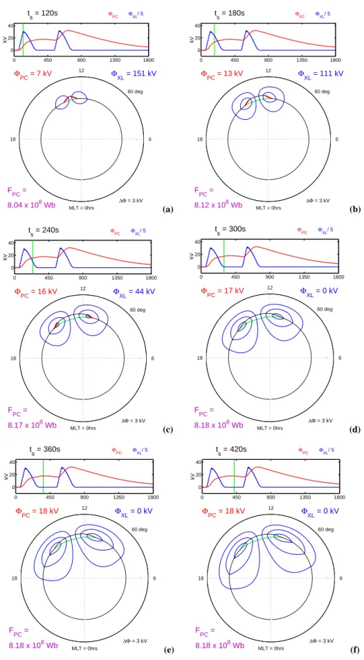
Figure 6 is one frame in a sequence of patterns which

is summarised in Fig. 7. Figure 7a is for ts = 2 min,

one min after the Alfv´en wave launched by the reconnec-tion onset reached the ionosphere: a number of features can be observed. The effects of the active reconnection seg-ments (in red) can be seen in the equatorward erosion of the OCB that it has caused. The reconnection voltage, the total rate of flux transfer into the open field line region, is

8XL=171 kV at this time, whereas the polar cap flow

volt-age is just 8P C =7 kV (thus, just two flow streamlines can

be seen in Fig. 7a in the localised vortices because a contour separation of 18 = 3 kV is employed). The large

differ-ence between 8XLand 8P Cis because, initially, the

recon-nection pulse predominantly causes equatorward erosion of the OCB within the merging gap rather than poleward con-vection. At the very centre of the bulge of newly-opened flux, the signature of the switch-off of the reconnection can be seen in Fig. 7a, having just begun and causing the ap-pearance of an adiaroic boundary segment at 13:00 MLT.

Figure 7b is for ts = 3 min and both the signatures of

on-set and switch-off of the reconnection have moved away from 13:00 LT towards both dawn and dusk. This azimuthal motion of the region of active reconnection is as proposed and deduced from observations by Lockwood et al. (1993a), Lockwood (1994), Smith and Lockwood (1996), Milan et al. (2000) and McWilliams et al. (2001). The flow pattern

has enhanced (8P C = 13 kV ), even though the

reconnec-tion voltage has begun to decrease (8P C = 111 kV). The

flow pattern has expanded spatially towards both dawn and dusk. This early expansion reflects a mixture of the expan-sions of both the active merging gap and of the disturbance

to the equilibrium boundary. The changes seen between

Fig. 7a and b all continue until ts = 9 min when the

sec-ond reconnection pulse commences. When ts =10 min, this

second pulse has produced a second equatorward erosion of the OCB, almost identical to the first. However, Figs. 7h–6j

(ts =10 − 12 min) show a convection response to the second

pulse that is considerably different to the first, in that the re-sponse is not localised and expanding but has elements of a global instantaneous response. The transpolar voltage peaks at 8P C=32 kV at ts =12 min, just before the reconnection

voltage due to the second pulse decays to zero. Subsequently, the convection pattern decays in a shape-preserving manner with potential contours migrating towards the OCB at dawn and dusk where they disappear. This is illustrated by compar-ison of Figs. 7j, k and l, for ts of 12 min, 16 min and 20 min,

respectively.

Note that the boundary erosion predicted by the model, due to each pulse, is of order 1 − 2◦of latitude (see Figs. 4, 5 and 7), corresponding to 116–232 km. This is consistent with

0 450 900 1350 1800 0 20 40 t s = 120s ΦPC ΦXL/ 5 kV Φ_PC = 7 kV Φ XL = 151 kV F PC = 8.04 x 108 Wb ∆Φ = 3 kV 60 deg 12 MLT = 0hrs 18 6 (a) 0 450 900 1350 1800 0 20 40 t s = 180s ΦPC ΦXL/ 5 kV Φ_PC = 13 kV Φ XL = 111 kV F PC = 8.12 x 108 Wb ∆Φ = 3 kV 60 deg 12 MLT = 0hrs 18 6 (b) 0 450 900 1350 1800 0 20 40 t s = 240s ΦPC ΦXL/ 5 kV Φ_PC = 16 kV _Φ XL = 44 kV F PC = 8.17 x 108 Wb ∆Φ = 3 kV 60 deg 12 MLT = 0hrs 18 6 (c) 0 450 900 1350 1800 0 20 40 t s = 300s ΦPC ΦXL/ 5 kV Φ_PC = 17 kV _Φ XL = 0 kV F PC = 8.18 x 108 Wb ∆Φ = 3 kV 60 deg 12 MLT = 0hrs 18 6 (d) 0 450 900 1350 1800 0 20 40 t s = 360s ΦPC ΦXL/ 5 kV Φ_PC = 18 kV Φ XL = 0 kV F PC = 8.18 x 108 Wb ∆Φ = 3 kV 60 deg 12 MLT = 0hrs 18 6 (e) 0 450 900 1350 1800 0 20 40 t s = 420s ΦPC ΦXL/ 5 kV Φ_PC = 18 kV Φ XL = 0 kV F PC = 8.18 x 108 Wb ∆Φ = 3 kV 60 deg 12 MLT = 0hrs 18 6 (f)

Fig. 7. Selected output convection patterns, each frame using the same format as Fig. 6. Note that the frames are not equally spaced in simulation time, ts.

0 450 900 1350 1800 0 20 40 t s = 540s ΦPC ΦXL/ 5 kV Φ_PC = 16 kV Φ XL = 0 kV F PC = 8.18 x 108 Wb ∆Φ = 3 kV 60 deg 12 MLT = 0hrs 18 6 (g) 0 450 900 1350 1800 0 20 40 t s = 600s ΦPC ΦXL/ 5 kV Φ_PC = 20 kV Φ XL = 159 kV F PC = 8.23 x 108 Wb ∆Φ = 3 kV 60 deg 12 MLT = 0hrs 18 6 (h) 0 450 900 1350 1800 0 20 40 t s = 660s ΦPC ΦXL/ 5 kV Φ_PC = 28 kV Φ_XL = 115 kV F PC = 8.32 x 108 Wb ∆Φ = 3 kV 60 deg 12 MLT = 0hrs 18 6 (i) 0 450 900 1350 1800 0 20 40 t s = 720s ΦPC ΦXL/ 5 kV Φ_PC = 32 kV Φ XL = 45 kV F PC = 8.37 x 108 Wb ∆Φ = 3 kV 60 deg 12 MLT = 0hrs 18 6 (j) 0 450 900 1350 1800 0 20 40 t s = 960s ΦPC ΦXL/ 5 kV Φ_PC = 24 kV _Φ XL = 0 kV F PC = 8.37 x 108 Wb ∆Φ = 3 kV 60 deg 12 MLT = 0hrs 18 6 (k) 0 450 900 1350 1800 0 20 40 t s = 1200s ΦPC ΦXL/ 5 kV Φ_PC = 17 kV _Φ XL = 0 kV F PC = 8.37 x 108 Wb ∆Φ = 3 kV 60 deg 12 MLT = 0hrs 18 6 (l) Fig. 7. Continued.

1

b a r1

s1

s2 r2

Fig. 8. Same as Fig. 4 but for simulation time ts =660 s. Note that the vertical axes scales are expanded compared to those used in Figs. 4 and 5.

the equatorward motions of the boundary seen during tran-sient events by ground-based radars and optical imagers (e.g. Lockwood et al., 1993a, b; Milan et al., 2000) and space-based proton aurora imagers (Lockwood et al., 2003). It is also consistent with the separation of cusp ion step signa-tures seen by both low and middle altitude spacecraft (e.g. Lockwood and Davis, 1996).

5 Discussion

The results presented in the previous section reveal some in-teresting features of the convection response to reconnection pulses and, in particular, how that response depends upon the pre-existing flow that remains following prior reconnec-tion activity. The principles behind this can be understood from Fig. 8, which is the plot equivalent to Fig. 4, but for

simulation time ts = 660 s corresponding to Fig. 7i. The

top panel shows the latitudes of the OCB and the equilibrium

boundaries (3OCBand 3E); the effects of both of the

recon-nection pulses can be seen in both boundaries. The perturba-tion to the equilibrium boundary, caused by the first pulse,

has reached 24:00 MLT on the dusk side (r1) and almost

1:00 MLT on the dawnside (s1). Thus, this perturbation due

to the first pulse is close to encircling the entire polar cap, after which the flow would have, in the absence of the sec-ond pulse, decayed exponentially in a quasi shape-preserving manner. However, the perturbation due to the second pulse

can be seen emerging from the merging gap (with r2

propa-gating east, away from a, and s2propagating west away from

b). The effect of the first pulse can be seen in the OCB lati-tude by the fact that it has moved equatorward at MLTs out-side the merging gap (except near midnight, where neither

3E nor 3OCB has yet to be influenced). The effect of the

second pulse can be seen as a large equatorward migration within the merging gap ab. The two pulses can be identified in the poleward convection speeds, with equatorward motion

mid-night) and strong poleward flow (Vcn>0) inside the merging

gap. An enhancement of the equatorward flow is seen just

outside of the merging gap (between a and r2and between

b and s2) but this is much weaker than the poleward flow

between a and b. This should be contrasted with the situa-tion for the equivalent time following the first pulse where

the total equatorward flow (between a and s1and between

band r1) matches the total poleward flow between a and b.

Indeed, in the bottom panel of Fig. 8 it can be seen that the

additional equatorward flow between a and s2and between b

and r2causes only a very small perturbation to the potential

distribution around the OCB.

The important point is that, at s2 and r2, the OCB and

the equilibrium boundaries are close together, such that

|3OCB−3E|is small and thus Vcnis near zero. This

situa-tion arises because the equilibrium boundary at these MLTs is perturbed equatorward by the second pulse, while the OCB has been perturbed equatorward by a similar amount by the first pulse. This means that the flow streamlines that flow poleward into the polar cap between a and b flow back

equa-torward across the OCB, not sunward of s2and r2, as would

have been the case without the prior reconnection pulse, but closer to midnight. Near s2 and r2 at this ts, the flow that

would have been caused by the first pulse in isolation is poleward whereas that which would be caused by the sec-ond pulse in isolation would be equatorward and compara-ble in magnitude. Thus they almost completely cancel each other out. The net effect is that the flows due to the two pulses add to form the flow pattern given in Fig. 7i, which shows enhancement at all MLT (except near midnight) in re-sponse to the second reconnection pulse. Thus the rere-sponse is much more global in nature than it was for the first pulse. A full analysis and comparison of the expanding and quasi-global responses will be presented in a later paper (Morley and Lockwood, 2003).

The two reconnection pulses in the sequence simulated here are identical and the differences in the response of the second pulse are entirely due to the remnant effects of the first pulse. Thus this example, for the first time, highlights the importance of the reconnection history in determining the response to a given reconnection voltage change. This fac-tor has not previously been considered and may offer an ex-planation of the different convection responses to southward turnings of the IMF that have been reported in the literature (see Sect. 1.2). Indeed, Fig. 7 suggests that the response to the second pulse is more instantaneous in nature, whereas that following the first pulse is clearly expanding in nature. This possibility will be investigated in detail in a follow-up publication.

6 Applications of the model

The numerical model presented here has many applications, beyond the studies of the convection response to reconnec-tion rate variareconnec-tions, of which we have presented just one ex-ample. In this paper we have concentrated on variations in

the dayside magnetopause reconnection rate. This case is relatively simple because the associated precipitation in the cusp is relatively soft and conductivity changes are not as important a factor as they are on the nightside where precip-itation has higher energies. The model presented here does not include spatial structure in the ionospheric conductivities and, in general, these will influence the pattern of convection. Allowance for this would require a much more complex al-gorithm than is used here to convert the potential distribution around the OCB into an equipotential map of everywhere poleward of the region 2 field-aligned current ring. However, extensions to the model which made allowance for the spa-tial and temporal variations of precipitation would improve the realism of the model and would increase the number of applications.

Conductivity structure and variations become a highly rel-evant factor when discussing the nightside and, in particular, the phenomenon of substorms. For computing the potential distribution around the OCB, the model can readily be gener-alised to include nightside reconnection in the cross-tail cur-rent sheet. However, the precipitation associated with sub-storms generates conductivity structure which varies rapidly at substorm onset.

For the dayside reconnection phenomena, a large number of studies are made possible by the model in its present form, because precipitation down newly-opened field lines gener-ates a number of signatures and the nature of those signa-tures depends on how those field lines are moved by convec-tion. Examples of this type of application include modelling cusp ion steps, cusp proton aurora bursts seen by global im-agers, poleward-moving events seen by incoherent and co-herent scatter radar, polar cap patches, red-line auroral tran-sients and dayside ion heating events. In addition, in a fu-ture paper, we will apply the model to investigate the various methods that have been applied to observations to determine the rate of expansion of the flow pattern.

Acknowledgements. The authors thank Mervyn Freeman of British

Antarctic Survey for many helpful discussions and to B.S. Lanch-ester of the University of Southampton for helpful discussions, proof reading and support. This work was supported by the UK Particle Physics and Astronomy Research Council.

Topical Editor M. Lester thanks two referees for their help in evaluating this paper.

References

Banks, P. M., Araki, T., Clauer, C. R., St-Maurice, J. P., and Fos-ter, J. C.: The interplanetary magnetic field, cleft currents, and plasma convection in the polar caps, Planet. Space Sci., 32, 1551–1560, 1984.

Clauer, C. R. and Banks, P. M.: Relationship of interplanetary elec-tric field to the high latitude ionospheric elecelec-tric field and cur-rents: observations and model simulation, J. Geophys. Res., 93, 2749–2754, 1988.

Cowley, S. W. H.: Solar wind control of magnetospheric con-vection, in: Achievements of the international magnetospheric