Econometric model of ski resort real estate in New England

ECONOMETRIC MODEL OF SKI RESORT REAL ESTATE IN NEW ENGLAND

by

William Daniel Gause Master of Engineering Cornell University, 1988

Bachelor of Science Cornell University, 1987

SUBMITTED TO THE DEPARTMENT OF ARCHITECTURE

IN PARTIAL FULFILLMENT OF THE REQUIREMENTS OF THE DEGREE MASTER OF SCIENCE IN REAL ESTATE DEVELOPMENT AT THE

MASSACHUSETTS INSTITUTE OF TECHNOLOGY SEPTEMBER, 1993

@ William Daniel Gause 1993 All rights reserved

The Author hereby grants to M.I.T.

permission to reproduce and to distribute publicly copies of this thesis document in whole or in part.

Signature of the author_________________

William D. Gause Department of Architecture July 31, 1993 Certified by William C. Wheaton Professor of Economics Thesis Supervisor Accepted by William C. Wheaton Chairman Interdepartmental Degree Program in Real Estate Development

RatctIl

MASSACHUSETTS INSTITUTE

OF TFCANOLQGy

OCT 0 4 1993

ECONOMETRIC MODEL OF SKI RESORT REAL ESTATE IN NEW ENGLAND

by

WILLIAM DANIEL GAUSE

Submitted to the Department of Architecture on July 31, 1993 in partial fulfillment of the requirements for the Degree of Master of Science in

Real Estate Development

This paper is an economic analysis of residential ski resort real estate in New England. In an attempt to understand what economic, geographic, demographic, and

climatological factors influence the price of second homes at ski resorts, predictive models were generated for skier visits, condominium rental rates, hotel rental rates, condominium

prices and construction completion rates. These models are based on data collected at a single New England ski resort recognizing that most large New England ski resorts are similar and yet are characteristically different from large Western resorts. This data was collected from historical records dating back twenty-five years, covering several booms and recessions.

The primary purpose of the study was to determine what general factors influence second home prices in New England so that developers and investors would be more knowledgeable in making decisions about when and where to build or invest. Specific models were created for the five condominium projects whose data was used, and these models can be used to predict future prices and rates at these specific projects. The trends, however, should hold true for other New England resorts. The skier visit equation should hold true for all large, southern Vermont ski areas since this model was based on data for the entire state.

The results of the study indicate that skier visits are primarily a function of regional employment and snowfall, with increasing significance associated with employment and decreasing significance associated with snowfall. Condominium rental rates are largely a function of skier visits, condominium stock, total regional employment and the previous year's rental rate. Hotel rates are primarily a function of skier visits and the previous year's rate. Interestingly enough, condo rates are more a function of the previous year's skier visits while hotel rates are better correlated with the current year's skier visits indicating that hotels do a better job of estimating future visits while condominiums estimate this year's demand based on last year's demand. Prices are largely determined according to a consumer's model as opposed to an investor's model. Prices are a function of

rates and inflation. This is a useful characterization of the second home market. Condominium completions are primarily a function of the price, rent, stock and employment.

Based on projected employment figures for the next decade and a half, the paper uses the models to make forecasts of the movement in the ski real estate market in New England. With forecasts of slow but positive job growth in New England and the mid-Atlantic states throughout the year 2010, the models indicate a continued slight drop in skier visits and rents over the next couple of years followed by steady, gradual increases through 2010 as employment edges up. Prices have reached their bottom and should climb gradually over the next decade and a half without reaching their mid-eighties highs (in real terms) over this period. Completions should experience a brief surge over the next two years before tapering off for a couple years and then beginning a slow steady climb,

assuming there are no physical or legal impediments to growth. The degree to which these trends occur is, however, entirely dependent upon the level of employment growth in the region. Employment is the common thread which binds the second home market together.

Thesis Supervisor: William C. Wheaton

TABLE OF CONTENTS

Abstract... 2

Introduction... 5

Factors Affecting the Value of Ski Resort Real Estate... 11

M ethodology of Study ... 22

Skier M arket... 38

Rental M arket... 45

Asset M arket... 56

Forecasting for Ski Resort Real Estate ... 76

Conclusions... 110

Appendix... 117

... %,,- x x x

...

...

. ....

...

...

_....

_...

_.

_..

_.

_...

_...

Purpose of Study

The purpose of this thesis is to track and analyze the history of ski resort real estate prices and rental rates over time and to index them to economic, geographic, and atmospheric factors. The intent is to be able to use these models to forecast future skier visits, rental rates, prices and completions. The study was conducted at a single New England ski resort (Killington/Pico Vermont) for the purpose of determining trends in the industry. The specific models and data can only be applied to the Killington area, but the trends can be used to draw parallels to other New England ski resorts and possibly for other New England recreational real estate in general. If it is possible to estimate a surge or drop in real estate prices by following trends in the regional economy this could be invaluable to a real estate owner or investor. The purpose of the study is to analyze and

predict trends in the second home market for recreational developments rather than specifics from one year to the next. If someone is interested in specific models, they should follow this format to conduct a similar study at the specific resort of interest.

Description of New England Ski Resorts

James Branch of Sno-Engineering Inc. has classified ski resorts into four different types according to their size and characteristics'. Type I resorts are large world-class destination resorts that have many amenities and are often built around a city or town. They often have a lot of foreign investment and well-developed real estate. Examples of such resorts include Aspen, Snowmass and Vail. Type II resorts are similar in size to Type I resorts, but they often don't have as many amenities, aren't built around a thriving

IPatrick Philips, Developing with Recreational Amenities: Golf Tennis, Skiing and Marinas (Washington D.C.: Urban Land Institute, 1986), p.

resort village, and don't attract the same amount of foreign investment. Examples include most large New England resorts such as Killington, Sunday River, Mount Snow and Sugarloaf Type III resorts are smaller than Type II resorts and don't have the same amount of associated real estate. Examples would include smaller New England resorts such as Bromley, Mad River Glen, and Shawnee Peak. Finally, Type IV resorts are small local ski areas that are geared towards local skiers and do not have much in the way of real estate development.

Type I resorts are destination resorts that attract visitors from all over the world for extended stays of one week or longer. Branch argues that people investing in real estate at these resorts are older and more interested in the private use of the real estate. They are less concerned with rental income using the property as an investment tool.

Type II resorts are generally more regional. While they draw people for week-long visits, they often do not have commercial airports and service. They are more

dependent on vehicular traffic and rely on large metropolitan areas within driving distance. As such they, they are often the target of weekend visits. According to Branch, people investing in real estate at Type II resorts are more likely to rely on the rental income from the property. They are often younger and may prefer to ski at a variety of different mountains rather than always skiing at the same place.

Type III resorts are often considered weekend ski areas with primarily local patronage during the week. Type IV resorts are often open only at night and on the weekend, catering only to local skiers.

This study looks at Type II resorts in New England. As mentioned above, Type II destination resorts are often dependent upon people driving to the area. Assuming that most people don't want to spend more than about five hours in a car, New England resorts are primarily dependent upon the Boston and New York metropolitan regions. They are obviously exceptions to this rule, but for the purposes of this study it will be assumed that Massachusetts, Connecticut, New York and New Jersey are the primary markets for skiers

who would be interested in investing in ski resort real estate at Killington. Although there are many skiers from Vermont, New Hampshire and Maine, it is assumed that they are not the primary investors in Killington's resort real estate, since they either already live in the area, or are closer to another mountain.

New England ski resorts are characteristically unique. They are often located near small, quaint New England villages. They are usually situated in small mountain ranges (when compared to the Rocky Mountains) and have skiing trails lined with trees (not cliffs, crevasses and couloirs). They are at a lower elevation than western resorts which means more modest snowfall amounts and a dependence on artificial snowmaking. New England ski resorts generally have one season -winter, although some areas are trying to change that. The character of New England resorts is distinctly different from Western or European resorts and hence has different market appeal. The results of this study are intended to be applicable to Type II New England resorts only. An analysis of Western resorts would have to consider a host of different factors.

Types of Ski Resort Real Estate

Residential ski resort real estate consists primarily of single family detached homes i.e. "chalets", and condominium units. Up until the late seventies and early eighties, single family housing was the most common form of ownership, with relatively few

condominium projects. Since then, however, the popularity of condominiums has

skyrocketed. While condominiums do not offer the solitude and privacy of a single family home, they have many features which make them very attractive to second home buyers. The primary attractions are their lower price, ease of renting, and lack of maintenance. Many people with ski resort homes rent them out when not in use to help cover the cost of ownership. Condominiums have similar features and are often listed with a single broker to facilitate renting. Finally, with all the upkeep of a primary home, many people prefer not to deal with twice as many headaches and opt for maintenance free condominiums.

Another increasingly common form of ownership is the timeshare. These are much more affordable than buying a condominium outright and allow the occupant to pay only for the time they use the unit. It offers much more flexibility than owning a single unit since shares may be traded and the person may easily buy shares at more than one resort, giving them variety. It also eliminates an owner's reliance on renting the unit. The

popularity of timeshares may increase in times of financial belt tightening due to their lower cost. The primary disadvantage is their lack of flexibility and their multiple

ownership. Vacation planning has to be coordinated well in advance. Many people in the field expect to see a surge in the demand for timeshares.2

The other primary type of ski resort real estate is commercial. This includes hotels, restaurants, shops, and other places of business. This study will consider the fluctuation of hotel rents as a measure of the demand for accommodations, however, it will be focused on residential real estate and in particular it will be concentrated on

condominiums. It is assumed that the demand for commercial real estate roughly follows the demand for residential real estate. The more people there are living in the area, the greater the commercial demand will be.

The Market for Ski Resort Real Estate

Ski real estate can be thought of in two types of markets--the investment market and the consumer market. Some people buy resort homes for the investment potential while others buy them to use while skiing or relaxing in the country. As will be discussed later, this leads to two different market models with different input factors.

Statistics indicate that the bulk of the skier market is young, with the average skier between 18 and 35.3 The majority of the second home buyer market is over 35, however,

2

"Resorts and Recreation", Urban Land Special Trends Issue (March 1991), pp. 38-39. 3_{Gregg T. Logan and Ann E. Day, "Ski Resort Real Estate Development", Urban Land} (December 1989), p. 37.

and typically an empty-nester or mature family aged 40 to 55.4 A 1990 study found that while people aged 35 to 64 accounted for 50% of all American householders, they accounted for 70% of the recreational property owners in the country.5 According to Logan and Day, today's typical second home buyer wants to retain private use, are less concerned with rental income, want to use the unit in the off-season as well as the

peak-season, and frequently use the property as a means of bringing together extended families. These are people who can afford to purchase a second home after owning a primary residence. They are looking for more and more amenities and are primarily interested in large condominiums and townhouses.6

Given the profile of the typical second home buyer and the demographic composition of the United States, this country may be on the edge of a surge in the demand for second homes in the coming decade as the "baby-boomers" reach this age group. It is important to note, however, that the "baby-boomers" are aging out of the range of the average skier. As these people age and look to buy second homes they are going to be looking for more amenities than just skiing. It will be increasingly important to provide year-round amenities to attract this potentially huge market.

Leanne Lachman, of Schroder Real Estate Associates in New York, predicts a doubling of the demand for second homes over the next decade as the nations first

generation of dual-income couples reaches middle age with discretionary time and money.7 This demand should occur not only in ski homes, but primarily in year round second homes. To cash in on this market, ski resorts will have to offer year round amenities.

4_Ibid.

5_{Judith Waldrop, "Who Owns Recreational Property?", American Demographics (May 1991),} p.49.

6_{Logan and Day, "Ski Resort Real Estate Development", p. 37.} 7_{Susan Bradford, "Second Homes", Builder (February 1991), p. 79.}

Another factor to consider is the changing lifestyles of Americans. As some people have less leisure time they want to spend it more efficiently. This often means taking mini-vacations instead of the traditional one or two week vacations. Given these trends, the demand for second homes located within several hours of the primary home

should surge.8 This in turn may spell good news for New England ski resorts, as fewer people from New York and Boston look to spend a week or two out West and instead spend more weekends at New England resorts.

Literature Review

The bulk of the literature and research dealing with second home and resort developments is qualitative rather than quantitative. There are many articles speculating that a boom in the second home market is about to occur due to the aging "baby-boomers" and the traditional second home buyer's profile. The problem, however, is that most of the literature is based on opinion and reasoning rather than empirical studies. To the best of the author's knowledge, an econometric model of ski resort real estate has never been conducted that looked at the sales and rental history of an established group of real estate and tried to fit that data to economic, geographic, atmospheric and demographic factors over time. If such a study has been conducted, it was not published in a manner that made the results widely accessible. The literature that is accessible has to do with market

potential and expected future opportunities in a very general sense. This paper will attempt to broaden the scope of the literature dealing with the subject.

8_{Diane R. Suchman, "Opportunities for Recreational Developers", Urban Land (February 1991),}

~.0

Overview

Ski resort real estate values are a function of many different variables including economic, atmospheric, geographic and political influences. The issue at hand is whether it is possible to develop an econometric model to accurately forecast what these values will be over time as the input variables change. In developing such a model, some things are easily quantified while others are obviously not. The following discussion is intended to highlight some of the more prominent factors influencing real estate values. Following this discussion, is a description of the specific model developed and the factors considered. National Economy

The national economy clearly has some effect on the value of recreational real estate, however, that effect may be secondary and not direct. The value of ski resort real estate is a function of the economy that fuels the resort. In the case of a national

destination resort such as a "Class I" Western resort, e.g. Aspen or Vail, the visitors are drawn from across the country and hence the national economy may have some direct effect upon skier visits and hence real estate prices. On the other hand, a New England resort draws visitors primarily from New England and the mid-Atlantic states. The

regional economy is what drives the number of skiers visits and the national economy may have only a secondary effect upon the resort prices by affecting the regional economy.

As will be shown by the model, national mortgage rates have only a limited effect on the value of ski resort real estate.

Regional Economy

As mentioned, the number of skier visits to a resort and the price of real estate at a resort is a function of the employment and the economy in the region comprising the skier market. In the case of weekend destination resorts such as those found in New England, this means that the regional economy has a direct effect upon the value of the real estate. As the employment in New York City and Boston drops, this signals a drop in the regional economy. People are less willing to spend money as their disposable income is reduced and are less likely to go skiing. As the number of skiers drops, so does the rent and the value of the resort real estate. When employment increases in these regions, we see the opposite effect.

Local Economy

The same logic as mentioned above holds true for the local economy. In the case of a "Class IV" local ski area, the ski area is dependent upon the local residents for revenue. If the local economy falters, the ski resort will falter as people's discretionary income is reduced. In the case of these local ski areas, however, residential resort real estate is not a factor. The skiers already live in the area and are not going to buy a second home on the mountain.

On the other hand, when we consider a Class II weekend resort, the local economy does not have much of an effect upon the ski area. Rather the local economy is dependent upon the regional economy. As the regional economy falters, fewer people make trips to the ski area which means lower real estate prices and fewer jobs needed in the local economy. This cycle is even more pronounced when we consider a Class I resort. The national economy affects skier visits to the resort which in turn affects the regional

economy and the local economy. This inter-dependence clearly can have both positive and negative effects for the sub-economies.

National Real Estate Cycle

The national real estate cycle is difficult to quantify and analyze. Real estate markets are local and are a function of local supply and demand. The only factors of the national real estate cycle that may have some effect on ski resort prices are the average

mortgage rate and the consumer price index, which combine to yield the real mortgage rate. The rationale would lead one to expect that as the mortgage rate is lowered, more people can afford to buy real estate and the increased demand causes upward pressure on prices. The econometric model was unable to prove this with any significance, and in fact mortgage rates were more often found to have the reverse effect. In general, mortgage rates were found to have limited effect upon real estate prices.

Regional Real Estate Cycle

As mentioned above, real estate markets are local and are a function of local supply and demand. Regional real estate is a function of the stock and demand in that region. If regional prices fall due to increased stock, this should not have a direct effect upon resort prices. If on the other hand, regional prices fall due to lack of demand resulting from lack of employment or income, this should affect resort prices. There is, therefore, no direct correlation between the regional real estate cycle and the prices of ski

resort real estate. They are dependent upon different factors as well as some common factors. This study did not consider the effect of regional real estate cycles on the value of resort real estate. A more comprehensive study might include this data if it could be obtained to see if the two cycles have any correlation.

Local Real Estate Cycle

Resort real estate is clearly a function of the local second home market, which is a function of the local real estate cycle. Supply and demand drive the local market. As supply in the local area increases, prices will drop unless they are offset by commensurate increases in demand. This demand can be brought on by primary or secondary home

buyers since they could both be competing in the same market. It is, however, more probable that resort real estate buyers will be competing in the second home market, since they will have a higher utility associated with a mountainside location than a primary home buyer. They will also be more affluent people transferring wealth from a region with a higher cost of living (a dollar will not be worth as much to them as it will to a local resident).

Stock of Ski Resort Real Estate

From basic economics, it follows that real estate prices are a function of the total stock. The greater the supply of potential choices, the lower the prices of those choices will be assuming constant demand. As demand increases, however, an increasing supply will only mean reduced prices if the supply grows faster than the demand. If the supply keeps pace with the demand, real prices should remain constant (all other things equal). In predicting real estate prices, it is just as important to be able to predict stock as it is to be able to predict demand.

Number of Skier Visits

Real estate rent and prices are a function of skier demand. The more people there are skiing, the more people are going to need accommodations. As will be shown with the model, skier visits are more important for predicting rental rates than they are for

predicting sale prices. A willingness to ski does not necessarily create a willingness to buy.

Ski Resort Characteristics

The individuality of a resort has an obvious effect on the value of real estate. Each resort has its own individual characteristics that add charm to the resort and draw a certain crowd of people. Some amenities are quantifiable and others are not. The addition of a golf course may have a measurable increase in the value of the real estate (the increased

value should more than offset the cost of the golf course) by adding a year-round attraction to the resort and hence increasing the utility.

On the other hand, some amenities effect on real estate can not be quantified. The ambiance of a resort can either draw people or turn them away. It is important for a resort to keep in mind the reason for its success. The owner of Sunday River Ski Resort in Bethel, Maine attributes the phenomenal growth and success of his resort to maintaining an awareness that visitors are there to ski. They demand the best ski terrain, snow conditions and lift access, and Sunday River has responded by continually putting money back into the skiing to make it top notch.9 _{In the mid-eighties, Sugarloaf/USA Ski Resort} in Kingfield, Maine lost sight of this principle and paid the price. They focused more on real estate than on skiing. The lack of ski related capital improvements led to reduced skier visits and hence reduced demand for real estate. Sugarloaf/USA became over built and was forced to enter Chapter 11 bankruptcy protection. They have since reemerged from protection and have been putting money back into the skiing since.10

This model assumes that a ski area will make the necessary capital improvements to maintain a flow of skier traffic. As the volume of skiers increases, the ski area has to expand to accommodate the increase. As the character of the skiers changes, the ski area has to change to accommodate the new skier. The character of the resort plays an important role in determining the value of the real estate and should not be

underestimated.

9_{Author's interview with Leslie Otten, Owner of Sunday River Ski Resort, Bethel, Maine,} January 28, 1993.

10_{Author's interview with Warren Cook, Owner of Sugarloaf/USA Ski Resort, Kingfield, Maine,} January 30, 1993.

Residential Site/Unit Characteristics

The characteristics of the individual site have an obvious bearing on the value of the real estate. While this paper will try to predict future values of real estate prices, it can only do so accurately for the specific resort and for the specific properties analyzed. The trends, however, can be used to predict the value of new units considering the individual characteristics of each. As will be shown, for example, the more floors a unit has the higher the price will be for the same square footage. Many characteristics, however, are unique and can not be quantified. It is important to bear this in mind when selecting a site and designing units.

Environmental/Land Use Regulations

Clearly the more restrictive the regulations in an area, the higher the price of real estate will be. The stock of real estate may be held artificially low by constraints on the free market such as zoning restrictions or a long and costly permitting and approval process. These factors are not considered in this model. All the units are located within the same town and presumably were subject to the same regulations.

Taxes

As with all real estate, taxes help determine the market value. The higher the taxes, the less someone is going to be willing to pay. The advantage of second home ski resort real estate is that the property taxes are often low due to the nature of the residents. The residents are not year-round and hence do not require the services of primary

residents such as education. From a primary residents perspective, this situation is ideal. They have outside money from part-time residents who aren't requiring services and aren't filling local jobs.

Federal income tax treatment of second homes is the same as that for primary homes, namely that mortgage interest is deductible against Federal income. Although there have been attempts to modify this tax policy over the years, it has been in effect for

the period of this study and hence should not affect the results. A change in this policy, however, would certainly have repercussions in the second home market. If the allowance is reduced or eliminated it will result in a reduction of resort real estate prices across the country as properties effective costs increase.

Given that all these properties were in the same town and have experienced

roughly the same tax rate over the years and that the Federal tax policy has been constant, taxes have not been included in this study although they certainly have an effect on the value of real estate.

Another important aspect of Federal income taxes is the deduction allowed for rental income properties. Prior to the Tax Reform Act of 1986, owners of rental property were able to depreciate the property and deduct the mortgage interest against their

personal income. When this was discontinued in 1986, the attractiveness of investment properties was reduced. One would expect therefore that after 1986 the investment model of prices would be less accurate. In fact, however, the results indicate that prior to 1986 the investment model had a worse fit than the investment model for the entire period of the study. The effect of TRA '86 has been left out of the study as well.

Financing

One would think that financing would be a major concern in determining real estate prices. As interest rates go down, people can afford to spend more for the same monthly payment. As will be shown, however, mortgage rates have a limited effect on prices. In fact, the models indicate that there may even be a positive correlation between mortgage rates and prices, which would be counter intuitive. This would suggest that as mortgage rates go up, prices go up.

Description of Model

Considering these factors, this paper assumes a flow diagram for determining real estate values as shown in Figures 1 and 2 on the following pages. It is assumed that

employment and snowfall are the two primary exogenous variables driving the value of ski resort real estate. These two variables combine to determine the annual skier visits to a region."1 These annual skier visits are used as a gauge of demand. The more people there are skiing, the higher the demand for real estate will be. The stock of condominium units is obviously a measure of the supply. The more units there are, the more units there will be for sale. The demand (visits) and supply (stock) combine to determine the market rate for condominium rent.

The condominium price index is then determined according to one of two basic models, the consumer model and the investment model. The consumer model assumes that the primary buyers of resort real estate are consumers who want to use the condo or house as a second home for their own enjoyment. They are not driven by the investment potential, but rather by their own utility. The investment model on the other hand assumes that buyers are primarily interested in property for the investment value. They would value real estate based on the potential cash flow rather than the pleasure derived from the

use of the property.

In the consumer model, the price index is a function of the regional employment, the condominium stock, and the skier visits. As regional employment and visits increase, demand increases. As completions occur, they lead to increases in stock which must be met with increases in demand in order to prevent prices from falling. In the investment model, the price index is a function of the condominium rent, the mortgage rates and the consumer price index (a measure of inflation). Increased rent should lead to increased prices due to the increased value. Lower mortgage rates should result in higher prices since more people will want to buy when rates are low, driving up the price. High

IAlthough New England ski resorts usually have snow cover regardless of the natural snowfall due to snowmaking capabilities, natural snow plays into the psyche of skiers. Skiers subconsciously think that unless there is snow on the ground, the skiing can't be that good.

inflation should result in higher prices since more people will be investing in real estate as a hedge against inflation.

Finally, the condominium construction is a function of the condominium price index and the condominium rent index. As the prices and rents go up, developers will be more likely to build new units in order to capitalize on the higher rates.

The rent index, price index and completions are all interdependent, endogenous variables. In addition to each other, they are dependent upon skier visits and the few

exogenous variables in the model: employment, snowfall, mortgage rates and inflation. The hotel rent is primarily a function of the skier visits. The stock of hotel rooms may have some significance in determining hotel room rates, but was unavailable and was not used in the model.

Flow Diagram of Consumer Price Model

Flow Diagram of Investment Price Model

.I ... ... ...

:::::.::.:~

* **

Assumptions

The primary assumptions of the model are as follows: 1.) We can develop econometric models that can accurately predict the number of skier visits, condominium rent, hotel rent, condominium price, and condominium completions by inputting forecasts of employment, mortgage rates, inflation and snowfall. 2.) By studying one New England resort that has an established history, we will be able to predict trends at other New

England ski resorts. 3.) The resort that has been selected (Killington/Pico) is driven by the conditions in Vermont and New England and does not itself create or drive the data. 4.) We can use the results to draw conclusions about other recreational development in New England.

Characteristics

Study Area

The area chosen for study was the Killington/Pico resort region located in Sherburne, Vermont. The reason for choosing Killington/Pico is that they are two of the oldest ski resorts in New England and have a long history of development. They were the site of some of the first ski condominiums in New England in the late sixties and early seventies. The areas have prospered over the years and are

still favorites among many skiers.

The other advantage of the Killington/Pico resorts is that they are both located in the same small town of Sherburne, Vermont and between the two of them comprise the majority of the town. They are approximately 2,000 year-round residents and approximately 15,000 part-time residents.12 _{Every condominium}

complex in the town except for one is either on the Killington access road or at the base of Pico Mountain. This simplified the data collection process.

Time Frame

In order to develop a good model of what drives real estate prices, it was necessary to consider a long time period. For this model, a time period of 24 years was used going back to 1969. By doing so it was possible to see the ups and downs in the overall economy over the past two decades including booms and recessions and track the effects.

Type of Real Estate

In order to develop an accurate model, it was necessary to look at the sales, resales and rents of the same units over the period of the study. By doing so, I was comparing apples to apples so to speak, and was eliminating the external effects of variation between a variety of properties. Since condominiums are usually built with identical units, it was possible to have a sale of only a couple

units in each project in each year in order to get a sense of the price index. This would have been much more difficult to do with unique single-family units, and would have required a much bigger sample.

To get a sense of the rental market strength, I also looked at hotel rents. In this case, most rooms are identical and the hotel charges the same rate for all

rooms for a given season. Size of Sample

The sample consisted of five condominium projects with a total of 171 units, and four hotels with 239 rooms. All of the hotels were in existence in 1969 and the condominiums were built between 1967 and 1973.

Geographic Regions Influencing Study Area

The assumption is that the primary geographic areas influencing the Sherburne ski housing market were/are Connecticut, Massachusetts, New York and New Jersey.

Economic Factors Affecting Study Area

The model assumes that the economic factors of primary importance are the state employment figures, mortgage rates and the consumer price index.

Representative Characteristics of Study Area

Finally, the model assumes that Killington and Pico are representative of a typical New England "Type II" destination ski resort, and the influencing factors and trends should be similar.

Data Included

A summary of the basic data excluding sales price and rental data is shown in Appendix Table A3.1

Time Line

All sales, stock and economic data are entered on a calendar year basis. Rental data, skier visits and snowfall are seasonal data and are entered for the spring year of the season (when most would have occurred). By doing this it is possible to keep all the data in the same time frame for the sake of comparison. The discrepancy between annual and seasonal data is eliminated with the inclusion of time lags in the regression.

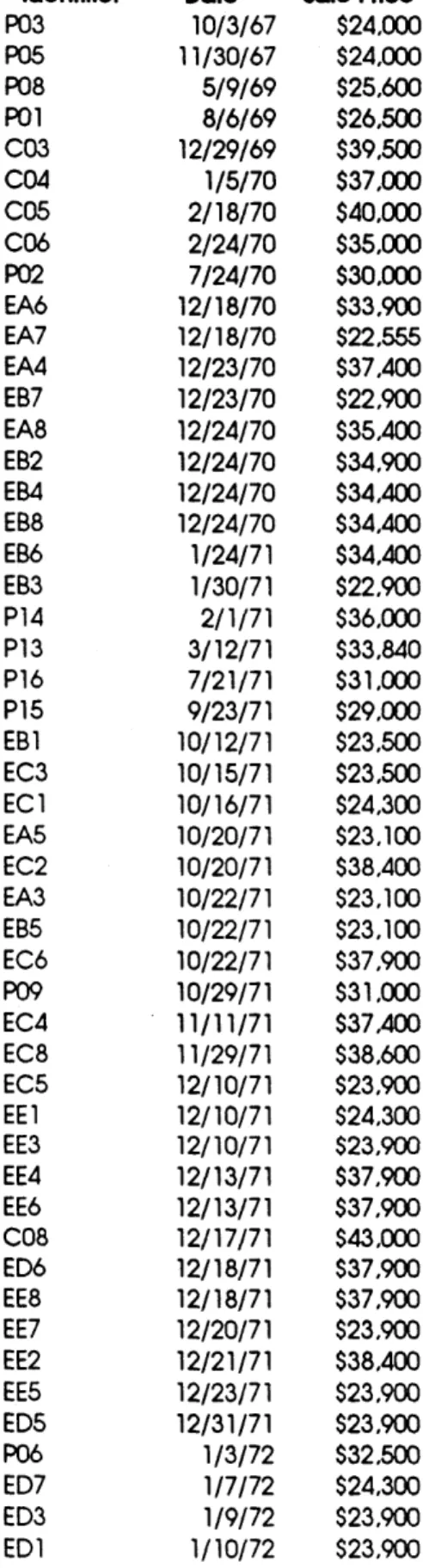
Condominium Sales

As mentioned previously, condominium sales were evaluated by studying the sales and resales of 171 condominium units in 5 different condominium projects. There were a total of 372 condominium sales over a period of 24 years (see Appendix Table A3.2 for summary of sales data). The sales data was

collected from the Vermont transfer tax receipts kept on file in the Town Clerk's office in Sherburne. The sales prices were only included for arms length

transactions in which a reasonable consideration was paid for transfer of

ownership. The sales prices are based on the value assigned to the basic real estate excluding the assigned value of personal property sold with the units. The sales prices are measured in nominal U.S. dollars.

Condominium Rents

Condominium rents for the 5 condominium projects tracked above are based on winter season weekend rates. These rents were obtained from past lodging directories kept on file by Killington Ski Resort (see Appendix Table A3.3 for a summary of condominium rental data). The lodging directories list rates for the projects as they were brought on line for rental, starting in the early seventies. There is some difficulty in tracking lodging rates over the years because the rate structure changed at various times. Some years flat rates were charged for condo units, while other years rates were a function of the occupancy. When rates were a function of occupancy, the different units in some projects had to be figured

separately because of their different sizes and potential number of occupants. An effort was made to try to compare the average annual rates for each of the units over the course of the study period. Due to a lack of sufficient data for the first couple of years in the early seventies, condo rental rates for this time frame were artificially set against the hotel rates for those years. It should be noted that this data is simply a measure of what was charged and does not reflect the occupancy rate of the units. There is no measure of occupancy rates. Rents are measured in nominal U.S. dollars.

Hotel Rents

Hotel rates for the four hotels tracked are the daily winter season room rates over the last 25 years. This data was also obtained from the Killington

Lodging Directories. The ranges listed are for varying room sizes and for the purpose of this study, average room rates were used (see Appendix Table A3.4 for a summary of hotel room rates). These rates were easier to track than the condo rates because the rate structure has remained constant over the years. Rates are charged per room based on double occupancy and, except for The Cortina Inn, are based on a modified American meal plan. The Cortina Inn rates are based on a European meal plan. As with condo rates, the hotel rates do not measure

occupancy, presumably however, the rates are a reflection of the occupancy from one year to the next. Rates are measured in nominal U.S. dollars.

Stock of Condominiums

The annual stock of condominiums in the town of Sherburne, Vermont is shown in Appendix Table A3. 1. This data is an estimate based on the years in which condominiums were first put up for sale and a survey conducted by the Town Clerk in 1990 (see Appendix Table A3.5 for survey data) counting the total number of condominium projects and units in existence at that time. This data was used to back calculate the stock and number of completions in each year.

Number of Skier Visits

The number of skier visits is the total seasonal number of skier visits to the State of Vermont as reported by the Vermont Ski Areas Association (see Table A3.1 for data). A skier visit is classified as a day, night or partial day visit of a single skier. If a multiple day pass is sold, each day that person skis is considered a skier visit. Obtaining data about skier visits at specific resorts proved to be

impossible as this is a closely guarded trade secret. The results for the entire state are better that those for Killington and Pico, however, since they show the trend in skier visits across a spectrum of resorts. If we looked only at Killington visits and tried to compare them to sales and rental prices we may get interdependence of the

results. As it is, however, we are evaluating the trend and eliminating the singularities associated with Killington.

Regional Employment

Total non-agricultural state employment data is included for Connecticut, Massachusetts, New York and New Jersey since, as mentioned previously, it is assumed that these are the primary markets for a Vermont ski home. Vermont, New Hampshire and Maine employment figures are not included since it is

assumed people in these states would not be in the market for a ski home in

Vermont. This data is summarized in Appendix Table A3.1 and was obtained from the Employment and Earnings: States and Areas record published by the Bureau of Labor Statistics.

Total Annual Snowfall

Total seasonal snowfall is included from the National Weather Service weather observation station at Chittendon, Vermont (see Appendix Table A3.1 for data). This data was obtained from the Northeast Regional Climate Center located at Cornell University in Ithaca, New York. Chittendon is the nearest observation station to Killington, approximately 10 miles north of the ski area, and is deemed a good estimate of the natural snowfall at Killington. This does not account for man-made snow on the mountains and may not reflect the actual snowfall on the mountain, but it tracks the relative amount of snowfall in the region. Snowfall is measured in Imperial inches.

Mortgage Rates

Mortgage rates are the annual national average charged by major banks as listed in The Economic Report of the President (see Appendix Table A3.1 for a summary). The real mortgage rates listed are the nominal mortgage rates minus inflation rates for each year.

Consumer Price Index

The CPI is the annual figure as listed in The Economic Report of the

President (see Appendix Table A3.1 for a summary). The CPI is used to calculate

the inflation in each year by measuring the percent increase from one year to the next.

Analysis of Data

Annual Price Index

In order to track trends over time it was necessary to convert the

voluminous amounts of sales data into annual price indices that would measure the relative sales price from one year to the next across the full spectrum of projects and units. This was done by performing a linear regression analysis on the sales data and developing a hedonic model.13 _{By performing this regression it was} possible to develop an equation that can be used to predict the sales price of any one of the units in the five condo projects by simply inputting the units

characteristics and the price index for the year in which the sale price is wanted. By developing this equation, it is possible to derive an annual price index from a group of dissimilar projects. The data from the five different condo developments and from the different unit layouts within each development can be combined to create a relative price index.

The data included in the price index equation is as follows: Ln(Sales Price of Unit)

Square Feet of Unit # Bedrooms in Unit # Bathrooms in Unit # of Floors in Unit

Dummy variable for each year from 1970 to 1992

Dummy variable for four of the five condominium developments The sales price is tabulated as a logarithmic function in order to plot the non-linear nature of sales prices over time.

The value of the dummy variables is either 0 or 1 depending on whether the variable is false or true. The dummy variable for the years is used to develop the price index. The first year of the study, 1969, is not included as a dummy variable since it is the default value. When the regression is run it yields a regression coefficient for each dummy variable which is used to derive the price index for that year relative to 1969, which is indexed as 1.

The dummy variable for the condominium developments takes into account the unique features of each. As with the year dummy variable, the condo dummy variable has a default value as well. The default project is Edgemont (EM). The other projects are Colony Club (CC), Hemlock Ridge (HR), Pico Townhouses (PT) and Whiffletree (WT). They are located in different areas with different vistas, amenities, layouts and so on. In the case of this study, the purpose is to develop an annual price index and we don't so much care about how people value the different amenities associated with condominiums. As a result we simply use one dummy variable to account for all the unique features of each development. If one was interested in how buyers value the different amenities, a separate

regression should be run with dummy variables included for each amenity. The features square footage, # of bedrooms, # of bathrooms and # floors are included since the units within a given project may have different

configurations.

The complete regression output with statistics is included in Table A2. 1. The equation is shown in tabular format with the intercept indicated and the coefficients for each of the variables shown under the heading "X Coefficient". Analysis of this equation indicates that people value property more if it has greater square footage, more bedrooms and more bathrooms -not very surprising. What is interesting, however, is that people prefer a greater number of floors for a given

Table A2.1

Regression Output Constant Std Err of Y Est R Squared No. of Observations Degrees of Freedom X Coefficient 0.000214634 0.104761488 0.01644268 0.14689685 -0.2188155 -0.155420669 -0.078408072 -0.015478657 0.019438303 0.088444965 0.111572987 0.134073826 0.290982557 0.403892754 0.543767277 0.70724903 0.600061095 0.772225373 0.803011309 0.886096128 0.85136696 0.983962197 0.978327435 0.899822561 0.76097836 0.598835145 0.695866943 -0.357570914 -0.173345947 0.02148505 0.072937252 Std Err of Coef 7.51103E-05 0.027079425 0.042031104 0.029278125 0.064398394 0.058722127 0.062264545 0.056863024 0.065353028 0.067533781 0.063771561 0.058348352 0.058414644 0.057686441 0.065957439 0.068414854 0.08118415 0.063301179 0.062818993 0.062941367 0.061222995 0.061109747 0.070482078 0.065866933 0.081210558 0.077449166 0.073951316 0.044280578 0.028872123 0.038221332 0.031712238 9.832846223 0.11908105 0.934026635 366 334 t Statistic 2.85758741 3.868674748 0.391202676 5.017290227 -3.397840958 -2.64671389 -1.259273198 -0.272209525 0.297435387 1.309640353 1.749572777 2.297816838 4.981328963 7.001519759 8.244214526 10.33765318 7.391357701 12.19922579 12.78293819 14.07812013 13.90599983 16.10155893 13.88051349 13.66121849 9.370436243 7.731976696 9.409797915 -8.075118477 -6.003921152 0.562121973 2.299971768 Sq. Feet Bedrooms Baths # Floors D70 D71 D72 D73 D74 D75 D76 D77 D78 D79 D80 D81 D82 D83 D84 D85 D86 D87 D88 D89 D90 D91 D92 DCC DHR DPT DWT

building horizontally or vertically, he/she will get greater value by building vertically for the same square footage and number of units within a building

envelope.

Once we have this equation in terms of Ln(Sales Price), we can raise the equation to the power of the natural log, e, and determine the annual price indices. This data is shown in Table A2.2. The price index for 1969 then becomes 1 since e0 _{is 1. All the years are then indexed to 1969 in nominal terms.}

For the purpose of this study it is important to convert all these nominal price indices into real price indices that can be equally compared with one another. In order to do this, all the price indices were converted into 1992 dollars by multiplying each annual price index by the 1992 CPI and dividing by the CPI for the given year. With this real price index, we are now able to analyze the trends in price over time and try to index it to other exogenous variables. A plot of this real price index over time is shown in Figure Al .1. A look at this plot shows a peak in the early seventies (when the economy was booming) followed by a steady decline through 1977 (when the economy was experiencing a recession). The prices then began to rise again reaching a peak in 1981 as the economy peaked out. The region experienced a mild recession in 1982 with a reduction in jobs. Combined with a huge increase in condo completions, this resulted in a significant drop in

prices in 1982. Real prices continued to rise from 1982 to 1987 as the economy expanded with only a small drop in 1986. After 1987, however, real prices dropped 40% over a period of four years as the economy slipped into a long recession and the effect of the overbuilding of the 1980's sank in. Since the low in 1991, prices have risen a little, but they are still substantially lower than they were six years ago.

Table A2.2

Price Index Calculation Intercept Sq. Feet Bedrooms Baths # Floors D70 D71 D72 D73 D74 D75 D76 D77 D78 D79 D80 D81 D82 D83 D84 D85 D86 D87 D88 D89 D90 D91 D92 DCC DHR DPT DWT 9.832846 0.000215 0.104761 0.016443 0.146897 -0.21882 -0.15542 -0.07841 -0.01548 0.019438 0.088445 0.111573 0.134074 0.290983 0.403893 0.543767 0.707249 0.600061 0.772225 0.803011 0.886096 0.851367 0.983962 0.978327 0.899823 0.760978 0.598835 0.695867 -0.35757 -0.17335 0.021485 0.072937 Exp. D 0.80347 0.856055 0.924587 0.984641 1.019628 1.092474 1.118035 1.143477 1.337741 1.497643 1.722484 2.028404 1.82223 2.164578 2.232253 2.425642 2.342847 2.675034 2.660003 2.459167 2.140369 1.819998 2.005447

Indices ($) PO1 0 0 1970 1971 1972 1973 1974 1975 1976 1977 1978 1979 1980 0 1981 1982 1983 1984 1985 1986 1987 1988 1989 1990 1991 1992 OOI z o D (D0 (D C). C

x

'Ut

\

l

/\

--.

\

K

-eI

-e/

--

e

+

--

e

+

o

Annual Rent Indices

As with sales prices, it was necessary to convert the rental data from the five projects and four hotels into annual indices for the purpose of analyzing trends. In this case, however, a different approach was taken. Since data was

available for each project on a whole for each year (rates were established for all condominiums in a project), a weighted average of the rents was used to determine the relative rent movement from one year to the next. This weighted average was calculated by summing the product of the total number of units in each project times the rental rate and dividing the sum by the total number of units. A similar calculation was made for hotel rents over the time period (see Tables A2.3a&b for a summary of the calculations). For the condominium rents, the first four years data was adjusted to more accurately reflect the changes measured in the hotel market since the condo data for these years was incomplete.

As with the price indices, these indices were then converted from nominal into real 1992 dollars for the sake of comparison. The same conversion process was used as that described for prices using the CPI. A plot of the real rent index over time is shown in Figure Al. 1 on page 34. This plot shows that the condo and hotel rents follow similar trends over time, with some exceptions. Real rents generally fell from 1970 through the mid-seventies during the energy crunch and the recession of the mid-seventies. Rents then began a steady increase through the late eighties with hotel rents spiking up to a record high from 1985 to 1988. Since then rents have fallen off precipitously to around 70% of their late-eighties levels.

Table A2.3a

IColony

Club

IYear

|

# Units

|

Rent/we | 1969 1970 1971 1972 1973 1974 1975 1976 1977 1978 1979 1980 1981 1982 1983 1984 1985 1986 1987 1988 1989 1990 1991 1992 175 175 200 200 238 288 313 325 350 388 475 413 475 540 468 600 672 750 670 | Edgemont # Units

|

Rent/we| Condominium Rents Condominium Project

|Hemlock

Ridge Pico Townhouse

# Units I Rent/we

|I

80 115 123 133 143 143 158 168 180 237 313 388 346 400 400 406 368 368 526 320 284 175 175 175 175 200 238 263 288 335 380 395 435 460 480 580 660 622 622 600 # Units I Rent/we I Whiffletree # Units I Rent/we

|

160 188 213 263 300 318 455 475 475 140 150 160 163 180 193 210 237 310 380 348 490 400 406 430 490 420 410 316 Condo Rent Adjusted Index Value 130 124 128 133 80 115 149.433 154.5294 166.1176 169.9381 192.1856 218.7216 239.5567 268.7526 322.2353 392.3299 391.3711 449.2887 423.4706 443.2471 444.1882 507.2941 523.8588 486.7529 419.3647

[Colonv Club IEdaemont

Table A2.3b

Hotel Rents Hotel

|Chalet Killington|

|Red Rob Inn Cortina Inn

linn

@ Long Trail

{

# Rooms

I

Rate/day| # Rooms

I

Rate/dayl # Rooms

I

Rate/dayl # Rooms |Rate/day

Year 1969 1970 1971 1972 1973 1974 1975 1976 1977 1978 1979 1980 1981 1982 1983 1984 1985 1986 1987 1988 1989 1990 1991 1992 90 90 90 90 90 90 90 90 90 90 90 90 90 90 90 90 90 90 90 90 90 90 30 32 30 32 33 35 41 45 54 60 65 70 75 88 89 115 152 180 140 151 148 150 40 39 40 40 39 43 47 48 56 67 69 88 98 108 126 134 144 153 158 158 158 168 168 Hotel Rent Index 37.68056 36.02564 37.17521 37.84188 42.5812 44.94017 45.04701 50.1453 54.65812 63.4359 69.58547 79.11966 86.51709 93.91453 101.2051 100.2051 114.2521 132.1667 154.3504 142.2906 146.5214 142.2692 140.453 38 41 42 45 58 60 56 64 64 70 75 84 97 110 90 75 86 98 116 120 120 120 120 36 39 39 42 46 50 49 52 60 70 80 92 96 100 120 125 125 123 150 160 160 141 130

Skier Visit Regression Analysis

An analysis of the ski resort real estate market has to start with an analysis of the skier market. It is intuitive that the more people there are skiing, the more people will want to rent condos or hotel rooms, or buy real estate. The more people there are renting, the higher the rents will be. The more people there are buying, the higher prices will be. Therefore, one of the factors driving rents and prices is skier visits.

Numerous regressions were run for the skier visits equation, considering factors such as the total employment in the four study states, the annual change in total

employment, the employment figures for each state separately and the seasonal snowfall figures for the area. The best regression fit was found to include a lagged combination of total regional employment and snowfall, with skier visits a function of the employment in the current year, employment in the prior year, employment two years prior and the snowfall in the current year.

The complete regression statistics for this equation are shown in Table A2.4. The equation is shown in tabular format with the intercept and variable coefficients listed. The R square of 0.893 indicates a very good correlation between the equation and the actual

results, which can be seen graphically in Figure A1.2. The favorable t-statistics from the regression output also indicate that the results are statistically significant. The signs are

also as one would expect. The employment is predominantly positive, with a negative correction, and the snowfall is positive. As employment increases or snowfall increases, skier visits increase. This means that given employment projections and snowfall forecasts, the model can accurately predict the number of future skier visits.

---Table A2.4

Skier Visits Regression Statistics Multiple R R Square Adjusted R Square Standard Error Observations Analysis of Variance 0.945055084 0.893129112 0.867983021 354242.0836 22 df Sum of Squares 4 1.78281E+13 17 2.13329E+12 21 1.99613E+13 Mean Square F 4.45701E+12 35.51761192 1.25487E+11 Significance F 4.77946E-08

Coefficients Standard Error t Statistic P-value Lower 95% Upper 95%

-11813750.1 0.858473842 -0.579128925 0.657589231 19429.16566 1496499.058 0.308848207 0.557899766 0.323012655 4447.345474 -7.894258297 2.779597948 -1.038051923 2.035800212 4.368710678 1.01867E-07 0.011231301 0.311051359 0.054581502 0.000269055 -14971091.54 0.206860174 -1.756196185 -0.023908852 10046.07379 -8656408.67 1.510087511 0.597938336 1.339087314 28812.25753 Regression Residual Total Total Emp Total Emp Total Emp Snowfall Intercept x1 x2 x3 I

Skier Visits 1971 1972 1973 1974 1975 1976 1977 1978 1979 1980 fD 1981 ' 1982 1983 1984 1985 1986 1987 1988 1989 1990 1991 1992

01

Of course, however, the skier forecasts are only as good as the forecasted data put into the equation. Employment data can probably be forecast with some accuracy by economic experts given the economic indicators in a region. This data will be used in the later chapter on forecasting. The real problem with this equation, however, is the

importance of snowfall and the lack of a reliable means of predicting seasonal snowfall in a region. One could look at the Farmer's Almanac to get a sense of how much snowfall might occur in a given year, but this is still very much a shot in the dark. It is very difficult to predict with any accuracy what the snowfall several years in the future will be since it is very much a function of climatological weather patterns which are constantly changing.

It is significant to note that skier visits are very well correlated with snowfall. Of all the factors considered, the t-statistic for snowfall is the highest, 4.37, however, the significance of the variable has been diminishing over the last decade. A plot of the variables over time shows this trend. Figure A1.3 tracks the skier visits, snowfall, and employment figures over the last 23 years. This figure yields some interesting results. Up until the early eighties, skier visits in a given year closely followed the amount of natural snowfall in that year, with peaks in 1971, 1978 and 1982, and troughs in 1974 and 1980. After 1982, however, the relationship of visits and snowfall begins to separate with snowfall trending downward and visits trending upward. This phenomenon is probably the result of the introduction of snowmaking equipment at most Eastern ski areas. Up until the early 1980's most areas relied upon natural snow and hence rode the weather roller coaster from one year to the next. With the advent of modern snowmaking, ski areas have been able to smooth the skier visit cycle somewhat.

The other interesting result is that prior to the early 1980's there was a smaller relationship between skier visits and employment, in fact there was a reverse lag during the

1970's where employment followed skier visits by about one year. Whether this is coincidence or not is unknown. Then starting in the early 1980's, the employment seems to become more of a determining factor in predicting skier visits. The employment in the

Skier Visits II I I 1970 1971 1972 1973 1974 1975

1976

1977 1978 1979 1980 + * 1981 1982 1983

/

1984 1985

T

1986 1987 1988 1989 1990. 1 I I I I || Employment

I

|

T

0 D D 94

current year seems to be the primary factor with the employment one and two years back contributing to the equation. This may be the result of the increasing cost of skiing. Over the last decade the cost of skiing has skyrocketed as equipment and lift expenses have

continued to increase. As a result of the increased cost, skier visits have become more dependent upon employment.

Another factor which may affect skier visits and has been neglected from the study is the effect of advertising and how the skier market has responded to it. How many people ski and how has the number changed over the years? This data was not readily available for study, but it seems that the popularity of the sport has substantially increased over the years and is to some extent a function of demographic patterns. The skier market is predominantly younger, affluent people aged 18 to 35 with incomes between $25,000 and $50,000.14 Over the last five years, there has a been a slowdown in the growth of the skier market. In explaining this, Logan and Day say:

"A number of factors are responsible for this slowdown: fewer and shorter visits by habitual skiers; a decline in leisure time; more competing choices for that leisure time; a slow growth in the population of new skiers; and the aging of the population... .The slowdown of growth in skier days is largely

a matter of changing demographic patterns. The aging of the baby boomers is taking its toll on the skier market...Although participation rates among the older population are projected to improve over the next

few years, this improvement will not offset the loss in the number of skiers under 35."15

Figure A1.3 on page 42 shows this considerable decline in skier visits over the last several years from a peak in 1987.

In either event, there appears to be a strong correlation between employment and skier visits as well as a diminishing yet still important correlation between natural snowfall and skier visits. As time progresses and demographics change, it will be important to

14Logan and Day, "Ski Resort Real Estate Development", p. 37. 15_{Logan and Day, "Ski Resort Real Estate Development", pp. 37-38.}

update this model to account for the changing demographic patterns. For the time being, however, the model provides a good estimate of skier visits and will be used to forecast