Distributed parameter estimation for complex energy systems

Distributed Parameter Estimation for Complex

Energy Systems

by

Janak Agrawal

B.S. Electrical Engineering and Computer Science

Massachusetts Institute of Technology, 2019

Submitted to the Department of Electrical Engineering and Computer

Science

in partial fulfillment of the requirements for the degree of

Master of Engineering in Electrical Engineering and Computer Science

at the

MASSACHUSETTS INSTITUTE OF TECHNOLOGY

September 2020

c

○ Massachusetts Institute of Technology 2020. All rights reserved.

Author . . . .

Department of Electrical Engineering and Computer Science

August 10, 2020

Certified by . . . .

Marija Ilic

Senior Research Scientist

Thesis Supervisor

Accepted by . . . .

Katrina LaCurts

Chair, Master of Engineering Thesis Committee

Distributed Parameter Estimation for Complex Energy

Systems

by

Janak Agrawal

B.S. Electrical Engineering and Computer Science

Massachusetts Institute of Technology, 2019

Submitted to the Department of Electrical Engineering and Computer Science on August 10, 2020, in partial fulfillment of the

requirements for the degree of

Master of Engineering in Electrical Engineering and Computer Science

Abstract

With multiple energy sources, diverse energy demands, and heterogeneous socioe-conomic factors, energy systems are becoming increasingly complex. Multifaceted components have non-linear dynamics and are interacting with each other as well as the environment. In this thesis, we model components in terms of their own internal dynamics and output variables at the interfaces with the neighboring components.

We then propose to use a distributed estimation method for obtaining the pa-rameters of the the component’s internal model based on the measurements at its interfaces. We check whether theoretical conditions for distributed estimation ap-proach are met and validate the results obtained. The estimated parameters of the system can then be used for advanced control purposes in the HVAC system.

We also use the measurements at the terminals to model and verify the compo-nents in the energy-space which is a novel approach proposed by our group. The energy space approach reflects conservation of power and rate of change of reactive power. Both power and rate of change of generalized reactive power are obtained from measurements at the input and output ports of the components by measuring flows and efforts associated with their ports. A pair of flow and efforts is measured for electrical and gas ports, as well as for fluids. We show that the energy space model agrees with the conventional state space model with a high accuracy and that standard measurements available in a commercial HVAC can be used for calculating the interaction variables in the energy space model.

A novel finding is that unless measurements of both flow and effort variables is used, the sub-model representing rate of change of reactive power can not be validated. This implies that commonly used models in engineering which assume constant effort variables may not be sufficiently accurate to support most efficient control of complex interconnected systems comprising multiple energy conversion processes.

Thesis Supervisor: Marija Ilic Title: Senior Research Scientist

Acknowledgments

I would first like to express my utmost gratitude to my supervisor Prof. Ilic without whose support this thesis would not have come to fruition. Her guidance and constant feedback has been essential throughout my Masters in keeping me motivated and producing a high quality of work.

I would also like to thank my group at LIDS at MIT and it has been a great learning experience working with my co-researchers. I would like to thank Pallavi Bharadwaj for the encouragement and valuable input in my work. I am also grateful to Dan Wu, Anna Jevtic and Rupamathi Jaddivada whose previous work has been essential for this thesis. The immense progress that we have made in this project is a result of the productive collaboration and efficient team work amongst our group. Thank you for the constant support and fun conversations.

I also appreciate all the help received from Mike Gao, Min Zhang, Le Li, Jinyi Zhang and others at ENN Science and Technology Development. Thank you for sponsoring my Masters as a part of Dynamic Monitoring and Decision Systems (Dy-MonDS) Framework for IT-enabled Engineering of Retail-level Energy Services (RES) project (MIT Reference: 6940611). This wouldn’t have been possible without your help and collaboration. I am grateful for your hard work and thoughtfulness in pro-viding us with the information we needed.

Last but not the least, I would like to thank MIT CSAIL and MIT Energy Initia-tive for giving me this opportunity and all the administrators/staff who helped me stay on track during my Masters.

Contents

1 Introduction 15

1.1 Motivation . . . 15

1.2 State of the Art . . . 16

1.3 Contribution . . . 17

1.4 Outline . . . 18

1.5 List of Publications . . . 19

2 Background 21 2.1 Description of HVAC system . . . 21

2.1.1 Components of HVAC . . . 21

2.1.2 Thermal Subsystem . . . 24

2.1.3 Water Flow Subsystem . . . 26

2.1.4 Air Flow Subsystem . . . 26

2.2 Gray Box System Identification . . . 26

2.2.1 Non-linear least squares . . . 27

2.2.2 Gauss-Newton Method . . . 28

2.3 Decomposition of Interconnected System . . . 29

2.3.1 Diagonally Dominant Matrices . . . 29

2.3.2 Dynamics of Interconnected Systems . . . 30

2.4 Energy-Power state space modelling . . . 31

2.4.1 Pitfalls of Conventional Modelling . . . 31

2.4.2 Novel Energy-Power Modelling Methodology . . . 33

3 Approach 37

3.1 Overview . . . 37

3.2 Energy Consumption inside the HVAC . . . 38

3.2.1 Electricity consumption in HVAC . . . 38

3.2.2 Gas consumption in the HVAC . . . 40

3.3 Modelling of HVAC components in Conventional state space . . . 43

3.3.1 Electric Chiller Model . . . 43

3.3.2 Water Pump Model . . . 44

3.3.3 Chiller and Pump combined model . . . 47

3.4 Decoupling of Chiller and Pump subsystem . . . 48

3.4.1 Assumptions . . . 48

3.4.2 Coupling between Pump and Chiller . . . 52

3.5 Distributed Parameter Estimation . . . 54

3.6 Energy Space model for chiller . . . 55

4 Implementation 59 4.1 Data Description . . . 59

4.2 System Identification in MATLAB . . . 60

4.3 Energy space model verification in Python . . . 62

5 Results 65 5.1 Distributed Parameter Estimation . . . 65

5.1.1 Chiller Subsystem Identification . . . 65

5.1.2 Pump Subsystem Identification . . . 67

5.2 Energy Space Model Verification . . . 69

5.2.1 First Fundamental equation verification . . . 70

5.2.2 Second Fundamental Equation Verification . . . 72

5.2.3 Effects of Pressure . . . 73

6 Conclusion 77 6.1 Conclusion . . . 77

List of Figures

2-1 Decomposition of the full interconnected HVAC system into air flow,water

flow and thermal subsystems . . . 22

2-2 Multi-Energy flow model of commercial HVAC System [14] . . . 23

2-3 Multi-Energy flow model of commercial HVAC System . . . 25

2-4 Schematic of a HVAC system in open loop (borrowed from [25]) . . . 32

2-5 Stand-alone component in open-loop in energy space (borrowed from [23]) . . . 34

3-1 Electricity consumption of Electric Chillers . . . 39

3-2 Electricity consumption of Water Pumps . . . 39

3-3 Total Electricity Consumption of HVAC . . . 40

3-4 Gas consumption and electricity production of ICG . . . 41

3-5 Gas consumption of Chiller and Boiler . . . 42

3-6 Gas consumption and cooling demand of HVAC . . . 42

3-7 Interaction of pump and chiller subsystem with the HVAC [33] . . . 47

3-8 Chiller control vs Temperature difference across chiller [33] . . . 50

3-9 Pump control in response to supplied water temperature [33] . . . 51

3-10 Interface varibales for the HVAC system [14] . . . 55

3-11 Chiller models in conventional and energy state space . . . 56

4-1 Chiller MATLAB Model file . . . 60

4-2 Chiller grey box model in MATLAB . . . 61

4-3 Chiller grey box model optimization in MATLAB . . . 61

4-5 Using Numpy to convert units of data . . . 62

4-6 Using Numpy calculate rate of reactive power flow in Chiller . . . 63

4-7 Differentiation and Integration in Python . . . 63

5-1 Chiller Model Parameter Estimation [33] . . . 66

5-2 Pump model Parameter Estimation [33] . . . 68

5-3 Available Chiller Measurements [14] . . . 69

5-4 Calculation of stored energy in chiller [14] . . . 71

5-5 Calculation of energy in tangent space for chiller [14] . . . 73

5-6 Pressure difference across chiller [14] . . . 74

5-7 Calculation of energy in tangent space for chiller without contribution of pressure [14] . . . 75 5-8 Correlation between ˙𝑄 and rate of change of pressure across chiller [14] 75

List of Tables

3.1 Analogous effort and flow variables across different energy domains [24] 56 4.1 Summary of measurement data from the HVAC . . . 59 5.1 Estimated Chiller Subsystem Parameters [33] . . . 65 5.2 Estimated Pump Subsystem Parameters [33] . . . 67

Chapter 1

Introduction

1.1

Motivation

With the growing demand of energy worldwide, there is a real urgency for developing more intelligent energy systems, especially ones that can be implemented today. With multiple energy sources and diverse energy demands, energy systems are becoming increasingly complex and multifaceted. For example, in this thesis we consider a complex heating-ventilation-air conditioning (HVAC) systems which consists of sev-eral components with non-linear dynamics including water, gas, electricity and air networks interacting with each other as well as the environment. Therefore, it is becoming challenging to improve the efficiency of such complex systems without im-proving upon the existing techniques used for mapping and controlling these systems. To address these challenges, we propose a novel approach to mapping and monitoring integrated energy systems.

HVAC’s are extensively used in household as well as commercial building and account for 30% of the total electricity consumption in buildings in US [19]. The ma-jority of HVAC controllers still operate on old-age classical methodologies which are often based on pre-programmed logic [36]. However, more advanced control strate-gies like model predictive control (MPC) [10] [26] or adaptive control [27] [37], which are harder to implement, can more efficiently track the heating/cooling load of the building, thus, reducing the overall energy consumption of a building [11] [12]. These

advanced strategies require basic knowledge of system model, which is generally com-plex, interconnected and has unknown parameters. Therefore, we need an estimator which is responsible for calculating the unknown parameters of the system using prior knowledge as well as real-time measurements. The output of the estimator is given to the control and the accuracy of the control is directly dependent on the accuracy of the estimator. To further improve state-of-the-art system control algorithms we need to advance state estimation of complex systems.

This thesis also concerns with the difficult problem of managing complex inter-connected dynamical systems. With the growing energy demand, energy systems in the future will be more complex comprising heterogeneous sub-components involving multi-energy conversions. Overcoming the complexity of modelling these systems is essential for efficient energy-conversion control. Therefore, we utilize a novel modeling to derive an aggregate, low-order, dynamical model of these components [22] [25].

1.2

State of the Art

Designing efficient control for a complex system requires knowledge about the em-pirical parameters of the components of the system. Traditionally these emem-pirical parameters have been estimated by employing expensive sensors such as mass flow meters. But use of mass flow meters in every case is not possible which may lead to a badly tuned model. To avoid this problem, modern controllers rely on experimental mappings between the desired outputs, and the power consumed by the controllers, much the same way as in frequency regulation one relies on generator droops [29] [21]. Their performance depends on the internal dynamics of equipment and their feedback control. The main challenge is how to increase efficiency without requiring complex fast fail-prone communications while having only limited measurements for control.

This problem is even more tangible in large interconnected systems. While the structure of these large interconnected systems is extensively studied, the question concerning the decomposition of the interconnected system while taking into account

the availability of measurements and control is rarely studied. In this thesis we take a general large-scale dynamical systems point of view and recall conditions under which a complex system can be decomposed into subsystems whose local measurements are sufficient for distributed parameter estimation. We use real world measurement data to show that such a decomposition works well for the HVAC system under consideration and can be key to determining unknown parameters of large dynamical energy systems. To the best of our knowledge, this question has not been addressed in the previous literature of large-scale dynamical systems.

From the systems perspective, traditionally power grids have been studied by utilizing Thevenin and Norton’s equivalent circuits recomputed every timestep, the accuracy of which depends on the chosen interaction protocols and are generally not scalable to very large systems. This has been a valid approach in the past when the disturbances entering the grid such as those from the renewables and did not form a high fraction of the generation portfolio. Typically, the benchmark problems for the energy management are non-convex. To apply any decomposition strategy, these constraints are all simplified by applying convex approximations. These approaches, however, are not scalable [22] [25]. Here, we verify a novel energy-power modelling approach which uses effort and flow variables at interfaces to design aggregate models of complex systems in multi-energy domains. We use this approach to show that it can be easily applied to a commercial HVAC system and hence be used to account for the complexity of a commercial HVAC system and can help design controllers which can respond to fast-response disturbances which are often ignored in conventional state space controllers.

1.3

Contribution

The main objective of this thesis has been to perform distributed parameter estima-tion in complex dynamical systems using only available measurements.

Majority of literature regarding parameter estimation for power systems has been focused on a single component fixed to a test bench. In this thesis, we tackle the issue

of distributed parameter estimation for an interconnected system using measurement data from a real world HVAC system.

The energy-power space was introduced for modeling interactions in multi-energy systems using aggregate interaction variables. It was shown that real power and generalized reactive power can be defined for any type of energy system by using analogies for efforts and flows. They represent interaction variables whose dynamical models are sufficient to model input-output characteristics of components and their interactions within the complex system. This modelling was originally derived for electrical systems and has been proved for several electrical devices [23] [22]. In this thesis, for the first time, we verify the energy-power space model of an industrial chiller using sensor measurement. Such an approach has never been used before to model a component in a commercial HVAC.

This thesis addresses some of the most prominent issues regarding models and their parameters still challenging the design of efficient controls for HVACs. In this thesis we use an HVAC system to verify our methodology but its versatility in being applicable to a huge array of systems opens up a lot of possibilities for future smart controllers.

1.4

Outline

The remainder of the thesis is outlined as follows:

Chapter 2 provides an overview and component level description of the HVAC system under consideration. We also provide a brief background on the work that this paper builds upon.

Chapter 3 discusses previous work done in this field of research and their effec-tiveness.

Chapter 4 describes the approach used to model the components and estimate unknown parameters in the HVAC system.

Chapter 5 describes the tools used to implement the approach in Chapter 4. Chapter 6 states the numerical results obtained using the methodology specified

in Chapter 4.

Chapter 7 concludes with the contributions of this thesis and future work.

1.5

List of Publications

These publications formulated during the Masters project are the core of this thesis:

1. P. Bharadwaj, J. Agrawal, R. Jaddivada, M. Zhang and M. Ilic. Measurement-based Validation of Energy-Space Modelling in Multi-Energy Systems.

Submitted to 2020 North American Power Symposium (NAPS).

2. D. Wu, J. Agrawal, P. Bharadwaj, L. Li, J. Zhang and M. Ilic. On The Validity of Decomposition for Distributed Parameter Estimation in Complex Dynamical Systems: The Case of Cooling Systems.

Chapter 2

Background

2.1

Description of HVAC system

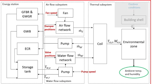
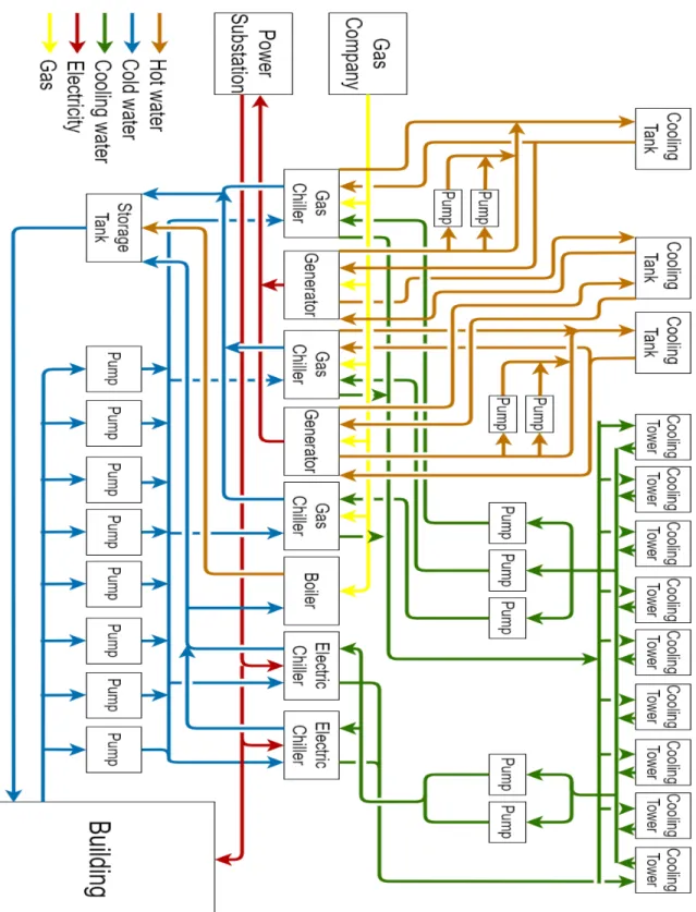
For this thesis, we have used data from a real-world HVAC system that offers heating, cooling and power to a commercial building over the year. The HVAC system consists of electricity, gas, airflow and waterflow networks as its main components which can also be seen in Fig. 2-1. A more detailed sketch of the same HVAC system can be seen in Fig. 2-3. We can see the flow of different forms of energy such as gas and electricity in these figures and how the various networks interact with each other.

This is a complex HVAC system with a cooling capacity of 500 MW, heating capacity of 500MW and power generation capacity of 40 MW. Here we provide a brief description of all the components that are present in this HVAC system and also analyse the flow of energy from one component to another.

2.1.1

Components of HVAC

Although, the HVAC contains several components, small and big, which are essential for its functioning, here we focus on a few major components of the HVAC which consume the most energy and are also studied upon in the rest of the thesis. A detailed sketch of all the components can be found in Fig. 2-3, whereas, a simplified sketch of the components showing the measurements and control law of the components can

Figure 2-1: Decomposition of the full interconnected HVAC system into air flow,water flow and thermal subsystems

be found in 2-2.

Electric Chiller

An electric chiller, or more commonly known as centrifugal chiller, utilizes the vapor compression cycle to chill water and reject the heat collected from the chilled water plus the heat from the compressor to a second water loop cooled by a cooling tower [32]. We can see the sketch of the electric chiller in Fig. 2-2 (a).

Gas Chiller

A gas chiller also known as an absorption chiller consists of a evaporator, absorber, generator and heat exchanger. The chilled water is cooled down using a sudden change of pressure. First, the water is heated up in the generator which releases the water from the refrigerant and becomes vapor. Then, the vapor is transported to the evaporator where the low pressure cools down the water. Gas chillers can use different refrigerants like Li-Br or NH3-water. Since, they can operated using natural

(a) Electric Chiller (b) Gas Chiller

(c) Water pumps (d) Storage Tank

(e) Gas Boiler

(f) Air Handling Unit (AHU)

Figure 2-2: Multi-Energy flow model of commercial HVAC System [14]

gas or flue gases from other components, they are increasingly becoming common in commercial HVAC [15]. A diagram can be seen in Fig. 2-2 (b).

Water pumps

The water pumps used in this HVAC are centrifugal pumps which are placed along the water pipelines. There are two big arrays of water pumps, one for the water input of chillers and boilers, and other for the water input to the air-conditioning coils which can be seen in Fig. 2-3.

Storage Tank

A storage tank takes in the hot or cold water incoming from the chillers or boilers respectively and stores it until it needs to be transported to the air handling units.

Gas Boiler

The gas boiler burns natural gas and heats up the water supplied to it using the pumps. The output water is then stored in the storage tank.

Air Handling Unit

A commercial air handling unit or AHU consists of a fan, an electric purifier and a coil for hot/cool water. They take fresh ambient air from outside, clean it, heat or cool it and then transport it to a designated area of a building using ducts [9].

2.1.2

Thermal Subsystem

The thermal subsystem mainly consists of the coil (i.e. heat ex-changer), chillers, boilers, internal combustion generator (ICG) and thermal zones within the building shell.

In summers, the water is chilled to the desired temperature using the chillers and stored in a storage tank until delivered to the air-conditioning coils. The waste heat is discarded to the environment with the use of cooling towers shown in Fig. 2-3. In winters, the boiler and waste heat from ICG is used to heat up the water and pumped to the coil. The chillers and boilers are powered using electricity and gas bought from

the state power grid and third-party company respectively. We provide a detailed analysis of energy consumption in thermal subsystem in Section 3.

2.1.3

Water Flow Subsystem

The waterflow subsystem is mainly comprised of the chillers, boilers, ICG, water pipeline network, water pumps, storage tank and the coil inside the air handling units (AHU).

Fresh and clean water is supplied by a third-party company which is then delivered to the chillers or boiler using the water pumps. Water is cooled or heated according to demand and is stored in the storage tank and delivered to AHUs using water pumps and a pipeline network as per demand.

2.1.4

Air Flow Subsystem

The air flow system consists of the AHUs inside the buildings and the coils.

The AHU takes in ambient air from outside and the temperature-controlled water inside the coils exchanges heat with the air and then, the cooled/heated air is then delivered to the respective thermal zone using ducts.

2.2

Gray Box System Identification

This section presents an approach at identifying system parameters of the HVAC using sensor measurements. For this purpose, many combinations and nuances of theoretical modeling from first principles and empirical modeling based on measurement data can be pursued. Basically, the following three different modeling approaches can be distinguished [28]:

1. White box models are those which can be derived directly from first principles and all parameters can be determined by theoretical modeling.

2. Black box models requires both model structure and parameters to be deter-mined from experimental modeling.

3. Gray box models represent a compromise or combination between white and black box models. They are characterized by an integration of various kinds of infor-mation that are easily available.

Rarely we find pure white box or black box approaches in reality. Often the model structure may be determined by first principles but the model parameters may be estimated from data [20]. We use a similar approach in our analysis here and thus make use of gray box system identification techniques.

2.2.1

Non-linear least squares

Since we have no prior knowledge about the distribution of the parameters as well as the noise in the data, we assume that parameters are uniformly distributed over a given range and the noise is white with constant variance. Such a system can be efficiently identified using Non-Linear Least squares and optimized using Newtons method [28] [20].

For non-linear optimization algorithms, quadratic loss function is by far the most common in practice. If the parameters are linear, a least squares problem originates but for non-linear parameters, the loss 𝐸(𝜃) becomes,

𝐸(𝜃) = 𝑁 ∑︁ 𝑖=1 𝑓2(𝑖, 𝜃) (2.1) = 𝑓𝑇𝑓 𝑤ℎ𝑒𝑟𝑒, 𝑓 = [𝑓 (1, 𝜃) ... 𝑓 (𝑁, 𝜃)]𝑇 (2.2)

and is known as non-linear least squares problem. Let the modified Jacobian be,

𝐽′ = ⎡ ⎢ ⎢ ⎢ ⎣ 𝛿𝑓 (1, 𝜃)/𝛿𝜃1 ... 𝛿𝑓 (1, 𝜃)/𝛿𝜃𝑁 : : 𝛿𝑓 (𝑁, 𝜃)/𝛿𝜃1 ... 𝛿𝑓 (𝑁, 𝜃)/𝛿𝜃𝑁 ⎤ ⎥ ⎥ ⎥ ⎦ (2.3)

The jth component of gradient of this loss function can be written as 𝑔𝑗 = 𝛿𝐸(𝜃) 𝛿𝜃𝑗 = 2 𝑁 ∑︁ 𝑖=1 𝑓 (𝑖, 𝜃)𝛿𝑓 (𝑖, 𝜃) 𝛿𝜃𝑗 (2.4)

Therefore, the gradient can be written as,

𝑔 = 2𝐽𝑇𝑓 (2.5)

2.2.2

Gauss-Newton Method

The Gauss-Newton method is the non-linear least squares version of the general New-tons method [28].

the goal of optimization is that each iteration step should decrease the loss function value, i.e., 𝐸(𝜃𝑘) < 𝐸(𝜃𝑘−1). For a general gradient-based optimization, the principle

is to change the parameter vector 𝜃 proportional to some step size 𝜂𝑘−1 into a direction

𝑝𝑘−1:

𝜃𝑘 = 𝜃𝑘−1− 𝜂𝑘−1* 𝑝𝑘−1 (2.6)

The vector 𝑝𝑘 for Newtons method is given by,

𝑝𝑘 = 𝐻_𝑘−1−1 * 𝑔𝑘−1 (2.7)

which is the gradient of the error rotated by multiplying with the Hessian of the loss function. Hence, for Newton’s method all second order derivatives of the loss function have to be known analytically or estimated by finite difference techniques.

Gauss-Newton method assumes a small residual error in the loss function and thus approximates the Hessian as 𝐽𝑇_{𝐽 . Therefore, the Gauss-Newton Algorithm becomes,}

𝜃𝑘 = 𝜃𝑘−1− 𝜂𝑘−1* (𝐽𝑇𝐽 )−1* 𝑔𝑘−1 (2.8)

It approximately shares the properties of the general Newtons method but does not require a second order derivative to be calculated.

2.3

Decomposition of Interconnected System

This section provides an introduction to the generalized theory of diagonally dominant matrices and how diagonally dominant matrices can be used to reduce the complexity of an interconnected system.

2.3.1

Diagonally Dominant Matrices

Let A be any arbitrary square matrix with complex entries, which is partitioned in the following manner:

𝐴 = ⎡ ⎢ ⎢ ⎢ ⎢ ⎢ ⎢ ⎣ 𝐴1,1 𝐴1,2 ... 𝐴1,𝑁 𝐴2,1 𝐴2,2 ... 𝐴2,𝑁 : : 𝐴𝑁,1 𝐴𝑁,2 ... 𝐴𝑁,𝑁 ⎤ ⎥ ⎥ ⎥ ⎥ ⎥ ⎥ ⎦ (2.9)

where, the diagonal submatrices 𝐴𝑖,𝑖 are square of order 𝑛𝑖.

If the diagonal submatrices 𝐴𝑗,𝑗 are non-singular and if

(||𝐴−1_𝑗,𝑗||)−1 ≥ 𝑁 ∑︁ 𝑘=1,𝑘̸=𝑗 ||𝐴𝑗,𝑘|| (2.10) 𝑓 𝑜𝑟 𝑎𝑙𝑙 1 ≤ 𝑗 ≤ 𝑁

then A is block diagonally dominant relative to partitioning 2.9. We can define (||𝐴−1_𝑗,𝑗||)−1 _{to be zero whenever 𝐴}

𝑗,𝑗 is singular.

In the special case that all the submatrices 𝐴𝑖,𝑗 are 1 × 1 matrices, then equation

|𝐴𝑗,𝑗| ≥ 𝑁 ∑︁ 𝑘=1,𝑘̸=𝑗 |𝐴𝑗,𝑘| (2.11) 𝑓 𝑜𝑟 𝑎𝑙𝑙 1 ≤ 𝑗 ≤ 𝑁

which is the general definition of diagonal dominance of a matrix [17] [13]. If strict inequality holds, then we say that the matrix is strictly diagonally dominant.

2.3.2

Dynamics of Interconnected Systems

We can write the conventional state space model of a large interconnected dynamical system as follows [31]: ˙𝑥𝑖 = ˜𝐴𝑖𝑖𝑥𝑖+ ∑︁ 𝑗̸=𝑖 ˜ 𝐴𝑖𝑗𝑥𝑗+ ˜𝐵𝑖𝑢𝑖 (2.12)

where 𝑗 ∈ 𝐶𝑖 is set of connections to the subsystem 𝑖.

For network interconnected system, equation 2.12 can be re-written as

˙𝑥𝑖 = 𝐴𝑖𝑖𝑥𝑖+

∑︁

𝑗̸=𝑖

𝑅𝑖𝑗𝑦𝑗 + 𝐵𝑖𝑢𝑖 (2.13)

where 𝑦𝑗 are output variables measured at the interconnection of subsystem 𝑖 and

𝑗 ∈ 𝐶𝑖.

We need to first derive the conditions for decomposition of the interconnected system and then implement distributed parameter estimation for the model. Us-ing the general Metzler conditions, we use the more restrictive but simpler diagonal dominance as sufficient conditions for decomposition [30] [18].

Using the definition given in equation 2.11, we can say that an uncontrolled in-terconnected dynamical system is diagonally dominant if the system matrix satisfies

|𝐴𝑖𝑖,𝑘𝑘| ≥ ∑︁ 𝑗̸=𝑖 ∑︁ 𝑟̸=𝑘 |𝑅𝑖𝑗,𝑘𝑟| + ∑︁ 𝑟̸=𝑘 |𝐴𝑖𝑖,𝑘𝑟| (2.14)

where 𝐴𝑖𝑖,𝑘𝑘 is the 𝑘-th diagonal element of subsystem-𝑖; 𝑅𝑖𝑗,𝑘𝑟 is the 𝑟-th element

of row-𝑘 of the interface between subsystem-𝑖 and subsystem-𝑗; 𝐴𝑖𝑖,𝑘𝑟 is the 𝑟-th

element of row-𝑘 of subsystem-𝑖.

Gershgorin Circle Theorem states that if a matrix is strictly diagonally dominant with all diagonal entries being negative, the real parts of its eigenvalues are also negative which suffices stability at equilibrium [17].

2.4

Energy-Power state space modelling

Conventional modelling of systems and control algorithms such as Automatic Gener-ation Control (AGC) often suffer from a lack of scalability and cannot respond to fast persistent disturbances in the system . The system might also contain several smaller devices whose physical models are not always available. This problem has been a focus of our group who have been working on a novel aggregate modeling approach that utilizes energy/power space dynamics. This modelling approach addresses the fundamental issues of limited sensor measurements and still supports fast control im-plementation [22] [24]. This model relates the rate of change of work done and rate of change of work wasted because of the the interactions with the environment.

2.4.1

Pitfalls of Conventional Modelling

There has been extensive work and very detailed models designed for HVAC control, but upto our knowledge none of these controllers view an HVAC as a complex dy-namical system whose efficiency can be enhanced by optimizing interactions between its different components. To do so, it is necessary to model different components to the degree of detail obtainable using available measurements [25].

Figure 2-4: Schematic of a HVAC system in open loop (borrowed from [25])

an RC model of the thermal zone to be heated/cooled. We denote the state variables of the space using a vector 𝑥𝑇 which represents the temperatures of various zones.

These spaces are usually cooled using air blown from an Air Handling Unit or AHU. Let us denote the state variables of the AHU as 𝑥𝑎 with states corresponding to the

fan and motor in the AHU as 𝑥𝑓 and 𝑥𝑚 respectivly. Therefore, we can represent the

dynamic model of the system as

˙𝑥𝑇 = 𝑓𝑇(𝑥𝑇, 𝑥𝑎) (2.15)

˙𝑥𝑎 = 𝑓𝑎(𝑥𝑎, 𝑢) (2.16)

An open-loop schematic for the same system is shown in Fig. 2-4. Here, depending on the choice of granularity required, the number of state variables in the model can grow extremely large. Also the exact models for the AHU and thermal zone are also complex [25]. Finally, obtaining the parameters of the model of the zone, 𝑓𝑇 can be

difficult making the model less accurate. We thus propose a simpler approach that uses aggregate energy variations in the next section.

2.4.2

Novel Energy-Power Modelling Methodology

The dynamical model of each component of a general system can be expressed in a standard state-space form as

˙𝑥𝑖 = 𝑓𝑥,𝑖′ (𝑥𝑖, 𝑢𝑖, 𝑚𝑖, 𝑟𝑖) (2.17)

𝑦𝑖 = 𝑓𝑦,𝑖′ (𝑥𝑖, 𝑢𝑖, 𝑚𝑖, 𝑟𝑖) (2.18)

𝑥𝑖(0) = 𝑥𝑖,0 (2.19)

where 𝑥𝑖, 𝑢𝑖, 𝑚𝑖, 𝑟𝑖 and 𝑦𝑖 denote local states, inputs, local disturbances, port

inputs and local outputs of interest respectively. A subset of the variables appear at the ports which can classified as either flow-type or effort-type. At the ports, one of these pairs is local to the component whereas the other is dictated by its connection to the rest of the system also called a port input.

It has been shown in [23], that using the state variable, and effort and flow variables at the port we can obtain the instantaneous real 𝑃𝑖 and reactive power ˙𝑄𝑖 appearing

at any of the ports as well as the stored energy 𝐸𝑖 and stored energy in tangent space

𝐸𝑡,𝑖.

We define a simple model that captures the dynamics of energy exchanges of a component with its neighbours by modelling the dynamics of aggregate variables, energy 𝐸 and its rate of change as follows:

˙

𝐸 = 𝑃 − 𝐸

𝜏 = 𝑝 (2.20)

˙

𝑝 = 4𝐸𝑡− ˙𝑄 (2.21)

Here, the first equation denotes the first law of thermodynamics and states that the rate of change of stored energy is directly proportional to the power input minus the dissipative losses. The second equation corresponds to the second law of ther-modynamics and highlights the inefficiencies in the system. This model was derived for general electrical circuits and was proven to hold for complex electro-mechanical systems with multi-energy conversions with the help of effort-flow analogy in different

domains [22] [25].

The dynamics of interaction variables [𝐸𝑖, 𝑝𝑖] captures the dynamics of internal

energy conversion processes without the need to specify the type of energy conversion. Although, the variables [𝐸𝑖, 𝑝𝑖] are specific to a component, they are driven by the

interactions from rest of the system through real and reactive power inputs.

Figure 2-5: Stand-alone component in open-loop in energy space (borrowed from [23])

An example of a stand-alone component in open-loop in energy space can be seen in Fig. 2-5. The bottom layer with the detailed dynamics in conventional space is utilized for designing control in energy-power space and the top layer characterizes the input-output interactions of the component.

The model was originally derived for general electrical circuits and has proven to work for even complex electro-mechanical systems by extending the definitions of energy-power space variables using the effort-flow variable analogy in multi-energy domains.

2.4.3

HVAC Model in Energy-Power state space

The total stored energy of the HVAC system can be written as a sum of stored energy of the AHU (𝐸𝑎) and the thermal energy of the zone (U) as follows:

𝐸 =

∫︁ 𝑝𝑎(𝑡)

𝑝𝑎(0)

𝑣_𝑎𝑇𝑑𝑝𝑎+ 𝑈 (2.22)

𝑣𝑎 = [𝑖𝑎, 𝑖𝑓, 𝜔𝑠]

where, 𝑖𝑎, 𝑖𝑓 and 𝜔𝑠 are the current through armature winding, current through

armature field and angular velocity of shaft respectively [25].

For the total stored energy defined in 2.23, the first equation of the model in 2.21 can be used as

˙

𝐸 = −𝐸

𝜏 + 𝑃𝑚 (2.23)

where, 𝑃𝑚 is the input electrical power of the motor and 𝜏 being the overall time

constant of the system dependant on system damping.

The generalized momentum variables can be expressed as a product of inertia matrix 𝑀𝑎 and the generalized velocity variable 𝑣𝑎. The simplified expression for

stored energy in tangent space can be written as

𝐸𝑡= 1 2 𝑑𝑣𝑇 𝑎 𝑑𝑡 𝑀𝑎 𝑑𝑣𝑎 𝑑𝑡 + 1 2𝐶𝑤 𝑑𝑇2 𝑑𝑡 (2.24)

where, 𝐶𝑤 is the thermal constant of the zone. We can also write the total reactive

power absorption by the AHU unit and the thermal zone as

˙ 𝑄𝑎 = 𝐹𝑎𝑇 𝑑𝑣𝑎 𝑑𝑡 − 𝑑𝐹_𝑎𝑇 𝑑𝑡 𝑣𝑎 (2.25) ˙ 𝑄𝑇 = 𝑇 ( ˙𝑆𝑓𝑖𝑛+ ˙𝑆 𝑜𝑢𝑡 𝑓 ) − ˙𝑇 (𝑆 𝑖𝑛 𝑓 + 𝑆 𝑜𝑢𝑡 𝑓 ) (2.26) where, ˙𝑆𝑖𝑛

𝑓 and ˙𝑆𝑓𝑜𝑢𝑡 are the entropy flow of the fluids at the inlet and outlet

port of the motor as ˙𝑄𝑚.

Assuming a constant generalized inertia matrix, the second equation of general interaction model of a stand-alone component can be expressed as

˙

𝑝 = 4𝐸𝑡− ( ˙𝑄𝑎− ˙𝑄𝑇) (2.27)

= 4𝐸𝑇 + 2 ˙𝑄𝑇 − ˙𝑄𝑚

The term, ˙𝑄𝑚, essentially represents the inefficiencies in the system that are not

related to damping losses. Thus the problem is translated into one where we want to maximize the efficiency by minimizing the cumulative instantaneous reactive power while satisfying the physical constraints of the system [25]. Therefore, the overall objective of the control can be posed as:

min 𝑢(𝑡) ∫︁ 𝑡 0 ˙ 𝑄𝑚(𝑠)2𝑑𝑠 (2.28)

Here, even though the underlying models in the conventional state space are un-known, the performance objective only depends on the unknown model through the terms 𝐸𝑡 and 𝑄𝑇 which is of significance over much faster timescales [25] [22].

We can therefore utilize a two layered approach where the non-linear control design is performed locally to feedback linearized control in the energy-space.

Chapter 3

Approach

3.1

Overview

As mentioned before, designing control for a complex HVAC system such as the one shown in Fig. 2-3 can be extremely difficult due to several reasons mainly including the complexity and scalability of the model with the increasing number of components as well as the uncertainity in the conventional state space models that arise due to the unknown empirical parameters in the system.

Using measurement data from a real HVAC system, we will first try to obtain the parameters of some components of the HVAC system such as electric chiller and pump. Due to limited sensor measurements and the increased complexity due to more components, instead of estimating the parameters for the whole system at once, we try to develop a distributed algorithm for parameter estimation based on the diagonal decomposition property of positive systems.

We also analyze the modelling of these components in the energy-power space and use sensor data to verify that energy-space model agree with the conventional state models. In this verification process, we found that measurements from both effort and flow variables at the ports of a component are import for accurately calculating the rate of change of reactive power. The estimated parameters for the conventional models of these components can also be used for designing control in the energy-power space as mentioned in Section 2.4.2.

To completely understand the interconnected flow of energy and multi-energy con-versions inside the HVAC system, we also analyze the energy consumption and its trends for several components. In the next few sections, we discuss the implementa-tion and results obtained from the methodologies outlined in this secimplementa-tion.

3.2

Energy Consumption inside the HVAC

The HVAC system show in Fig. 2-3 relies mainly on natural gas and electricity to meet its cooling/heating demands. The main consumers of electricity are the electric chillers, water pumps and cooling towers. The gas chillers and boilers use natural gas to produce chilled and heated water respectively. The internal combustion generators (ICGs) use natural gas to produce heat for warming the water and electricity to be used in the building or HVAC system.

3.2.1

Electricity consumption in HVAC

The electric chillers consume the most electricity inside the HVAC system. Each electric chiller is rated for a power consumption of 814 kW and a rated cooling capacity of 4571 kW. The electric chillers are only operational during the summers i.e. from May to September and is rarely used rest of the year. Most of the cooling needs during the rest of the months are met using the gas chillers. We can see the electricity consumption of both the electric chillers in Fig. 3-1.

The next biggest consumers of electricity in the HVAC system are the water pumps. We can see that there are currently 17 water pumps in the HVAC in Fig. 2-3. Out of the 17 pumps, only 7-8 pumps are operational at any given moment and the rest of the pumps are used as a backup. Most of the pumps in the system are rated for 75 kW of power consumption with a flow rate of 720 𝑚3/h. Some of the pumps are also rated for 37 kW of power consumption with a flow rate of 385 𝑚3_/h

but we rarely see them being operated. We can see the electricity consumption of two differnet pumps for the same time period in Fig. 3-2 (a) and (b). We can also see the total consumption of electricity per day for 7 days by all the pumps combined

Jan Feb Mar Apr May Jun Jul Aug Sep Time (days) 0 2000 4000 6000 8000 10000 12000 14000 16000 kW h

(a) Electric Chiller #1 (missing datapoints)

Jan Feb Mar Apr May Jun Jul Aug Sep Time (days) 0 2500 5000 7500 10000 12500 15000 17500 kW h (b) Electric Chiller #2

Figure 3-1: Electricity consumption of Electric Chillers

0 20 40 60 80 100 120 140 160 Time (Hours) 0 5 10 15 20 25 30 35 40 kW (a) 37 kW Pump 0 20 40 60 80 100 120 140 160 Time (Hours) 0 10 20 30 40 50 60 70 kW (b) 70 kW Pump 0 1 2 3 4 5 6 Time (days) 5800 6000 6200 6400 6600 kW h

(c) Electricity consumed by all pumps

Figure 3-2: Electricity consumption of Water Pumps

in 3-2 (c).

Jan Feb Mar Apr May Jun Jul Aug Sep Time (days) 0 10000 20000 30000 40000 50000 KW h

(a) Total Electricity Consumption of HVAC system 0 1 2 3 4 5 6 Time (days) 22000 24000 26000 28000 30000 32000 34000 36000 kW h

Total electricity consumed chiller+pump

(b) Total vs Chiller and pump electricity con-sumption

Figure 3-3: Total Electricity Consumption of HVAC

This includes the energy consumed by electric chillers, water pumps and any other components needed to produce heating/cooling. We can also see the total electricity consumed and the electricity consumed by just electric chiller and water pumps for a few days in Fig. 3-3 (b). The electric chillers and water pumps make up 85% of the electricity consumed for production of heating/cooling. Due to lack of data, we are unable to exactly determine the consumers of the remaining 15% of electricity. We estimate that most of the remaining electricity is being consumed by the cooling towers shown in Fig. 2-3.

Thus, we have shown here that the electric chillers and the water pumps combined account for most of the electricity consumed in the HVAC system. In later sections, we show that these components use very rudimentary control strategies such as bang-bang control. Therefore, these two components will be the focus of the rest of the thesis and the aim will be to model these two components in the energy-power space so that more advanced control algorithms can be implemented to reduce the total electricity consumption.

3.2.2

Gas consumption in the HVAC

The consumers of natural gas in the HVAC system are the gas chillers, the internal combustion generators (ICG) and the water boiler. The ICG use the natural gas to

produce electricity for the HVAC and building, and the gas chiller and boiler cool/heat the water respectively.

The ICGs are rated for power production of 1160 kW and gas consumption of 317 N𝑚3/h at the rated conditions. The ICGs are operated year round but they produce the most electricity during the peaks of winter and summer season when the most heating and cooling is required. We can see the production of electricity of each ICG daily in Fig. 3-4 (a) and (b). Fig. 3-4 (c) shows the total consumption of natural gas of both ICG combined.

0 50 100 150 200 250 Time (days) 0 2000 4000 6000 8000 10000 12000 14000 16000 kW h (a) ICG # 1 0 50 100 150 200 250 Time (days) 0 2000 4000 6000 8000 10000 12000 14000 kW h (b) ICG # 2 0 50 100 150 200 250 Time (days) 0 2000 4000 6000 8000 Nm 3

(c) Gas Consumption of both ICG

Figure 3-4: Gas consumption and electricity production of ICG

The consumption of natural gas by the boiler is shown in Fig. 3-5 (b). The boiler is rarely turned on because the heating demand of the building is low enough so that the waste heat from the ICGs can be used to heat up the water needed to meet the demand.

Jan Feb Mar Apr May Jun Jul Aug Sep Time (days) 0 5000 10000 15000 20000 Nm 3

(a) Gas consumed by all gas chillers

Jan Feb Mar Apr May Jun Jul Aug Sep Time (days) 0 10 20 30 40 50 60 Nm 3

(b) Gas consumed by boiler

Figure 3-5: Gas consumption of Chiller and Boiler

The next biggest consumer of gas in the HVAC energy station are the gas chillers. The total gas consumption of all the gas chillers can be seen in Fig. 3-5 (a). The gas chillers are mostly operated during the winter season because the cooling demand is low and most of the cooling needs can be met using the gas chillers which are partially operated using the flue gases from the ICG thus reducing overall gas consumption. In contrast, as we see in Fig. 3-6 (b), the cooling demand in summer season is too high to be met by gas chillers alone and since electric chillers are more efficient, most cooling demand is met using electric chillers as can be seen in Fig. 3-1. That is why, the consumption of gas by gas chillers reduce during the months on June-September in Fig. 3-6 (a) despite the cooling demand being higher.

Jan Feb Mar Apr May Jun Jul Aug Sep Time (days) 0 5000 10000 15000 20000 25000 30000 Nm 3

(a) Total gas consumption of HVAC

Jan Feb Mar Apr May Jun Jul Aug Sep Time (days) 0 50 100 150 200 MW h

(b) Total cooling demand of the HVAC

3.3

Modelling of HVAC components in Conventional

state space

In this section, without the loss of generality, we consider the conventional state space models of the water pump and the electric chiller. As we mentioned in the previous section, these two components are responsible for 85% of the electricity consumption of the entire HVAC. Thus, optimizing the control of these two components can result in huge increase in efficiency of HVAC. The gas chillers only supply a small portion of the cooling needs when the electric chillers are ON in the summer season. Due to the constraints on the data available, for the time being we ignore the gas chillers in our modelling efforts.

3.3.1

Electric Chiller Model

The chiller model describes the energy balance between the chiller energy input, the thermal energy stored in the tank, the heat gain through return water from the coils and from the environment. We assume the simplification that the internal variables and control of the chiller work properly and stabilize the subsystem quickly [34] [35]. Therefore, we only consider the slower water temperature dynamics in our model.

The electric chiller is a complex dynamical subsystem but with the above assump-tion, we can model it using a reduced first-order Coefficient of Performance (COP) equation as: 𝑑 𝑑𝑡𝑇𝑤𝑠 = 1 𝜌𝑤𝑐𝑤𝑉𝑡𝑎𝑛𝑘 (− ˙𝑚𝑤𝑐𝑤(𝑇𝑤𝑠− 𝑇𝑤𝑟) − 𝑈𝑐𝐸𝑐𝐶𝑂𝑃 + 𝛼ℎ(𝑇∞,𝑡− 𝑇𝑤𝑠)) (3.1)

where, 𝑇𝑤𝑠 is the state of the chiller and denotes the temperature of the chilled water

supplied to the coils, 𝑇𝑤𝑟 is the temperature of the water returned from coils and 𝑇∞,𝑡

is the sink temperature or temperature of water used to cool the chiller [38] [34]. We can also represent equation 3.1 using the lumped-parameter equation as follows

𝑑

𝑑𝑡𝑇𝑤𝑠 = −𝛼1(︀𝑇𝑤𝑠− 𝑇𝑤𝑟)︀ − 𝛼2𝑈𝑐− 𝛼3𝑇𝑤𝑠+ 𝛼4 (3.2) where, the lumped parameters are given by

𝛼1 = 1 𝜌𝑤𝑉𝑡𝑎𝑛𝑘 𝛼2 = 𝐸𝑐𝐶𝑂𝑃 𝜌𝑤𝑐𝑤𝑉𝑡𝑎𝑛𝑘 𝛼3 = 𝛼ℎ 𝛼4 = 𝑇∞,𝑡* 𝛼ℎ 𝛼1, 𝛼2, 𝛼3, 𝛼4 > 0

𝛼1 is the coefficient that relates the mass flow of the supply water and the

tem-perature difference between supply and return water to the change in supply water temperature. 𝛼2 links the input power or control of the chiller to the supply water

temperature. 𝛼3 is the damping coefficient of the supply temperature and 𝛼4 depends

on the environment temperature.

3.3.2

Water Pump Model

The chilled water in the HVAC is pumped from the chiller to the cooling and dehu-midifying coils through a single loop. Therefore, the state space model of the piping system connected to the pumps can represented with the following equation:

𝑑 ˙𝑚𝑤

𝑑𝑡 = ∆𝑃𝑝 − ∆𝑃𝑣 − 𝑓𝑝,1− 𝑓𝑝,2− ∆𝑃𝑡,𝑖𝑛− ∆𝑃𝑡,𝑜𝑢𝑡 (3.3) where ∆𝑃𝑝 is the pressure increase from the pump, ∆𝑃𝑣 is the pressure drop over

a valve, 𝑓𝑝,𝑖 is the pressure drop due to friction in the pipe, and ∆𝑃𝑡,𝑖𝑛 and ∆𝑃𝑡,𝑜𝑢𝑡

We can also write these terms as follows: 𝑓𝑝,𝑖 = 𝐶𝑓𝐴𝑑𝐿𝑝,𝑖 2𝜌𝑤𝐴3𝑖 ˙ 𝑚2_𝑤 (3.4) ∆𝑃𝑝 = 𝐶ℎ𝜌𝑤𝐷2( 𝑛𝑚 𝑛𝑝 )2𝑁_𝑝2 (3.5) ∆𝑃𝑡,𝑖𝑛 = 𝜉𝑖𝑛 2𝜌𝑤𝐴2𝑖𝑛 ˙ 𝑚2_𝑤 (3.6) ∆𝑃𝑡,𝑜𝑢𝑡 = 𝜉𝑜𝑢𝑡 2𝜌𝑤𝐴2𝑜𝑢𝑡 ˙ 𝑚2_𝑤 (3.7) ∆𝑃𝑣 = 𝛼1𝑈𝑣𝛼2 2𝜌𝑤𝐴2 ˙ 𝑚2_𝑤 (3.8)

The pump-motor model can be written as, 𝑑 𝑑𝑡𝑁𝑝 = 𝑘𝑖 2𝜋𝐽𝑝 𝐼𝑝− 𝐵𝑝 𝐽𝑝 𝑁𝑝− ℎ13𝑚˙ 𝑤𝑁𝑝 (3.9) 𝑑 𝑑𝑡𝐼𝑝 = − 𝑅𝑎,𝑝 𝐿𝑎,𝑝 𝐼𝑝− 2𝜋𝑘𝑏,𝑝 𝐿𝑎,𝑝 𝑁𝑝+ 𝑒𝑎,𝑝 𝐿𝑎,𝑝 𝑈𝑝 (3.10)

where, 𝑁𝑝 is the pump rotational frequency; 𝐼𝑝 is the armature current of pump

motor; is the water mass flow rate; 𝑈𝑝 is the voltage applied to the terminals of

armature as a control signal [38].

The lumped-parameter equation of the complete water pump model can be rep-resented as 𝑑 𝑑𝑡𝑁𝑝 = ℎ11𝐼𝑝− ℎ12𝑁𝑝 − ℎ13𝑚˙𝑤𝑁𝑝 (3.11) 𝑑 𝑑𝑡𝐼𝑝 = −ℎ21𝐼𝑝− ℎ22𝑁𝑝+ ℎ23𝑈𝑝 (3.12) 𝑑 𝑑𝑡𝑚˙𝑤 = 1 2(ℎ31𝑁 2 𝑝 − ℎ32𝑚˙2𝑤) (3.13)

where the lumped parameters are given by ℎ11 = 𝑘𝑖 2𝜋𝐽𝑝 (3.14) ℎ12 = 𝐵𝑝 𝐽𝑝 (3.15) ℎ13 = ℎ13 (3.16) ℎ21 = 𝑅𝑎,𝑝 𝐿𝑎,𝑝 (3.17) ℎ22 = 2𝜋𝑘𝑏,𝑝 𝐿𝑎,𝑝 (3.18) ℎ23 = 𝑒𝑎,𝑝 𝐿𝑎,𝑝 (3.19) ℎ31 = 𝐶ℎ𝜌𝑤𝐷2( 𝑛𝑚 𝑛𝑝 )2 (3.20) ℎ32 = 𝐶𝑓𝐴𝑑 2𝜌𝑤 𝐿𝑝1 𝐴3 1 +𝐶𝑓𝐴𝑑 2𝜌𝑤 𝐿𝑝2 𝐴3 2 + 𝜉𝑖𝑛 2𝜌𝑤𝐴2𝑖𝑛 + 𝜉𝑜𝑢𝑡 2𝜌𝑤𝐴2𝑜𝑢𝑡 + 𝛼1𝑈 𝛼2 𝑣 2𝜌𝑤𝐴2 (3.21) ℎ11, ℎ12, ℎ13, ℎ21, ℎ22, ℎ23, ℎ31, ℎ32 > 0

ℎ13 relates the torque of the pump to the water mass flow. ℎ31 is the coefficient

that relates the pressure head difference to the current of the water pump and ℎ32

aggregates all the friction and pressure drop terms of the pump.

Combining the equations 3.13, 3.11 and 3.12, we obtain a third order model of the water pump, given by,

𝑑𝑥𝑤 𝑑𝑡 = ⎡ ⎢ ⎢ ⎢ ⎣ 𝑓1( ˙𝑚𝑤, 𝑁𝑝, 𝑈𝑣) 𝑓2( ˙𝑚𝑤, 𝑁𝑝, 𝐼𝑝) 𝑓3(𝑁𝑝, 𝐼𝑝, 𝑈𝑝) ⎤ ⎥ ⎥ ⎥ ⎦ (3.22) 𝑥𝑤 = [ ˙𝑚𝑤 𝑁𝑝 𝐼𝑝]𝑇 (3.23)

Figure 3-7: Interaction of pump and chiller subsystem with the HVAC [33]

3.3.3

Chiller and Pump combined model

There are 8 pumps that supply water for cooling/heating to all the chillers and boiler as shown in Fig. 2-3. For the time period under consideration, only 3 out of the 8 pumps are operational. All the pumps are identical and use the same control logic for operating. Therefore, moving forward in our analysis, we will model the three pumps combined as a single pump and the parameters of the new model will be the equivalent parameters of the 3 pumps.

Therefore, the we can write the model equation for the chiller and water pump subsystem by combining equations 3.1 and 3.22 as given:

𝑑𝑥𝑤 𝑑𝑡 = ⎡ ⎢ ⎢ ⎢ ⎢ ⎢ ⎢ ⎣ 𝑓1( ˙𝑚𝑤, 𝑁𝑝, 𝑈𝑣) 𝑓2( ˙𝑚𝑤, 𝑁𝑝, 𝐼𝑝) 𝑓3(𝑁𝑝, 𝐼𝑝, 𝑈𝑝) 𝑓4( ˙𝑚𝑤, 𝑇𝑤𝑠, 𝑇𝑤𝑟, 𝑈𝑐) ⎤ ⎥ ⎥ ⎥ ⎥ ⎥ ⎥ ⎦ (3.24) 𝑥𝑤 = [ ˙𝑚𝑤 𝑁𝑝 𝐼𝑝 𝑇𝑤𝑠]𝑇 (3.25)

We can also see in Fig. 3-7 , how this subsystem composed the of chiller and water pumps interact with the rest of the HVAC system. The subsystem also interacts with the coils and the environment. We assume that the heat exchange between the water and the air in the coil is very fast and thus can be treated as instantaneous states. Also since the temperature response of the environment is much slower, we treat its variables as constants.

3.4

Decoupling of Chiller and Pump subsystem

For the illustration of our approach, we analyse the conditions under which a dis-tributed parameter estimation approach can yield results that are as accurate as modelling and estimating the parameters of the chiller-pump combined subsystem. We use the methodology that when two systems are weakly coupled, each subsystem can only exert limited influence on the other subsystem through the interface vari-ables. Therefore, a distributed parameter approach can be used for such subsystems.

3.4.1

Assumptions

𝑑 𝑑𝑡 ⎡ ⎢ ⎢ ⎢ ⎢ ⎢ ⎢ ⎣ 𝛿𝑁𝑝 𝛿𝐼𝑝 𝛿 ˙𝑚𝑤 𝛿𝑇𝑤𝑠 ⎤ ⎥ ⎥ ⎥ ⎥ ⎥ ⎥ ⎦ = ⎡ ⎣ 𝐴11 𝐴12 𝐴21 𝐴22 ⎤ ⎦ ⎡ ⎢ ⎢ ⎢ ⎢ ⎢ ⎢ ⎣ 𝛿𝑁𝑝 𝛿𝐼𝑝 𝛿 ˙𝑚𝑤 𝛿𝑇𝑤𝑠 ⎤ ⎥ ⎥ ⎥ ⎥ ⎥ ⎥ ⎦ (3.26)

where the submatrices are given by

𝐴11 = ⎡ ⎣ −(ℎ12+ ℎ13𝑚˙𝑤) ℎ11 −ℎ22 −ℎ21 ⎤ ⎦ (3.27) 𝐴12 = ⎡ ⎣ −ℎ13𝑁𝑝 0 ℎ23_{𝜕 ˙}𝜕𝑈_𝑚𝑝 𝑤 ℎ23 𝜕𝑈𝑝 𝜕𝑇𝑤𝑠 ⎤ ⎦ (3.28) 𝐴21 = ⎡ ⎣ ℎ31𝑁𝑝 0 0 0 ⎤ ⎦ (3.29) 𝐴22 = ⎡ ⎣ −ℎ33𝑚˙𝑤 0 𝛼1(𝑇𝑤𝑟− 𝑇𝑤𝑠) −𝛼1𝑚˙𝑤− 𝛼3− 𝜕(𝛼_𝜕𝑇2_𝑤𝑠𝑈𝑐) ⎤ ⎦ (3.30)

Assumption 1: The chiller subsystem can be modeled using the reduced first-order equation 3.2

In Section 3.3.1, we take use the reduced order model of the chiller and assume that the control stabilizes the chiller quickly. At the quasi steady state the supplied water temperature 𝑇𝑤𝑠 should be close to a reference temperature 𝑇𝑟𝑒𝑓 set by the system

operator. Therefore, based on the first-order model in equation 3.2, the control of the chiller 𝑈𝑐 should be proportional to the temperature difference 𝑇𝑤𝑟 − 𝑇𝑤𝑠. We can

see the relationship between the measurement data for control 𝑈𝑐 and temperature

difference 𝑇𝑤𝑟 − 𝑇𝑤𝑠 in Fig. 3-8. From that figure, we can verify the assumption 1

that the chiller can be modelled using the reduced dynamical equation.

Assumption 2: The natural responses of the states 𝐼𝑝 and 𝑁𝑝 of the pump are

much faster than the natural response of other internal state, water mass flow ˙𝑚𝑤.

Twr− Tws(°C) Uc (k W )

Figure 3-8: Chiller control vs Temperature difference across chiller [33]

for the water pump model.

Using Assumption 2, we can set the differential of 𝑁𝑝 and 𝐼𝑝 to 0 in equation 3.26

[33], 𝑑 𝑑𝑡 ⎡ ⎢ ⎢ ⎢ ⎢ ⎢ ⎢ ⎣ 0 0 𝛿 ˙𝑚𝑤 𝛿𝑇𝑤𝑠 ⎤ ⎥ ⎥ ⎥ ⎥ ⎥ ⎥ ⎦ = ⎡ ⎣ 𝐴11 𝐴12 𝐴21 𝐴22 ⎤ ⎦ ⎡ ⎢ ⎢ ⎢ ⎢ ⎢ ⎢ ⎣ 𝛿𝑁𝑝 𝛿𝐼𝑝 𝛿 ˙𝑚𝑤 𝛿𝑇𝑤𝑠 ⎤ ⎥ ⎥ ⎥ ⎥ ⎥ ⎥ ⎦ (3.31) =⇒ 𝐴11 ⎡ ⎣ 𝛿𝑁𝑝 𝛿𝐼𝑝 ⎤ ⎦ = 𝐴12 ⎡ ⎣ 𝛿 ˙𝑚𝑤 𝛿𝑇𝑤𝑠 ⎤ ⎦ 𝑑 𝑑𝑡 ⎡ ⎣ 𝛿 ˙𝑚𝑤 𝛿𝑇𝑤𝑠 ⎤ ⎦ = 𝐴21 ⎡ ⎣ 𝛿𝑁𝑝 𝛿𝐼𝑝 ⎤ ⎦+ 𝐴22 ⎡ ⎣ 𝛿 ˙𝑚𝑤 𝛿𝑇𝑤𝑠 ⎤ ⎦

Then, equation 3.31 can be simplified to

𝑑 𝑑𝑡 ⎡ ⎣ 𝛿 ˙𝑚𝑤 𝛿𝑇𝑤𝑠 ⎤ ⎦=[︀𝐴22− 𝐴21𝐴−111𝐴12 ]︀ ⎡ ⎣ 𝛿 ˙𝑚𝑤 𝛿𝑇𝑤𝑠 ⎤ ⎦ (3.32)

Assumption 3: The control signal for the pump, 𝑈𝑝, for the pump is bang-bang

control type which only takes values as ON and OFF.

figure, we can infer that the current 𝐼𝑝 is a step response for the given precision and

changes in response to the supply water temperature 𝑇𝑤𝑠. Therefore, it verifies our

third assumption.

Figure 3-9: Pump control in response to supplied water temperature [33]

Hence, 𝜕𝑈𝑝

𝜕 and 𝜕𝑈𝑝

𝜕𝑇𝑤𝑠 can be set to zero almost everywhere. So, the submatrix

𝐴21𝐴−111𝐴12 in equation 3.32 becomes [33], 𝐴21𝐴−111𝐴12 = ⎡ ⎣ ℎ32𝑁𝑝 0 0 0 ⎤ ⎦ ⎡ ⎣ −(ℎ12+ ℎ13𝑚˙𝑤) ℎ11 −ℎ22 −ℎ21 ⎤ ⎦ −1⎡ ⎣ −ℎ13𝑁𝑝 0 0 0 ⎤ ⎦ (3.33) = ⎡ ⎣ 𝑑11 0 0 0 ⎤ ⎦ where 𝑑11 = ℎ13ℎ31 ℎ11ℎ22− ℎ13𝑚˙𝑤+ ℎ12 𝑁_𝑝2 (3.34)

Therefore, the Jacobian matrix in equation 3.32 can be written as

𝑑 𝑑𝑡 ⎡ ⎣ 𝛿 ˙𝑚𝑤 𝛿𝑇𝑤𝑠 ⎤ ⎦= ⎡ ⎣ −ℎ33− 𝑑11 0 𝛼1(𝑇𝑤𝑟− 𝑇𝑤𝑠) −𝛼1𝑚˙𝑤− 𝛼3− 𝜕(𝛼2𝑈𝑐) 𝜕𝑇𝑤𝑠 ⎤ ⎦ ⎡ ⎣ 𝛿 ˙𝑚𝑤 𝛿𝑇𝑤𝑠 ⎤ ⎦ (3.35)

3.4.2

Coupling between Pump and Chiller

The first row of the Jacobian in 3.35 only has the first entry non-zero, therefore, _𝑑𝑡𝑑𝑚˙𝑤

is diagonal dominant.

From parameter estimation in Section 5 and rated values of the chiller we obtain that 𝛼1 = 0.0660, 𝛼3 - 5.0427, ˙𝑚𝑤 = 170 kg/s, 𝑇𝑤𝑠 = 7 and 𝑇𝑤𝑟 = 13 . Note that

𝜕𝛼2

𝜕𝑇𝑤𝑠 =

𝐶𝑂𝑃𝑚𝑎𝑥−1

Δ𝑇𝑚𝑎𝑥 𝐸𝑐> 0 [33].

Thus substituting these values in equation 3.35, we get,

⎡ ⎣ −ℎ33− 𝑑11 0 0.396 −16.24 −𝜕(𝛼2𝑈𝑐) 𝜕𝑇𝑤𝑠 ⎤ ⎦ (3.36)

Using the conditions for diagonal dominance mentioned in Section 2.3, we can conclude that 𝑇𝑤𝑠 is also diagonal dominant. Therefore, the coupling between the

states of the chiller and pump i.e. 𝑇𝑤𝑠 and ˙𝑚𝑤 is weak and the distributed parameter

estimation can achieve good performance under the given assumptions. We further verify our methodology by validating the simulation data obtained from estimated parameters in Section 5 [33].

Assumption 3 greatly simplifies our approach because if it is not valid and more sophisticated control strategies are used for the water pump, then 𝜕𝑈𝑝

𝜕 ˙𝑚𝑤 and

𝜕𝑈𝑝

𝜕𝑇𝑤𝑠 may

not vanish everywhere. For example, lets assume the pump uses proportional gain control, 𝑈𝑝 = ⎧ ⎪ ⎨ ⎪ ⎩ 𝐾𝑝(𝑇𝑤𝑠− 𝑇𝑟𝑒𝑓) if 𝑇𝑤𝑠 > 𝑇𝑟𝑒𝑓 0 else. (3.37)

where 𝑇𝑟𝑒𝑓 is the reference temperature of the supply water set by a system

𝜕𝑈𝑝 𝜕 ˙𝑚𝑤 = 𝜕𝑈𝑝 𝜕𝑇𝑤𝑠 𝜕𝑇𝑤𝑠 𝜕 ˙𝑚𝑤 = ⎧ ⎪ ⎨ ⎪ ⎩ 𝐾𝑝𝜕𝑇_{𝜕 ˙𝑚}𝑤𝑠_𝑤 if 𝑇𝑤𝑠 > 𝑇𝑟𝑒𝑓 0 else (3.38) 𝜕𝑈𝑝 𝜕𝑇𝑤𝑠 = ⎧ ⎪ ⎨ ⎪ ⎩ 𝐾𝑝 if 𝑇𝑤𝑠 > 𝑇𝑟𝑒𝑓 0 else (3.39) Hence, we get, 𝐴21𝐴−111𝐴12 = ⎡ ⎣ ˜ 𝑑11 𝑑˜12 0 0 ⎤ ⎦ (3.40) where, ˜ 𝑑11 = 𝑑11− 𝑒𝑎,𝑝ℎ31𝑘𝑖𝑁𝑝𝐾𝑝 2𝜋(𝑘𝑖𝑘𝑏,𝑝− ℎ13𝑅𝑎,𝑝𝐽𝑝𝑚˙𝑤+ 𝐵𝑝𝑅𝑎,𝑝) 𝜕𝑇𝑤𝑠 𝜕 ˙𝑚𝑤 (3.41) ˜ 𝑑12 = − 𝑒𝑎,𝑝ℎ31𝑘𝑖𝑁𝑝𝐾𝑝 2𝜋(𝑘𝑖𝑘𝑏,𝑝− ℎ13𝑅𝑎,𝑝𝐽𝑝𝑚˙𝑤+ 𝐵𝑝𝑅𝑎,𝑝) (3.42)

Therefore, the Jacobian matrix in 3.32 becomes,

⎡ ⎣ −ℎ33− ˜𝑑11 − ˜𝑑12 𝛼1(𝑇𝑤𝑟− 𝑇𝑤𝑠) −𝛼1− 𝛼3− 𝜕(𝛼_𝜕𝑇2𝑈𝑐) 𝑤𝑠 ⎤ ⎦ (3.43)

Since, increasing the control gain 𝐾𝑝 decreases the value of ˜𝑑11 and thus, increases

the value of the first term of firt row of 3.43. Therefore, a large value of control gain 𝐾𝑝 can destabilize the coupled system. In this case, ˙𝑚𝑤 is strongly coupled with 𝑇𝑤𝑠

3.5

Distributed Parameter Estimation

The section represents an approach to identify critical parameters of the chiller and pump model in a distributed manner assuming a weakly coupled system. We use the estimation method mentioned in Section 2.2 for chiller and pump individually. This greatly reduces the computational complexity and the amount of data needed for estimation.

We can rewrite the chiller model in equation 3.2 in the form of equation 2.13 as follows [33]: 𝑑 𝑑𝑡𝑇𝑤𝑠 = 𝐴𝑖𝑖𝑇𝑤𝑠+ ∑︁ 𝑗̸=𝑖 𝑅𝑖𝑗[ ˙𝑚𝑤 𝑇𝑤𝑟]𝑇 + 𝐵𝑖𝑢𝑖+ 𝛼4 (3.44) where, 𝐴𝑖𝑖 = −𝛼1− 𝛼3 ∑︁ 𝑗̸=𝑖 𝑅𝑖𝑗 = 1₂𝛼1[𝑇𝑤𝑟 𝑚˙𝑤] 𝐵𝑖 = −𝛼2 𝑢𝑖 = 𝑈𝑐

Since, the pump and chiller are weakly coupled, we can treat 𝑚𝑤 as another

interface variable. Therefore, we can group it with other interface variables and use sensor measurements instead of calculating it dynamically.

Using the estimated parameters, the output of the augmented chiller equation in (3.2) i.e. ˆ𝑇𝑤𝑠,𝑖 is compared with experimental data i.e. 𝑇𝑤𝑠,𝑖. The error is given by

𝐸𝑟𝑟𝑜𝑟 = 𝑛 ∑︁ 𝑘=0 (𝑇𝑤𝑠,𝑘 − ˆ𝑇𝑤𝑠,𝑘)2 = 𝑛 ∑︁ 𝑖=0 𝑓 (𝑘) (3.45)

chiller as:

𝛼𝑘 = 𝛼𝑘−1− 𝜂𝑘−1* (𝐽𝑇𝐽 )−1* 𝑔𝑘−1 (3.46)

𝛼𝑘 = [𝛼1,𝑘 𝛼2,𝑘 𝛼3,𝑘 𝛼4,𝑘]𝑇

Similarly, we can write the parameter update and error equations for pump and other components in the HVAC system.

3.6

Energy Space model for chiller

To design the energy space model for the electric chiller, first we need to understand the interaction of variables 𝑃 and ˙𝑄 for different components of the HVAC. We can see these interactions for the water flow subsystem and the electric chiller in Fig. 3-10 [14]. Electric Chiller

Storage

Tank

Coil in

AHU

Pump

Water Flow System

[E,p]

Figure 3-10: Interface varibales for the HVAC system [14]

We also need to understand the interactions of the chiller in the conventional state space to accurately map the system from conventional state space to energy space. The interactions of the chiller in conventional state space can be seen in Fig. 3-11 (a) and the corresponding interactions using the variables 𝑃 and ˙𝑄 can be seen in 3-11 (b).

Chiller , T_ws Input Water , Twr mw mw Output Water Electric Power Input Electric Water

Pump Storage_Tank

Substation Transformer

Vc, Ic

(a) Conventional state space model of chiller

Pump Storage_Tank

Substation Transformer

Electric

Water

Chiller

(b) Energy power space model of chiller

Figure 3-11: Chiller models in conventional and energy state space1_[14]

Energy domain Effort variable (𝑒) Flow variable (𝑓 ) Real power (𝑃 ) Reactive power rate ( ˙𝑄)

Electric Voltage (𝑣) Current (𝑖) 𝑣𝑖 𝑣𝑖 − 𝑖𝑣

Translation Force (𝐹 ) Velocity (𝑢) 𝐹 𝑢 𝐹 𝑢 − 𝑢𝐹

Rotational Torque (𝜏 ) Angular velocity (𝜔) 𝜏 𝜔 𝜏 𝜔 − 𝜔𝜏

Fluid Pressure (𝑃 𝑟) Volume flow (𝑓 ) 𝑃 𝑟 𝑓 𝑃 𝑟𝑓 − 𝑓 𝑃 𝑟

Thermodynamic Temperature (𝑇 ) Entropy flow (𝑆) 𝑇 𝑆 𝑇 𝑆 − 𝑆𝑇

Table 3.1: Analogous effort and flow variables across different energy domains [24]

The water entering the chiller has two components i.e. the thermal component corresponding to the temperature of the water and the fluid component corresponding to the pressure of the water. The thermal component is characterized by the temper-ature (terminal effort) and entropy flow rate (flow variable), which are together used to define the generalized real power and the generalized reactive power rate in thermal domain. The fluid component is characterized by the pressure (effort variable) and volume flow rate (flow variable) in fluid domain, as reflected from Table 3.1.

Using the thermal and fluid components of incoming and outgoing water, and using the input electrical power, the equations for generalized power 𝑃 and generalized rate of reactive power ˙𝑄 as shown in Section 2.4.2 can be written as [14]

𝑃_𝑝𝑐𝑖𝑛 = 𝑐𝑤𝑚˙ 𝑤𝑇𝑤𝑟+ (1/𝜌𝑤) ˙𝑚𝑤𝑃 𝑟𝑐𝑖 (3.47)

𝑃_𝑐𝑠𝑜𝑢𝑡 = 𝑐𝑤𝑚˙ 𝑤𝑇𝑤𝑠+ (1/𝜌𝑤) ˙𝑚𝑤𝑃 𝑟𝑐𝑜 (3.48)

𝑃_𝑡𝑐𝑖𝑛 = 𝐼𝑐𝑉𝑐 (3.49)

˙ 𝑄𝑖𝑛_𝑝𝑐 = 𝑐𝑤( ˙𝑚𝑤𝑇𝑤𝑟− ˙𝑚𝑤𝑇𝑤𝑟) + (1/𝜌𝑤)(𝑃 𝑟𝑐𝑖𝑚˙𝑤− ˙𝑚𝑤𝑃 𝑟𝑐𝑖) (3.50) ˙ 𝑄𝑜𝑢𝑡_𝑐𝑠 = 𝑐𝑤( ˙𝑚𝑤𝑇𝑤𝑠− ˙𝑚𝑤𝑇𝑤𝑠) + (1/𝜌𝑤)(𝑃 𝑟𝑐𝑜𝑚˙ 𝑤− ˙𝑚𝑤𝑃 𝑟𝑐𝑜) (3.51) ˙ 𝑄𝑖𝑛_𝑡𝑐 = 𝑉𝑐𝐼𝑐𝑇𝑤𝑟− 𝐼𝑐𝑉𝑐 (3.52)

where, 𝑃 𝑟𝑐𝑖 and 𝑃 𝑟𝑐𝑜 are the input and output pressure in the chiller respectively.

Therefore, the total power 𝑃 and total rate of reactive power ˙𝑄 into the chiller can be written as

𝑃 = 𝑃_𝑝𝑐𝑖𝑛+ 𝑃_𝑡𝑐𝑖𝑛− 𝑃𝑜𝑢𝑡

𝑐𝑠 (3.53)

˙

𝑄 = 𝑄˙𝑖𝑛_𝑝𝑐+ ˙𝑄𝑖𝑛_𝑡𝑐 − ˙𝑄𝑜𝑢𝑡_𝑐𝑠 (3.54)

This methodology can be generalized to other components of the HVAC. Usually, a commercial HVAC system measures temperature, pressure and mass flow of water and air at regular intervals which can be used to calculate the power and reactive power at the interface for different subsystems.

Chapter 4

Implementation

This section presents the underlying details of the implementation of the approach for parameter estimation and energy power space modelling mentioned in Section 3.

4.1

Data Description

We obtained data regarding various sensor measurements regarding a commercial HVAC system shown in Fig. 2-3. The complete list of data obtained can be seen in Table. 4.1. We have the chiller and pump data for 7 days sampled every 10 min-utes. We also have the data available regarding the energy consumption of different components of the HVAC sampled once daily from January to September. The daily sampled data denotes the cumulative energy consumption for that day.

System Symbol Description Sampling Time

˙

𝑚𝑤 Water flow rate 10 minutes

Pump N𝑝 Pump speed/frequency 10 minutes

I𝑝 Pump current 10 minutes

T𝑤𝑟 Return water temperature 10 minutes

Chiller T𝑤𝑠 Supply water temperature 10 minutes

U𝑐 Chiller control input 10 minutes

Gas consumption of HVAC 24 hours

Electricity consumption of HVAC 24 hours

Water consumption of HVAC 24 hours

HVAC Electricity generated by each ICG 24 hours

Gas consumption of gas chillers 24 hours

Gas consumption of boiler 24 hours

Electricity consumption of each ECR 24 hours

4.2

System Identification in MATLAB

We use MATLAB’s system identification toolbox to estimate critical parameters in differential equations. We use several functionalities within the non-linear grey-box model estimation module to implement the approach mentioned in Section 3 [8] [1].

First, we need to create a model file for the subsystem whose parameters we need to identify. We can see an example of a model file in Fig. 4-1 for chiller subsystem represented by equation 3.2.

Figure 4-1: Chiller MATLAB Model file

Once, we have defined the system model using a model file, we can use idnlgrey function in the system identification toolbox to create a non-linear grey box model of the given model file [2]. An example for the chiller model file is shown in Fig. 4-2. We need to specify the model file using filename parameter, the order of inputs and outputs to the model, the initial guess of the parameter values, an initial value for the state variable and time units for the model.

Once we have completed specifying the initial conditions for the model, we can use an optimizer to learn the model using measurement data. To build and run an optimizer we need two functions from the MATLAB toolbox i.e. nlgreyest for estimat-ing non-linear grey box models and nlgreyestOptions for specifyestimat-ing the optimization parameters and conditions [3] [4]. An example of how this can be used for the chiller