HAL Id: hal-03208086
https://hal.archives-ouvertes.fr/hal-03208086
Submitted on 28 Apr 2021
HAL is a multi-disciplinary open access
archive for the deposit and dissemination of
sci-entific research documents, whether they are
pub-lished or not. The documents may come from
teaching and research institutions in France or
abroad, or from public or private research centers.
L’archive ouverte pluridisciplinaire HAL, est
destinée au dépôt et à la diffusion de documents
scientifiques de niveau recherche, publiés ou non,
émanant des établissements d’enseignement et de
recherche français ou étrangers, des laboratoires
publics ou privés.
CO<sub>2</sub> and CH<sub>4</sub> instrument
to validate continuous in situ measurement stations
S. Hammer, G. Konrad, A. Vermeulen, O. Laurent, M. Delmotte, A. Jordan,
L. Hazan, S. Conil, I. Levin
To cite this version:
S. Hammer, G. Konrad, A. Vermeulen, O. Laurent, M. Delmotte, et al.. Feasibility study of using
a ”travelling” CO<sub>2</sub> and CH<sub>4</sub> instrument to validate continuous in situ
measurement stations. Atmospheric Measurement Techniques, European Geosciences Union, 2013, 6
(5), pp.1201-1216. �10.5194/amt-6-1201-2013�. �hal-03208086�
Atmos. Meas. Tech., 6, 1201–1216, 2013 www.atmos-meas-tech.net/6/1201/2013/ doi:10.5194/amt-6-1201-2013
© Author(s) 2013. CC Attribution 3.0 License.
EGU Journal Logos (RGB)
Advances in
Geosciences
Open Access
Natural Hazards
and Earth System
Sciences
Open AccessAnnales
Geophysicae
Open AccessNonlinear Processes
in Geophysics
Open AccessAtmospheric
Chemistry
and Physics
Open AccessAtmospheric
Chemistry
and Physics
Open Access DiscussionsAtmospheric
Measurement
Techniques
Open AccessAtmospheric
Measurement
Techniques
Open Access DiscussionsBiogeosciences
Open Access Open Access
Biogeosciences
Discussions
Climate
of the Past
Open Access Open Access
Climate
of the Past
Discussions
Earth System
Dynamics
Open Access Open Access
Earth System
Dynamics
DiscussionsGeoscientific
Instrumentation
Methods and
Data Systems
Open Access
Geoscientific
Instrumentation
Methods and
Data Systems
Open Access DiscussionsGeoscientific
Model Development
Open Access Open Access
Geoscientific
Model Development
DiscussionsHydrology and
Earth System
Sciences
Open AccessHydrology and
Earth System
Sciences
Open Access DiscussionsOcean Science
Open Access Open Access
Ocean Science
Discussions
Solid Earth
Open Access Open Access
Solid Earth
DiscussionsThe Cryosphere
Open Access Open Access
The Cryosphere
DiscussionsNatural Hazards
and Earth System
Sciences
Open Access
Discussions
Feasibility study of using a “travelling” CO
2
and CH
4
instrument to
validate continuous in situ measurement stations
S. Hammer1, G. Konrad1, A. T. Vermeulen2, O. Laurent3, M. Delmotte3, A. Jordan4, L. Hazan3, S. Conil5, and I. Levin1
1Institut f¨ur Umweltphysik (IUP), Heidelberg University, Germany 2Energy research Center of the Netherlands (ECN), Petten, the Netherlands
3Laboratoire des Sciences du Climat et de l’Environnement (LSCE), Gif-sur-Yvette, France 4Max-Planck Institute for Biogeochemistry, Jena, Germany
5Agence Nationale pour la gestion des D´echets Radioactifs (ANDRA), Bure, France
Correspondence to: S. Hammer ([email protected])
Received: 31 August 2012 – Published in Atmos. Meas. Tech. Discuss.: 24 September 2012 Revised: 16 April 2013 – Accepted: 22 April 2013 – Published: 14 May 2013
Abstract. In the course of the ICOS (Integrated Carbon Observation System) Demonstration Experiment a feasibility study on the usefulness of a travelling comparison instrument (TCI) was conducted in order to evaluate continuous atmospheric CO2and CH4 measurements at two European stations. The aim of the TCI is to independently measure ambient air in parallel to the standard station instrumentation, thus providing a comprehensive comparison that includes the sample intake system, the instrument itself as well as its cal-ibration and data evaluation. Observed differences between the TCI and a gas chromatographic system, which acted as a reference for the TCI, were −0.02 ± 0.08 µmol mol−1 for CO2 and −0.3 ± 2.3 nmol mol−1 for CH4. Over a period of two weeks each, the continuous CO2 and CH4 measurements at two ICOS field stations, Cabauw (CBW), the Netherlands and Houdelaincourt (Observa-toire P´erenne de l’Environnement, OPE), France, were compared to co-located TCI measurements. At Cabauw mean differences of 0.21 ± 0.06 µmol mol−1 for CO2 and 0.41 ± 0.50 nmol mol−1 for CH4 were found. For OPE the mean differences were 0.13 ± 0.07 µmol mol−1 for CO2 and 0.44 ± 0.36 nmol mol−1 for CH4. Offsets arising from differences in the working standard calibrations or leakages/contaminations in the drying systems are too small to explain the observed differences. Hence the most likely causes of these observed differences are leakages or contaminations in the intake lines and/or their flushing pumps. For the Cabauw instrument an additional error
contribution originates from insufficient flushing of standard gases. Although the TCI is an extensive quality control approach it cannot replace other quality control systems. Thus, a comprehensive quality management strategy for atmospheric monitoring networks is proposed as well.
1 Introduction
Long-term atmospheric observations of greenhouse gases (GHG) provide the backbone of our current understanding of global and regional GHG budgets and their changes. This approach requires combining measurements from distributed stations which, in many cases, are run by independent laboratories with various instrumentation and methodolo-gies. To ensure data compatibility, the GHG measurement community agreed to relate their calibration standards to international scales (WMO, 2011), which are produced and maintained by dedicated WMO (World Meteorologi-cal Organization) Central Calibration Laboratories (CCL). Moreover, to make best use of the global atmospheric GHG measurements and allow for meaningful source/sink estimates the WMO experts have set inter-laboratory com-patibility (ILC) targets for each individual GHG species (WMO, 2011).
There are currently two calibration strategies imple-mented in the atmospheric measurement community: (1) The centralised working standard (WS) calibration approach
that is maintained e.g. in the AGAGE (Advanced Global Atmospheric Gases Experiment) project, and (2) the individ-ual WS calibration approach generally performed by WMO-GAW (Global Atmosphere Watch) stations. Within the AGAGE network, WSs are provided to all field stations by a central laboratory, the Scripps Institution of Oceanography. Each working standard is calibrated prior to and after usage against the Scripps primary calibration scale (Prinn et al., 2000). This centralised WS calibration approach avoids multiple calibration chains, e.g. at each field station, and ensures good data compatibility within the network. The individual WS calibration approach is often found in networks that constitute nationally operated stations, which have all been set up independently. Traditionally, each laboratory maintains its own calibration chain to the WMO scales by hosting, ideally, several secondary laboratory standards provided by the CCLs. This individual calibration approach is recommended by the WMO for the GAW stations. However, the individual WS calibration approach requires multiple-scale propagations that may introduce inter-station biases.
The compatibility of measurements within a network have been examined in other studies; for example, the WMO round robins (Zhou et al., 2011). Although an extended comparison campaign in terms of participating labs, these round robins are temporally limited as the gases (prepared and calibrated by the CCLs) are measured at individual stations only once every four years. A comparison of higher frequency (approximately annually) is the CarboEurope-IP “cucumber” project (http://cucumbers.uea.ac.uk/) (Manning et al., 2009). This, however, is limited to mainly European stations/laboratories. As round robin programs can only compare the precision and the accuracy of cylinder measure-ments at the sites, observed offsets in those round robins cannot be directly transferred to ambient air measurements that may potentially also be affected by the intake system, including pumps and the drying unit. A more comprehensive “end-to-end” comparison exercise is that performed at the GAW site Alert in the high Arctic (Worthy et al., 2011). Here ambient air samples are filled for different laboratories at the same time and compared with each other and with the in situ measurements at the site. Measurements like these can validate the complete chain from sample collection, analysis and data evaluation, but this type of comparison is not suitable for comparing continuous measurement sites.
The atmospheric observational network in the new Eu-ropean ICOS infrastructure (http://www.icos-infrastructure. eu/) will consist of field stations equipped with continuous analysers. This network aims for the highest possible quality and compatibility of measurements. As such, a feasibility study on the use of a travelling comparison instrument (TCI) within the network was initiated. This TCI will be set up at a monitoring station and run in parallel to the existing monitoring system, sampling the same air for a sufficiently long comparison period. It is vital to this
quality control (QC) concept that the TCI be a completely independent instrument that measures precisely enough to determine concentration offsets on the order of the WMO ILC targets (i.e. for CO2 at the 0.1 µmol mol−1 level and for CH4 at the level of 2 nmol mol−1). Although common in the reactive gases community (Brunner, 2009), TCIs are rare for GHG measurement as gas chromatography (GC), the traditional GHG measurement technique, has not been considered robust enough for travel. In recent years, however, a new generation of optical techniques like FTIR (Fourier Transform InfraRed) spectrometers or CRDS (Cavity Ring-Down Spectroscopy) analysers have become a standard analysis technique. These approaches are much more robust, easier to use and less demanding in terms of laboratory conditions, making them ideal TCIs for GHG comparisons. The 15th WMO/IAEA (International Atomic Energy Agency) Meeting on Carbon Dioxide, Other Greenhouse Gases, and Related Measurement Techniques, encouraged the use of a TCI for the World Calibration Centre (WCC) for CH4and CO, and to include the sample intake system in the audits (WMO, 2011). The WCC has so far audited WMO-GAW stations using travelling standards as described in Zellweger et al. (2011). At the 16th WMO/IAEA Meeting on Carbon Dioxide, Other Greenhouse Gases, and Related Measurement Techniques, the WCC presented the first promising results of combining the established travelling standard audit system with a WCC travelling instrument. The WCC uses a CRDS instrument, which is run in parallel to the existing station instrumentation during the WCC audit. This WCC travelling instrument shall become part of future WCC station audits.
The in situ FTIR spectrometer used in the present exper-iment was calibrated and evaluated against the conventional GC instrumentation available at the carbon cycle laboratory of the Institut f¨ur Umweltphysik (IUP), Heidelberg Univer-sity, Germany (Hammer et al., 2013). During summer 2011 the FTIR analyser was then used as a TCI at two stations: Cabauw, in the Netherlands and Houdelaincourt (OPE), in France. At both stations and in Heidelberg individual sections of the instrumental set-up, including the intake and drying system were assessed. In the following we present the results of these comparison experiments and discuss a possible quality management strategy for in situ GHG monitoring networks, such as ICOS.
2 Methods and site description
2.1 The travelling comparison instrument (TCI) We used an in situ multi-species FTIR analyser (built by the University of Wollongong, Australia; Griffith et al., 2012) as TCI. Prior to its usage in this study, the TCI set-up was improved and extensively tested in Heidelberg (see Hammer et al., 2013). The ICOS Demonstration Experiment (and
planned ICOS station network) uses CRDS analysers to continuously monitor CO2 and CH4 at the field stations. Hence the use of an FTIR as the TCI has the advantage that it may identify possible biases inherent in the analytical technique. In addition, the FTIR is capable of measuring CO2, CH4, CO and N2O simultaneously with a precision to fulfil the WMO ILC targets (Hammer et al., 2013). The in situ FTIR is sufficiently compact and robust to be transported by car and easily moved by two persons. Setting up the FTIR takes about 4 h and the instrument stabilises and reaches its full precision after a 12 h settling-in period.
2.2 Site description and site instrumentation 2.2.1 Heidelberg (UHEI)
The Heidelberg observational site (49◦240N, 8◦420E, 116 m a.s.l., approx. 130 000 inhabitants) is located in the upper Rhine valley, a polluted region in south-western Germany. The air sampling intake is installed on the top of the Institut f¨ur Umweltphysik building located in the western outskirts of the city. Due to the proximity to GHG sources, large concentration variations are observed frequently (Levin et al., 2010). The laboratory is equipped with a GC that was designed for simultaneous analysis of CO2, CH4, N2O, SF6, CO and H2. The 1/200 (12.7 mm) stainless steel intake lines, one in the south-eastern and one in the south-western corner of the building, are mounted approx. 30 m above local ground, are permanently flushed and are each sampled every 15 min. The reproducibility of the individual measurements is ±0.05 µmol mol−1 for CO2 and ±2.4 nmol mol−1for CH4. A detailed description of the entire GC system can be found in Hammer et al. (2008). Due to structural conditions, no independent intake line could be deployed for the TCI in Heidelberg. Thus, the south-eastern intake line and its line flushing pump were used as intake for the TCI in parallel to the GC, but sample pumps and drying systems (GC: cryo cooler −45◦C, TCI: Nafion and Mg(ClO4)2)were still completely separated. To allow for better comparability between the continuous TCI and the discrete GC measurements, a buffer volume was installed in the GC sample line. The buffer volume allows capturing the short-term concentration variations in between the discontinuous GC measurements. Details of the set-up are given in Appendix A.
2.2.2 Cabauw (CBW)
Cabauw tower (51◦580N, 4◦550E, −0.7 m a.s.l.) is a steel construction that rises up to 213 m a.g.l. It is located in the centre of The Netherlands, about 25 km south-west of the city of Utrecht. The direct surroundings of the tower are very flat and homogeneous and have a relatively low population density, although the area within 100 km of the tower houses more than 7 million people. The main land use of the area
around Cabauw is a mixture of intensively and extensively managed grassland. Cabauw tower was set up in 1972 as an observational site for boundary layer meteorological observations. Greenhouse gas concentration observations at several levels of the tower started in 1992 and are operated by Energy research Centre of the Netherlands (ECN).
Ambient air is drawn from four heights through 12 mm o.d. (outer diameter) Synflex 1300 tubing at flow rates of about 12 L min−1 down to the cellar where the analysers are located. The sample air is predried at the inlets to a dew point of about −10◦C to prevent water condensation in the inlet lines using Nafion membrane dryers (Permapure PP-625–72). Two spare air sample lines are installed at the 200 m intake level to allow the connection of campaign instrumentation. From the main sample stream a small by-pass of 500 mL min−1 for analysis is dried further using cryogenic freeze traps at −50◦C. During the experiment sample air was analysed by an Agilent 6890 GC for CH4, CO, SF6 and N2O, a Licor 7000 NDIR was run for CO2 analysis and a CRDS (Picarro, G2301) for CH4 and CO2measurements. The reproducibility of the CRDS, to which we compare our measurements in the ICOS Demonstration Experiment, is 0.04 µmol mol−1for CO2and 0.4 nmol mol−1for CH4. The sampling system and analysis set-up at Cabauw is described in detail by Vermeulen et al. (2011).
2.2.3 Houdelaincourt, Observatoire P´erenne de l’Environnement (OPE)
OPE is a long-term multi-disciplinary observational site lo-cated near Houdelaincourt (48◦330N, 05◦300E, 392 m a.s.l.) in a sparsely populated countryside in north-eastern France. This observatory, owned and operated by the Agence Nationale pour la gestion des D´echets RAdioactifs (AN-DRA), is dedicated to monitoring the full environmental parameters in the air, soil, river waters, fauna and vegetation. Within this framework, an atmospheric monitoring station equipped with a 120 m tower was set up in 2011, in collaboration with the Laboratoire des Sciences du Climat et de l’Environnement (LSCE). Its instrumentation consists of a CRDS analyser (Picarro, G1301) and an off-axis integrated cavity output spectrometer (Los Gatos, DLT100) for continuous monitoring of CO2, CH4, CO and N2O at 10, 50 and 120 m a.g.l. Its sample tubing is made of 1/200 o.d. Synflex 1300. Each sampling height includes meteorological sensors (temperature, pressure, wind speed and direction).
The Picarro G1301 (CO2, CH4) and the Los Gatos DLT100 (N2O, CO) are both integrated in an automated and remotely controlled system of air sampling, conditioning and distribution (called the “ICOS integrated demonstrator prototype”, Delmotte et al., 2011). The ambient air analysed by both instruments is dried by cryogenic cooling to −45◦C and is slightly pressurised (< 100 mbar above atmospheric pressure, using a membrane pump (KNF Neuberger, model:
N 86 ATE) to maintain identical inlet conditions for all instruments and sample types (i.e. gas from high pressure cylinders or ambient air). The reproducibility of the CRDS analyser is 0.04 µmol mol−1 for CO2 and 0.19 nmol mol−1 for CH4.
3 Experimental results
In order to be able to interpret the comparison results of the parallel ambient air measurements in more detail and to relate potential differences to individual components of the instruments, a series of dedicated experiments have been conducted. First, the calibration gases were compared, then detailed investigations of the entire sample intake systems were performed, and finally the instruments have analysed atmospheric air in parallel for about two weeks at each ICOS demonstration station.
3.1 Comparison of calibration standards
Comparing the calibration standards measurements of the TCI and the ICOS stations is the most fundamental step in the evaluation chain. In order to minimise potential errors originating from the propagation of the international scales to the working standards, the ICOS stations and the TCI received a dedicated set of working standards for the ICOS Demonstration Experiment from the designated ICOS Central Analytical Laboratory (CAL, hosted by the Max-Planck Institute for Biogeochemistry (MPI-BGC) in Jena). This centralised WS calibration approach used in ICOS ensures calibration comparability from the beginning. Thus, the following calibration test assesses the internal consistency of the centralised WS calibration approach. This test does not reveal bias from the WMO CCL, which is independently examined by regular comparison exercises between the ICOS CAL and the CCL. However, at CBW the dedicated ICOS Demonstration Experiment WSs were not in place; instead an earlier set of WSs was used that had been also calibrated by the CAL but with other instrumentation and with less precision.
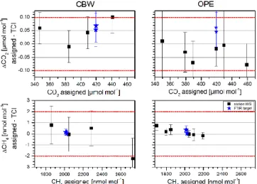
Figure 1 shows the difference between the CAL-assigned concentrations and the TCI measurements for the individual working standards used at the two ICOS stations. At both stations, the assigned concentrations of all working standards are reproduced well by the TCI within the ILC target range of the WMO (0.1 µmol mol−1for CO2and 2 nmol mol−1for CH4), apart from one CBW working standard with a CH4 mole fraction of more than 2700 nmol mol−1. The calibrated CH4 range of the TCI extends only to 2490 nmol mol−1. The observed 1 σ standard deviation of the differences is in accordance with the CO2and CH4reproducibility of the TCI (Hammer et al., 2013). The relatively large error bars for the CH4 differences at CBW are caused by a larger uncertainty of the assigned concentrations. At OPE, the CH4
Fig. 1. Measurement of the CBW (left) and OPE (right) working standards with the TCI at the respective station (black symbols). CO2results are shown in the upper and CH4in the lower panels. The measured means are averages of two times five individual (3 min) TCI measurements; the error bars give the 1 σ uncertainty of the difference accounting for the uncertainties in the assignment as well as the repeatability or the reproducibility (whichever is larger) for the TCI measurements. Blue stars denote differences of the averaged daily TCI target measurements from the CAL-assigned values and their uncertainties at the respective station. Red dashed lines show the WMO ILC target ranges for each species.
calibration comparison exhibits a small concentration de-pendent difference of 0.1 nmol mol−1 per 100 nmol mol−1. This concentration dependence of CH4differences could also explain the observed deviation of 2.2 nmol mol−1 for the highest CBW WS. Thus, a small concentration dependent bias in the CH4 calibration of the TCI seems to be likely. The blue stars in Fig. 1 represent the difference between the CAL assignment and the TCI measurement for the two TCI surveillance/target cylinders regularly used as a repeatability check. The surveillance/target cylinder measurements agree at both stations and in Heidelberg (not shown), within an overall 1 σ standard deviation of 0.06 µmol mol−1 for CO2 and 0.3 nmol mol−1for CH4over the entire 5 months of the ICOS Demonstration Experiment. A detailed presentation of the TCI quality control record, including the station visits at CBW and OPE, can be found in the companion paper by Hammer et al. (2013).
3.2 Sample intake system test (SIS test)
The agreement of the WSs and thus the calibration reference when analysed with one instrument (the TCI) is essential but not in itself sufficient to guarantee compatibility between ambient air datasets from different stations. The ambient air intake system comprises additional hardware, e.g. sample intake tubing, pumps, drying systems etc., which are
potential sources for artefacts. At most stations, the sample intake system is not used for routine cylinder analysis and is also not tested regularly by other measures. To overcome this limitation, the entire sampling path of the ambient air was inspected by the sample intake system test where air from a high pressure cylinder is “sampled” via the ambient air inlet. Performing this test simultaneously for the routine atmospheric monitoring intake and the TCI intake allows for direct comparison of the two independent sample intake systems. Additionally, analysing the same high pressure cylinder at each instrument without the inlet system allows quantification of possible intake system offsets. During the test, the ambient air inlets were connected to a large, elastic buffer volume, which was constantly flushed with air from the high pressure cylinder. A 100 L polyethylene-coated aluminium bag was used as a buffer volume. For more details on the material used and its stability for GHG concentrations we refer to Vogel et al. (2011). The elasticity of the buffer volume ensured that atmospheric pressure conditions were present at the inlet. The humidity of the sample itself was however not comparable to ambient air conditions since predried air from a cylinder was used.
At most stations the sampling lines are constantly flushed at a high flow rate, i.e. several tens of litres per minute, to minimise the residence time of the sample in the inlet line. The actual sample is then tapped off and directed to the analyser using a smaller sample pump. High flow rates constitute a principal problem to the SIS test. Large drainage rates from a high pressure cylinder cause expansion cooling at the regulator of up to 10 K. This cooling can lead to small concentration changes in the decanted gas, most noticeable for CO2 and N2O. We quantified this drainage effect experimentally to be −0.005 ± 0.001 µmol mol−1slpm−1 for CO2and 0.010 ± 0.007 nmol mol−1slpm−1 for CH4. If these observed concentration changes are caused by thermal fractionation as described by Keeling et al. (2007) or whether they result from sorption effects due to different surface conditions on the cold regulator walls is not clear. However, it is a known and now quantified phenomenon that needs to be considered for large cylinder drainage rates. To minimise the cylinder drainage effect (and save gas for analysis), the main line flushing rates had to be reduced (CBW) or line flushing pumps had to be switched off (OPE) during the sample intake test and the intake lines were flushed by the smaller sample pumps only. For all SIS tests the cylinder drainage rate varied between 3 slpm (UHEI) and 7 slpm (OPE). The conditions during the SIS tests were thus not entirely comparable to ambient sampling conditions, but the tests allow for detecting contamination or leaks in the inlet systems and examine the entire sample path.
3.2.1 Sample intake system test Heidelberg
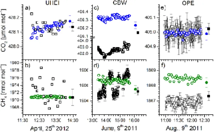
Figure 2a and b show the results of the sample intake test performed in Heidelberg. Open symbols represent the
measurements via the sample intake systems. Filled symbols denote the average and the standard deviation of the direct measurements of the same high pressure cylinder. For CO2 the test measurements of both instruments, the TCI and the GC, agree within 0.02 ± 0.05 µmol mol−1. Moreover, for both instruments, the measurements via the sample intake system agree with the direct measurement of the cylinder. From the latter we can conclude that the Heidelberg intake systems do not introduce significant artefacts. The CH4 results of both instruments led to the same conclusions, although the GC precision for CH4is much worse compared to the TCI (see Fig. 2b).
3.2.2 Sample intake system test CBW
Since the CBW tower is equipped with an elevator that provides easy access to the air intakes, it was possible to attach the buffer volume directly to the inlets of the 200m sampling lines. For the SIS test the line flushing rates of the main pumps were reduced to less than 1 slpm by adjusting the flow controller (CRDS) or closing the respective needle valve (TCI) in the intake system, however the line flushing pumps were kept running. Figure 2c and d show very clearly that the SIS test failed for the CRDS instrument. CO2 measured by the CRDS is lower by 3 to 4 µmol mol−1 compared to the direct measurement and shows large variability of ±0.6 µmol mol−1. CH4 at the same time makes step changes with a standard deviation of ±0.6 nmol mol−1. These differences are too large to be explained by contamination or leaks in the intake system itself and are not in accordance with the ambient air comparison results for CBW (see below). Unfortunately, data evaluation was performed only after the campaign so the test could not be repeated. The most likely explanation for the failure is a leakage in the connection of the CRDS sampling line to the buffer volume.
The simultaneously recorded TCI results agree much better to the direct tank measurements, indicating that the experimental set-up worked as expected for the TCI. The CO2 measurement via the intake system and the direct cylinder measurement differ by 0.09 ± 0.03 µmol mol−1. This difference is too large and of opposite sign to be explained by the cylinder drainage effect. At the applied drainage rate of 7 slpm, the CO2 mole fraction should be depleted by 0.035 µmol mol−1and not enriched. At the same time the CH4 mol fraction is 0.5 nmol mol−1 higher when measured through the TCI intake system. Since the TCI uses the identical drying and sample pumping system as in Heidelberg and OPE, the results suggest that the observed offsets are associated either with the TCI 200 m intake line, their connections or the intake flushing pump. To further examine the origin of this offset an SIS test excluding the long intake line would have been helpful.
The direct cylinder measurements performed with the CRDS are for CO2 0.1 µmol mol−1 and for CH4
Fig. 2. Sample intake system tests at the three stations: Open symbols represent individual measurements via the entire sample intake system, including intake line, pumps and drying systems. Filled symbols denote averaged measurements of the same cylinder without the intake system. Black symbols represent station instru-ment, coloured symbols measurements with the TCI.
0.2 nmol mol−1 lower when compared to the direct TCI measurements. This is not in accordance with the results of the calibration comparison presented in Sect. 3.1 and will be discussed in detail in Sect. 4.1.
3.2.3 Sample intake system test OPE
The results of the SIS tests performed at OPE are shown in Fig. 2e and f. At OPE, the intake system test was performed without the entire 120 m intake line since it was not possible to climb the tower with a heavy high pressure cylinder. Nevertheless, the test included the sampling pumps and the drying systems. The flexible buffer volume of the SIS test was attached at the bottom of the 120 m sampling lines. For both sampling systems the line flush pumps had been switched off and the respective connections were plugged.
For CO2 the agreement between the two intake systems and instruments is nearly perfect with a 0.01 ± 0.06 µmol mol−1 difference. The direct measurements and the measurements via the intake system agree for both instruments well within their respective errors. This implies that neither the drying systems nor the pumps create any significant CO2 artefacts. At the same time the results highlight that the experimental set up of the (restricted) SIS test worked well.
The CH4difference of 1.6 ± 0.4 nmol mol−1between the two intake systems and instruments is however significant. A comparison of the direct cylinder measurements yields already a difference of 0.9 ± 0.4 nmol mol−1. However, the observed CH4 differences cannot be explained by a calibration offset between the two instruments (see Sect. 3.1). The differences between direct and intake system measurement is 0.4 ± 0.4 nmol mol−1 for the CRDS and −0.3 ± 0.4 nmol mol−1 for the TCI. The cylinder used for
the sample intake test was measured at the Heidelberg GC system as well, yielding a CH4 mole fraction of 1868.8 ± 2.4 nmol mol−1, in better accordance with the TCI results. No explanation can be given for the lower CRDS values in the CH4intake sample test.
3.3 Comparison of ambient air measurements
The comparisons of the calibration gases as well as the investigation of the sample intake systems at each station were performed in order to gather diagnostic information for the subsequent evaluation of the ambient air comparison. The results of the comparison of the TCI against the GC at the reference station in Heidelberg are shown in detail in Appendix A. Here, we want to discuss only the results from the comparison experiments at CBW and OPE. These are displayed in a unified manner in Figs. 3 and 4.
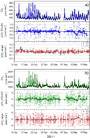
3.3.1 Ambient air comparison CBW
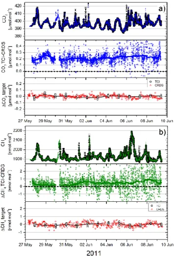
Figure 3 is divided into two similar comparison plots, one for CO2 (panel a) and one for CH4 (panel b). The upper panels in Fig. 3a and b show the 3 min mean values from the TCI in blue and in green, and the 1 min means from the CRDS in black. For CO2, fast changing variations are superimposed on regular diurnal cycles. The CH4 record is dominated by large fluctuations, presumably caused by changing catchment areas. Strong disturbances in the CH4 signal correlate with those in the CO2record. To account for the different temporal resolutions of the two instruments, the CRDS measurements were convoluted with an exponential smoothing kernel representing a 3 min turn-over time. The convolution accounts for the TCI-inherent smoothing in the sample cell, and improves the comparability of the two datasets. The second panels in Fig. 3a and b show the differences between the measurements of the TCI and the CRDS. No data selection was applied. Each open symbol represents one 3 min difference. The filled symbols represent a 4 h running median of the individual differences.
For CO2 the average difference between the two instru-ments varied around 0.2 µmol mol−1; this difference is larger than the WMO-requested ILC target of 0.1 µmol mol−1. The difference is not concentration dependent. The vari-ability of the 3 min differences is generally smaller than ±0.2 µmol mol−1. From 6 June onwards the CO2variability is larger. This is caused by faster concentration changes in the ambient air CO2concentration. In Table 1 the descriptive statistics for the differences is given in more detail. A few outliers are larger than the chosen plot scale. Thus, Table 1 gives the 5th to 95th percentile in order to reflect the range of the typical differences. Potential reasons for the large CO2 offset of 0.21 µmol mol−1between the two instruments will be discussed in Sect. 4.
The smoothed CH4 differences vary between 0 and 1 nmol mol−1, with a slightly increasing trend. The median
Fig. 3. Upper panels in (a) and (b): comparison of CRDS (black) and TCI (blue/green) of CO2 or CH4 measurements performed at the 200 m level at CBW. Middle panels: individual 3 min mean CO2or CH4differences between the TCI and the smoothed CRDS measurements (open symbols); averaged differences (4 h running median filter) as filled symbols. Lower panels: individual 1 min CRDS target measurements in red and individual 3 min TCI target measurements in black. For both instruments the target/surveillance gas deviations are given in a way to allow for direct trend comparison to the ambient air differences.
difference is 0.41 nmol mol−1. The variability of the 3 min differences increases from less than ±1 nmol mol−1 on the first 2 days to ±2 nmol mol−1. The pattern of the increasing variability is comparable to the one from the CO2 compar-ison. The 5th to 95th percentile of the 3 min differences spreads from −0.8 to 1.8 nmol mol−1, highlighting that more than 90 % of the individual 3 min differences are within the WMO-requested ILC target of 2 nmol mol−1.
The lowest panels in Fig. 3a and b show the tar-get/surveillance gas measurements of both instruments. The deviations of the averaged target/surveillance gas concentra-tion minus the 1 min mean CRDS target measurements are shown as open, red symbols. For the TCI the representation is vice versa: 3 min mean TCI target measurements minus
Fig. 4. Upper panels in (a) and (b): comparison of CRDS (black) and TCI (blue/green) of CO2 or CH4 measurements performed at the 120 m level at OPE. Middle panels: individual 3 min mean CO2or CH4differences between the TCI and the smoothed CRDS measurements (open symbols); averaged differences (4 h running median filter) as filled symbols. Note, the first 2 days had to be excluded due to known problems of the CRDS intake system. Lower panels: individual 1 min CRDS CO2or CH4target measurements in red and individual 3 min TCI target measurements in black. For both instruments the target/surveillance gas deviations are given in a way to allow for direct trend comparison to the ambient air differences.
the averaged target/surveillance gas concentration are shown as black, open symbols. This representation of the tar-get/surveillance gas variations was chosen to allow for direct comparison between the trends in the target/surveillance gas records to the ambient air difference. The short term spread of the target/surveillance gas measurements repre-sents the repeatability of the instruments (both instruments: 0.03 µmol mol−1 for CO2 and 0.25 nmol mol−1 for CH4), whereas the consistency over the entire comparison period is a measure for reproducibility. For CO2 as well as for CH4, both instruments measure well within the requested 0.1 µmol mol−1 and 2 nmol mol−1 reproducibility targets for CO2 and CH4 for Northern Hemispheric sites. From
Table 1. Descriptive statistics of the individual CO2 and CH4 differences for the Heidelberg reference station and the two ICOS Demonstration Experiment stations. The median and the inter-quartile range (IQR) of the distributions are given in the first two columns followed by the 5th and 95th percentile. The last two columns state the results of the fitted Gaussian distribution.
median IQR 5th percentile 95th percentile Gauss fit centre Gauss fit std. dev. UHEI (TCI-GC) 1CO2[µmol mol−1] −0.02 0.27 −1.13 1.49 −0.02 0.08 1CH4[nmol mol−1] −0.3 3.6 −5.1 5.1 −0.3 2.3 CBW (TCI-CRDS) 1CO2[µmol mol−1] 0.21 0.09 0.08 0.40 0.21 0.06 1CH4[nmol mol−1] 0.41 0.76 −0.77 1.78 0.38 0.50 OPE (TCI-CRDS) 1CO2[µmol mol−1] 0.13 0.10 −0.02 0.28 0.13 0.07 1CH4[nmol mol−1] 0.44 0.51 −0.28 1.15 0.43 0.36
the repeatability of the two instruments we can estimate the lower limit of the 1 σ variability of the differences to 0.05 µmol mol−1 for CO2 and 0.4 nmol mol−1 for CH4. Any potential variability originating from the sample intake system as well as temporal misalignments adds to this. None of the target/surveillance gas records holds evidence for instrumental drifts during the comparison period. The CRDS target/surveillance gas records show small diurnal patterns that are more distinct for CO2. The inter-diurnal variability in the smoothed CH4 differences is to some extent present in the CRDS target/surveillance gas variability, however, no explanation for the slight temporal increase of the CH4 differences between the TCI and the CRDS can be drawn from the target/surveillance gas records and thus from the analyser performance and calibration.
3.3.2 Ambient air comparison OPE
Figure 4 shows the results for the OPE comparison campaign and is structured identically to Fig. 3. The upper panels in Fig. 4a and b, respectively, present the 3 min mean CO2 (blue) and CH4(green) measurements of the TCI and compares them to the 1 min mean measurements of the CRDS (black). During the first 3 days of the two weeks comparison campaign no adequate CRDS data is available due to experimental problems with the ICOS prototype. As for CBW, the CRDS measurements have been convolved with the exponential kernel before calculating the differences between the two instruments shown in the middle panels in Fig. 4a and b. The individual 3 min differences are shown as open symbols and have been smoothed using a 4 h running median filter shown as filled symbols. For CO2the smoothed differences vary between 0.1 and 0.2 µmol mol−1 with a median difference of 0.13 µmol mol−1. The scatter of the individual differences is on the order of ±0.15 µmol mol−1. This is also expressed by the 5th and 95th percentile given in Table 1. The observed median CO2 difference between the TCI and the CRDS is again larger than the WMO-requested
ILC target and discussed in more detail in Sect. 4.2. The smoothed CH4 differences decrease from initially 0.7 nmol mol−1to 0.1 nmol mol−1. The median difference is 0.4 nmol mol−1. Despite this trend the individual differences are generally well in line with the WMO-requested ILC target. Even the 5th and 95th percentile of the 3 min differences, as given in Table 1, is well below the requested compatibility ranges.
The individual target/surveillance gas measurements of both instruments are shown in the lower panels in Fig. 4a and b. As already mentioned in Sect. 3.1 the TCI performance for CO2 was worse at OPE than at CBW. This was due to large temperature variations (10 K) within the measurement container and a slowly deteriorating flow controller in the TCI instrument, decreasing the CO2 reproducibility to 0.07 µmol mol−1. For more details on the performance of the FTIR during this period see the companion paper by Hammer et al. (2013). Also, the CO2 repeatability of the CRDS system in OPE was worse (1 σ = 0.08 µmol mol−1) than that at CBW, which is explained by the earlier CRDS version running at OPE compared to CBW (see Sect. 2.2). Both effects can be seen in the scatter of target/surveillance gas measurements displayed in Fig. 4a and b. The TCI’s repeatability as well as its reproducibility are affected. For CH4the TCI target measurements show a decreasing trend of 0.6 nmol mol−1over the two weeks period. This trend is in accordance to the observed decrease of the CH4differences and attributes it entirely to the performance of the TCI at OPE. For both CO2 and CH4 CRDS target/surveillance gas records, an initial settling in effect is detectable, which disappears after the first 3 days when the actual comparison measurements start. The TCI CO2 target shows variations that are larger than the WMO ILC ranges; this indicates poor reproducibility. In contrast to CH4, no direct relation to the ambient air difference of CO2is visible. The variability in the TCI CO2 target/surveillance gas measurements is even larger than the observed variability in the ambient
air differences. This is related to the deteriorating flow controller of the TCI, which caused longer stabilisation times. These increased settling-in effects are more severe for limited 30 min target/surveillance gas measurements than for the continuous ambient air measurements. It was generally observed that the TCI performance with CO2is much more affected from non-stable conditions than with CH4(Hammer et al., 2013).
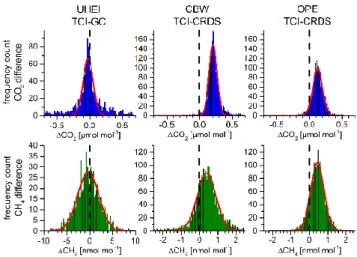
3.4 Statistical evaluation of ambient air measurements Since for all sites the CO2 and CH4 differences are not Gaussian distributed, the results are presented in separate histograms in Fig. 5 (for individual measurements of Heidelberg see Appendix A). A non-Gaussian distribution results if systematic errors are present. Sources of systematic errors could be numerous, e.g. drifts in one of the instru-ments, temporal misalignments among the instruments or incorrect calibrations/response functions. The WMO ILC targets are stated as standard deviations without specifying the distribution of the population (WMO, 2011), with the tacit understanding of the Gaussian distribution. However, the range covered by the standard deviation is distribution dependent. For example, one standard deviation of the CO2 difference at CBW (Fig. 3a) includes 94 % of all data. Thus we chose the inter-quartile range, a distribution independent measure, to quantify the spread of the data (Borradaile, 2003). Since it is common to report the standard deviation, we also report the standard deviation of a Gaussian fit to the histogram for comparison reasons. The IQR is far less sensitive to outliers, thus no data flagging needs to be applied, reducing randomness in selecting the flagging criteria and the effort in data preprocessing. The graphical representation of the histogram in combination with a fitted Gaussian distribution, as given in Fig. 5, acts as an easy check of normality and highlights the presence and the extent of potential systematic errors.
Table 1 summarises the results of the TCI comparison to the standard instrumentation at the Heidelberg reference site and the two ICOS Demonstration Experiment sites. In addition to the median and the IQR, the parameters of the Gauss fit of the distributions as well as the 5th and 95th percentiles are given. The median differences of the TCI relative to the Heidelberg reference GC are −0.02 µmol mol−1for CO2and −0.3 nmol mol−1for CH4; the compatibility is thus well within the WMO-requested ILC targets for both gases. The large IQR value for CO2 and the obvious mismatch between the CO2 histogram and its Gauss fit are probably caused by the large variability of ambient air concentrations in combination with a temporal misalignment of the two instruments in Heidelberg (see Fig. A1). The differences between the TCI and the GC are largest and most distinct for periods with fast concentration changes. For a more detailed discussion on this topic see Appendix A. The same temporal misalignment problem is
Fig. 5. Histograms of the individual CO2 (upper panel) and CH4(lower panel) differences for the different stations. For each histogram a Gaussian distribution is fitted and given in red. Note the different scale for CH4in Heidelberg.
present for the CH4 differences. However, the temporal misalignment problem is masked by the CH4precision of the GC system (±2.3 nmol mol−1), which constitutes the lower limit for the variability of the differences and is exemplified in Fig. 5. Since this statistical error of the CH4 difference is already large it masks the systematic error. Thus the deviation of the CH4 histogram from the Gauss fit is much smaller. From the good, absolute agreement between the GC and the TCI we can conclude that it is possible to use the TCI in its current set-up to assess the performance of a field station.
The variability of the differences is much smaller at the two field stations compared to that at the Heidelberg reference station. This has two reasons: first, the temporal resolution of the CRDS is 1 min and can, after proper smoothing, be more accurately compared with the 3 min data of the TCI; and secondly, the variability of the ambient concentrations in CBW and OPE are much smaller than in Heidelberg. For CBW only small deviations from the Gauss fit, mainly for positive differences, are found. These deviations originate from a small increasing trend in the CO2 and CH4difference (compare Fig. 3), accompanied with an increasing variability of the differences. Still, at both field stations, the variability of the differences, either expressed as IQR or as standard deviation of the Gauss fit, is smaller than the WMO ILC target. This highlights the potential of the parallel measurement approach, even without flagging any data points and without restricting the comparison to clean air or baseline conditions. The agreement between the instruments in terms of precision is remarkable. For CH4the accuracy between the different measurement systems is also sufficient to fulfil the WMO ILC target. However, for CO2 none of the measurements at the two field stations agrees with those of the TCI within the required limits.
4 Discussion of comparison results and suggestions for improvements
In the following section we will compare all our results, i.e. of direct calibration standard measurements, SIS tests, if available, and parallel ambient air measurements at the ICOS Demonstration Experiment sites and try to understand the ob-served differences of ambient CO2and CH4measurements. For this purpose Table 2 combines the results of all tests performed at the field stations. In addition, we will discuss some of the misconceptions during this inter-comparison exercise that should be avoided in the future.
4.1 CBW comparison
The sample intake test at CBW was only successful for the TCI and showed a 0.09 ± 0.03 µmol mol−1higher CO2value when the cylinder gas passed through the complete intake system of the TCI compared to the direct measurement. If the same bias would occur for real ambient air measurements at the TCI, this would explain about half of the observed ambient air difference of 0.21 µmol mol−1. The TCI mea-sured the SIS test gas higher by 0.10 µmol mol−1 when compared to the CRDS instrument. Both effects together would account for the difference observed between the ambient CO2measurements at Cabauw. However, the result of the direct SIS test cylinder appears to contradict the results of the calibration gas comparison. Compared with the CAL-assigned values of the CBW working standards (Table 2) the TCI values were lower by 0.05 µmol mol−1. This contradiction points to some bias of the instrument calibration at Cabauw. In-depth investigation of the 1 min CRDS measurements of the test gas at CBW showed that the CO2concentration does not reach a steady value within the measurement interval of 5 min, which was chosen for cylinder gas analysis (Vermeulen et al., 2011). This may be caused by settling in effects of regulators and/or insufficient flushing of dead volumes in the calibration gas inlet system. The same problem occurs for the WSs, which are also flushed for only 5 min every 25 h. The insufficient flushing of the WSs affects the Licor NDIR CO2 measurements as well. In the meantime the measurement duration for the WSs has been increased to 15 min.
For CH4, the observed calibration offsets and the bias in the TCI SIS test are in accordance with the observed mean ambient air difference between the instruments. In addition, the calibration gas differences derived from the CBW WS measurements on the TCI and the offset between the direct measurements of the intake test cylinder agree within their uncertainties. This result is not in contradiction with the insufficient WS flushing that we observed for CO2, since pressure regulator effects are known to be much smaller for CH4than for CO2. This is also supported by the fact that CH4 reached its equilibrium value within the 5 min flushing time.
The TCI SIS test results for both species are higher if measured via the intake system. The ambient CO2 and CH4concentrations measured directly prior to the SIS test were lower compared to those of the SIS test cylinder; thus, potential leaks in the SIS test set-up are not a likely explanation for the observed difference. However for both species elevated concentration levels are very likely to be present within the station building. Therefore leakages at the connection of the sample line to the TCI or at the TCI line flushing pump are possible explanations. Retrospectively, an SIS test without the sample intake line would have been helpful to further narrow down the source of the discrepancies.
4.2 OPE comparison
The median CO2offset at OPE between the two instruments (0.13 µmol mol−1) is also larger than the WMO ILC target. The calibration difference between the instruments can only account for 0.03 µmol mol−1. The “restricted” sample intake system test did not show any differences between the two instruments for CO2. This leads to the conclusion that the pumps and the drying systems of both instruments probably do not cause any systematic offset. Thus, 0.10 µmol mol−1 of the CO2 difference remains unexplained. Due to lo-gistical problems it was not possible to test the intake lines at OPE. Thus the untested lines and potentially the line flushing pumps might have caused the unexplained differences. The differences are of similar size compared to the 0.09 µmol mol−1 difference that was found during the TCI SIS test at CBW. Since the TCI and the CRDS sample line are made of identical 1/200Synflex 1300 material and the lines have been flushed at similar rates, different contaminations of the two lines are not very likely. It would be in accordance with all our test results if the TCI line flushing pump would have caused this 0.10 µmol mol−1 offset. The pump (Becker, VT 4.4) was, however, never tested for contamination since it was placed downstream of the entire sample intake system.
The median ambient air CH4 offset at OPE is 0.44 nmol mol−1and thus well within the WMO ILC target. However, the results of the SIS test and the ambient air comparison are not in accordance. From the sample intake system test we would have expected a difference of 1.6 nmol mol−1 between the two systems (see Fig. 2f). Detailed investigation of both the CRDS and the TCI results of the CH4SIS test could not explain this discrepancy.
4.3 Summary of differences
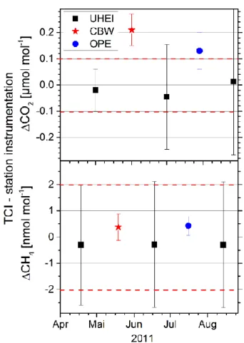
Figure 6 summarises the observed ambient air differences between the TCI and instrumentation at its reference station Heidelberg and at the two field stations CBW and OPE. Before and after each field trip, the TCI was checked against the Heidelberg GC system to reassure that its performance
Table 2. Overview of the different comparison tests performed at the ICOS field stations. The representation of the test results is presented with respect to their sign, to be directly comparable to the observed ambient air difference.
Differences
Calibration: SIS SIS test SIS test ambient
TCI- cylinders CRDS: TCI: air:
assigned TCI-CRDS direct-line line-direct TCI-CRDS CBW 1CO2[µmol mol−1] −0.05 ± 0.05 0.10 ± 0.02 – 0.09 ± 0.03 0.21 ± 0.06 1CH4[nmol mol−1] −0.4 ± 0.4 0.2 ± 0.3 – 0.5 ± 0.2 0.4 ± 0.5 OPE 1CO2[µmol mol−1] 0.03 ± 0.04 0.03 ± 0.04 0.02 ± 0.05 0.00 ± 0.06 0.13 ± 0.07 1CH4[nmol mol−1] −0.2 ± 0.3 0.9 ± 0.4 0.4 ± 0.4 0.2 ± 0.3 0.4 ± 0.4
did not change. For both species, CO2 and CH4, the TCI and the Heidelberg GC did agree before, in between, and after the field trips to CBW and OPE. The averaged differences between the UHEI GC and TCI did not change significantly. This finding, in combination with a smooth TCI target/surveillance gas record (Hammer et al., 2013), gives confidence that the TCI remained stable over the time of the Demonstration Experiment and can thus serve as reference instrument for both station visits. The generally larger and increasing variability of the CO2 differences relative to the GC system are discussed in Appendix A and can be explained by temporal misalignment between the two instruments.
The CO2 deviations at CBW can possibly be partly explained by an offset caused by the TCI intake line or the line flushing pump and the systematic error of the CRDS calibration caused by insufficient flushing of the working standards. At OPE, the CO2 deviations are smaller than at CBW and close to the WMO target; however, no explanation for the significant difference could be found. The only parts that remain essentially untested at OPE are the sample intake lines. Dedicated tests of the intake lines have to be carried out at both stations in order to clarify, i.e. if the 0.09 µmol mol−1 contamination, which we have found for the TCI sampling line in CBW, is indeed reproducible and of the same size when ambient air measurements are performed and if the CO2offset observed between the two instruments at OPE is actually caused by a similar line effect.
The CH4deviations at CBW and OPE are of the same size and both smaller than the limit of the ILC target.
4.4 Critical assessment of the comparison experiment and suggestions for improvements
The feasibility study of using a travelling instrument to detect differences in the order of the WMO ILC target was successful. The high precision of the two optical instruments used in the comparison, i.e. the FTIR and the CRDS, allowed us to even detect small differences in the co-located
Fig. 6. Summary of the differences of atmospheric measurements and their 1 σ standard deviations (Gauss fit) between the TCI and the respective stations for CO2 (upper panel) and CH4 (lower panel).
measurements over a short comparison period of one to two weeks. Significant offsets can also be detected on even smaller timescales like, e.g. hours. The approach is truly comprehensive since ambient air collected from the same inlet point is compared. In contrast to earlier studies, our data evaluation method allows us to compare the entire
ambient concentration range so that we are not restricted to background conditions, only. With the dedicated component tests, like the SIS test and the calibration check, the travelling instrument approach represents a true diagnostic evaluation directly at the field station under its potentially unique conditions. The travelling instrument approach is, however, labour intensive, since the TCI has to be referenced to independent instrumentation at its home base before and after each field trip. This reduces the comparison capacity of one TCI to only four or five station visits per year. From our experience, conducting the TCI approach, including preparation and data evaluation, would need the capacity of one fulltime scientist, at least during the first year. In addition, as long as the FTIR is used as TCI, the campaigns have to be supported by a technician or a student helper. A smaller and lighter instrument can be installed by only one person.
Evaluation of the feasibility study has demonstrated the potential of such an approach, but at the same time improvements are needed:
– First and foremost, near-real time data evaluation is a key requirement. Calibrated data from both instru-ments must be available within 24 h during an inter-comparison campaign. This will allow for quickly reacting to experimental problems, e.g. realise the necessity to repeat the sample intake test at CBW. Due to delays at the start of the ICOS Demonstration Experiment, the travelling instrument campaign took place right at the beginning of this ICOS phase where the data processing chains between the field stations and the ICOS Atmospheric Thematic Centre, responsible for processing the continuous data, had not yet been fully operational. Thus, CRDS data were only available a few weeks after the station visits.
– The example of insufficient flushing times in the CBW set-up has shown that a check of the station’s calibration standards with the travelling instrument is not sufficient. Measuring the TCI working standards at the station instrument will give additional information on how well the scale is transferred from the station calibration standards to the station instrument. Our approach was vice versa and thus checked the accordance of the two standard sets and the scale transfer to the TCI. In our comparison we had only one direct cylinder comparison at both instruments, which already highlighted a respec-tive problem.
– For future TCIs it will be mandatory for the TCI host laboratory to have a separate intake line for the TCI instrument and to use the same line flushing pump as during the field comparisons.
5 Possible quality management strategies for a network of continuous analysers
5.1 Requirements for a comprehensive quality management strategy
The travelling instrument approach evaluated in this study could be part of an overall quality management of continuous atmospheric monitoring stations. The requirements for such a comprehensive quality management (QM) of a network are complex. Thus, multiple tools will be needed to cover various aspects. In the following, we will briefly outline the key points that should be addressed when designing such a quality management system:
– Precision: the precision of the quality management tool defines the needed statistics to detect differences on the order of the WMO ILC goals. Preferably, the precision of a QM tool should be at least twice the requested ILC targets (WMO, 2012).
– Frequency: comparison frequency must allow for quickly detecting potential problems.
– Comprehensiveness: it must describe, which parts of the analytical set-up are tested.
– Concentration range coverage: it should be suitable for the investigated station and slightly exceed the stations ambient concentration range.
– External station validation: this quality control item is mandatory to create credibility of the network data.
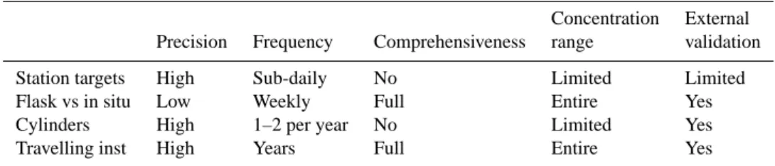
Table 3 summarises quality control (QC) techniques that could be applied to field stations and classifies them according to the previously defined quality management characteristics. Each QC technique mentioned has its own strengths and weaknesses.
In the last decades, regular target/surveillance gas mea-surements have proven invaluable to monitor and quantify instrument performance. Target gases can be measured very precisely and at a high frequency. Thus target/surveillance gas measurements will form the backbone of the QM in order to be able to react timely on any instrumental malfunction including drifts in WS. The major shortcoming of the target/surveillance gases is that they are not comprehensive and test only the instrument response but not the air intake system. To overcome this problem, we propose to use multiple targets and multiple insertion points for one of these targets. In addition to the usual insertion point, e.g. at the sample selection valve, a second insertion point prior to a potential pump and/or drying system is proposed. Such an alternative target/surveillance gas insertion point was already proposed by Stephens et al. (2011). In our set-up we propose to alternate one of the target/surveillance gases between the two insertion points and thus direct the gas through
Table 3. Classification of existing quality management approaches according to the predefined quality management characteristics Concentration External
Precision Frequency Comprehensiveness range validation
Station targets High Sub-daily No Limited Limited
Flask vs in situ Low Weekly Full Entire Yes
Cylinders High 1–2 per year No Limited Yes
Travelling inst High Years Full Entire Yes
parts of the sample intake system, such as, e.g. the drying system and/or the sample pumps. Performing such tests on a weekly to monthly basis in addition to regular direct target measurements will improve the comprehensiveness of the target/surveillance gas measurements enormously. We propose to use yet an additional target/surveillance gas cylinder to check the intake system since gas consumption will be high. However, even this extended target/surveillance gas concept can still not provide an adequate external validation of the compatibility of the station measurements. Target gases can be calibrated by an external body prior and after usage and thus represent some external validation but with very little temporal coverage.
Concurrent flask sampling could fill this gap. Regular, e.g. weekly flask samples, which are analysed at a different laboratory and compared to the in situ measurements provide the needed external validation. Up to now, the 1 σ variability of flask versus in situ comparisons are on the order of 0.3 to 0.8 µmol mol−1 for CO2 (Masarie et al., 2011a, b), therefore, many single comparisons are needed to achieve the desired precision of inter-laboratory biases. However, the variability of the flask in situ comparisons is expected to improve, once flasks can be filled over an extended, well defined, period (e.g. 1 h by using a buffer volume) as proposed recently by Turnbull et al. (2012). This should make the flask sample more representative and will ease the comparison to continuous ambient measurements. The flask in situ comparison will cover the entire concentration range at the station and will thus allow one to investigate concentration dependencies of biases.
Especially if the flask measurements and the in situ measurements are performed within the same measurement network, it is strongly recommended to also introduce a network-external QC measure. Such comparisons could be similar to today’s WMO round robin (Zhou et al., 2011) exercise or the European “cucumber” ICP (Manning et al., 2009) and can be performed on a lower frequency. The important aspect is that they have to be completely independent from the network they are monitoring.
True comprehensiveness is only established via a com-pletely independent measurement that includes the air sampling system, such as the flask in situ comparison. In order to have a second comprehensive check of the whole system we propose to perform a sample intake system test,
at least after setting up a new station, and regularly, e.g. once per year.
The TCI is an alternative, completely independent and comprehensive QC measure. In contrast to concurrent flask sampling analysis, this approach is capable of detecting small discrepancies, even on a sub-hourly timescale. We propose thus to use the TCI as a diagnostic tool within a monitoring network. Its travel route should however be flexible and be decided based on the results of the other QM measures.
5.2 Proposed quality management strategy for a monitoring network with continuous high precision analysers
1. Complete check of all intake lines before a station becomes operational. If the intake line of a station is made of Synflex and has connectors that are exposed to the weather this line test should be repeated at a regular interval.
2. High frequency of instrument target/surveillance gas measurements at the station to be able to quickly detect malfunctioning of the instrument; insertion point: selection valve (at least daily).
3. Low frequency of instrument target/surveillance gas measurements to be able to quantify system stability over decades; insertion point: selection valve.
4. Low frequency (e.g. weekly) intake target/surveillance gas measurements with two insertion points: (a) selec-tion valve, (b) prior to drying system and pump.
5. Regular flask – in situ comparison: weekly.
6. Travelling cylinders (highest hierarchy, ideally cali-brated by the WMO CCL) to check calibration scales. This should be carried out as a blind test every 2 yr.
7. The travelling instrument serving as a diagnostic tool particularly for stations where systematic biases in the flask vs in situ comparison occur.
The QM strategy as proposed above does fulfil all needs in terms of precision, frequency, concentration range coverage, external validation, as well as comprehensiveness. The di-versity of the applied QC measures complement one another
and offer sufficient redundancies to act as a defensible QM system. Technical restrictions at the monitoring site or other constraints may impede the implementation of the entire scheme. In any case we would advise to have at least the high frequency target/surveillance gas measurements and the regular flask – in situ comparison.
6 Conclusions
The approach of using a travelling comparison instrument as a quality control measure was successfully tested at two field stations for CO2 and CH4. The TCI approach has proven to be sufficiently precise to detect differences between the measurement systems, which are well below the WMO ILC targets. Even on a 3 min temporal resolution the spread, measured either as IQR or fitted standard deviation, of the differences between the FTIR and CRDS instruments is smaller than the ILC target. This allows for very detailed (e.g. hourly) investigation of the differences. For such high-resolution comparisons an extended definition of the ILC target would be desirable, adding variance limits to the current offset limits. These variance limits should be defined in close cooperation with the inverse modelling community and should anticipate the scientific needs and the capacity of future fine-grid models. Ideally, these variance limits should be defined in a distribution independent manner.
The combination of the TCI with the dedicated test of the instrument components like the calibration check and the SIS test allow for subdivided testing of individual components of the measurement device. The proposed SIS test constitutes, besides co-located flask sampling, the only comprehensive test of the entire instrument system. Despite the experimental problems that we encountered in this feasibility study the SIS test has a high diagnostic potential. However, it also showed that more work and on-site evaluation of the results by the station team in cooperation with the TCI team is required to eliminate observed biases after they have been diagnosed. The results of this study highlight the demand for truly comprehensive QC. The proposed QM strategy could fulfil the diverse requirements and provide sufficient redundancy to establish traceable and defensible data quality standards.
Appendix A
Remark on the CO2variability and temporal
representativeness of the Heidelberg GC
measurements and their comparability with the TCI data Depending on the measurement principle and instrumenta-tion, different temporal resolutions of ambient air measure-ments are achieved. Classical GC systems have a sampling frequency of 5 to 15 min, and the measurement represents a snap-shot of the currently sampled atmospheric condition. The averaging time of the in situ FTIR instrument is 3 min,
Fig. A1. Upper panels of (a) and (b): comparison of GC (black) and TCI (blue/green) of CO2 or CH4 measurements performed in Heidelberg. Middle panels: individual CO2or CH4differences between the buffered GC and the smoothed TCI measurements (open symbols); averaged differences (15 h running median filter) are shown as filled symbols. The smoothing window is larger, compared to the ICOS Demonstration Sites, to account for the lower comparison frequency of the individual measurements. Lower panels: individual CO2 or CH4 GC target injections in red and individual TCI target measurements in black.
which corresponds to the turn over time τ of the white cell in the spectrometer (Hammer et al., 2013). The large, white cell of the FTIR smoothes the high frequent variability in atmospheric trace gases that might be captured by the snap-shot type measurement of the GC system. Especially for polluted or semi-polluted stations close to GHG sources this leads to a representativeness difference between the measurement systems. To increase the representativeness of the snap-shot like GC measurements, a spherical 10 L buffer volume was introduced in the GC sampling line. A detailed description of the buffer volume concept can be found in Winderlich et al. (2010). In the Heidelberg GC
![[PDF] Initiation au développement Qt sur les sockets | Cours informatique](data:image/gif;base64,R0lGODlhAQABAIAAAP///wAAACH5BAEAAAAALAAAAAABAAEAAAICRAEAOw==)