The potential to narrow uncertainty in projections of stratospheric ozone over the 21st century

(1)

HAL Id: hal-00482182

https://hal.archives-ouvertes.fr/hal-00482182

Submitted on 5 Jan 2016

HAL is a multi-disciplinary open access

archive for the deposit and dissemination of

sci-entific research documents, whether they are

pub-lished or not. The documents may come from

teaching and research institutions in France or

abroad, or from public or private research centers.

L’archive ouverte pluridisciplinaire HAL, est

destinée au dépôt et à la diffusion de documents

scientifiques de niveau recherche, publiés ou non,

émanant des établissements d’enseignement et de

recherche français ou étrangers, des laboratoires

publics ou privés.

stratospheric ozone over the 21st century

Andrew J. Charlton-Perez, E. Hawkins, V. Eyring, I. Cionni, G. E. Bodeker,

D. E. Kinnison, H. Akiyoshi, S. M. Frith, R. Garcia, A. Gettelman, et al.

To cite this version:

Andrew J. Charlton-Perez, E. Hawkins, V. Eyring, I. Cionni, G. E. Bodeker, et al.. The potential to

narrow uncertainty in projections of stratospheric ozone over the 21st century. Atmospheric Chemistry

and Physics, European Geosciences Union, 2010, 10 (19), pp.9473-9486. �10.5194/acp-10-9473-2010�.

�hal-00482182�

(2)

www.atmos-chem-phys.net/10/9473/2010/ doi:10.5194/acp-10-9473-2010

Chemistry

and Physics

The potential to narrow uncertainty in projections of stratospheric

ozone over the 21st century

A. J. Charlton-Perez1, E. Hawkins1, V. Eyring2, I. Cionni2, G. E. Bodeker3, D. E. Kinnison4, H. Akiyoshi5, S. M. Frith6, R. Garcia4, A. Gettelman4, J. F. Lamarque4, T. Nakamura5, S. Pawson7, Y. Yamashita5, S. Bekki8, P. Braesicke9, M. P. Chipperfield10, S. Dhomse10, M. Marchand8, E. Mancini11, O. Morgenstern12, G. Pitari11, D. Plummer13, J. A. Pyle9, E. Rozanov14,15, J. Scinocca13, K. Shibata16, T. G. Shepherd17, W. Tian10, and D. W. Waugh18

1_{University of Reading, Dept. of Meteorology, Reading, UK}

2_{Deutsches Zentrum für Luft- und Raumfahrt, Institut für Physik der Atmosphäre, Oberpfaffenhofen, Germany} 3_{Bodeker Scientific, The Elms, Alexandra, New Zealand}

4_{National Center for Atmospheric Research, Boulder, CO, USA} 5_{National Institute for Environmental Studies, Tsukuba, Japan} 6_{Science Systems and Applications, Inc., Lanham MD 20706, USA} 7_{NASA Goddard Space Flight Center, Greenbelt, Maryland, USA} 8_{Service d’Aeronomie, Institut Pierre-Simone Laplace, Paris, France} 9_{University of Cambridge, Department of Chemistry, Cambridge, UK} 10_{University of Leeds, Institute for Atmospheric Science, UK} 11_{Universit L’Aquila, Dipartimento di Fisica, L’Aquila, Italy}

12_{National Institute of Water and Atmospheric Reasearch, Lauder, New Zealand} 13_{Environment Canada, Victoria, BC, Canada}

14_{Physikalisch-Meteorologisches Observatorium Davos/World Radiation Center, Davos, Switzerland} 15_{Institute for Atmospheric and Climate Science ETH, Zurich, Switzerland}

16_{Meteorological Research Institute, Tsukuba, Japan} 17_{University of Toronto, Department of Physics, Canada}

18_{Johns Hopkins University, Department of Earth and Planetary Sciences, Baltimore, Maryland, USA}

Received: 25 March 2010 – Published in Atmos. Chem. Phys. Discuss.: 6 May 2010 Revised: 9 July 2010 – Accepted: 20 August 2010 – Published: 7 October 2010

Abstract. Future stratospheric ozone concentrations will be

determined both by changes in the concentration of ozone depleting substances (ODSs) and by changes in stratospheric and tropospheric climate, including those caused by changes in anthropogenic greenhouse gases (GHGs). Since future economic development pathways and resultant emissions of GHGs are uncertain, anthropogenic climate change could be a significant source of uncertainty for future projections of stratospheric ozone. In this pilot study, using an

“ensem-Correspondence to: A. J. Charlton-Perez

(a.j.charlton@reading.ac.uk)

ble of opportunity” of chemistry-climate model (CCM) sim-ulations, the contribution of scenario uncertainty from dif-ferent plausible emissions pathways for ODSs and GHGs to future ozone projections is quantified relative to the contri-bution from model uncertainty and internal variability of the chemistry-climate system. For both the global, annual mean ozone concentration and for ozone in specific geographical regions, differences between CCMs are the dominant source of uncertainty for the first two-thirds of the 21st century, up-to and after the time when ozone concentrations return up-to 1980 values. In the last third of the 21st century, depen-dent upon the set of greenhouse gas scenarios used, sce-nario uncertainty can be the dominant contributor. This result

(3)

suggests that investment in chemistry-climate modelling is likely to continue to refine projections of stratospheric ozone and estimates of the return of stratospheric ozone concentra-tions to pre-1980 levels.

1 Introduction

Over the past four years the chemistry-climate modelling community has made progress in understanding and refin-ing projections of stratospheric ozone over the 21st century. For the first time, a large number of Chemistry-Climate Mod-els (CCMs) have been run using common ozone and climate forcings for the period 1960–2100 for the second phase of the Stratospheric Processes And their Role in Climate (SPARC) Chemistry-Climate Model Validation Project (CCMVal2). The set of model integrations provided by 18 modelling cen-tres around the world has been extensively studied by a large number of authors and a comprehensive report detailing our current understanding of the CCMs was completed early in 2010. As part of CCMVal2, a new analysis of uncertainty in projections of total column ozone over the 21st century and dates of return of total column ozone has been produced (Chapter 9, SPARC CCMVal, 2010). This analysis, how-ever, has been conducted for reference simulations of CCMs based on a common GHG forcing scenario. Many recent studies have pointed to the role that future changes in GHG concentrations might play in determining both global and re-gional ozone abundances over the 21st century (Shepherd, 2008,Waugh et al., 2009, Jonsson et al., 2009, Oman et al., 2010a). GHGs can affect ozone concentrations through the additional HOxand NOxproduction from increases in CH4

and N2O decomposition, through acceleration of catalytic

ozone destruction cycles in the colder stratosphere and in-directly by influencing the strength of the Brewer-Dobson circulation and hence the meridional and vertical transport of ozone (Barnett et al., 1974; Randeniya et al., 2002; Rosen-field et al., 2002; Haigh and Pyle, 1982; ChipperRosen-field and Feng, 2003; Portmann and Solomon, 2007; Ravishankara et al., 2009; Butchart et al., 2006).

Given the sensitivity of ozone amounts to GHG concen-trations, there is an additional uncertainty in projections of ozone column amounts due to the uncertainty in the use of fossil fuels and other GHG producing compounds over the next 100 years. In the climate change community, this un-certainty is addressed by producing projections of climate variables using a range of different possible GHG scenarios (Special Report on Emissions Scenarios, Nakicenovic et al. (2000)), consistent with economic models of global devel-opment. While these scenarios do not necessarily span the full range of possible GHG emissions, they do at least allow an estimate of the sensitivity of climate models to different economic development paths.

In this study, additional simulations of the CCMs used for the CCMVal2 intercomparison forced with different GHG scenarios (and in some cases slightly different ODS

scenar-ios) are used to quantify the uncertainty in global and re-gional stratospheric ozone projections associated with three factors: model uncertainty, scenario uncertainty and internal variability. By separating the overall uncertainty of CCM projections in this way, it is possible to identify regions in which:

– model uncertainty is dominant, such that projections

could be improved by CCM development leading to a narrowing of this uncertainty,

– scenario uncertainty is dominant, such that additional

simulations of CCMs forced with different GHG scenar-ios would enable a better understanding of future ozone abundances, and

– internal variability is relatively large, such that there

will be significant component of the total uncertainty which is irreducible.

Identifying regions and time periods where these conditions are found will aid future CCM ensemble design and inform policymakers about the potential to narrow uncertainty in ozone projections.

2 Model integrations

Model integrations used in this analysis form part of the CCMVal2 intercomparison project. The core set of integra-tions used are so-called future reference simulaintegra-tions (REF-B2) from the CCMVal2 activity. These simulations are de-scribed and assessed in detail in the SPARC CCMVal report (SPARC CCMVal, 2010) and the participating CCMs are de-scribed in Morgenstern et al. (2010) and references therein. REF-B2 simulations use surface time series of halocarbons based on the adjusted A1 scenario from WMO (2007), and the long-lived GHG concentrations are taken from the SRES A1b scenario Nakicenovic et al. (2000). Sea surface tem-peratures (SSTs) and sea ice concentrations (SICs) are gen-erally prescribed from coupled ocean model simulations, ei-ther from simulations of the same atmospheric Global Cir-ulation Model (GCM) run with a coupled ocean, or from coupled ocean-atmosphere model simulations of a different AR4 GCM simulation under the same A1B GHG scenario. Only one of the 13 CCMs used here ran with a coupled ocean (CMAM).

To avoid artifacts from using different numbers of mod-els as time progresses (Chapter 9 of SPARC CCMVal, 2010; Waugh and Eyring, 2008), only the subset of 13 CCMVal REF-B2 simulations that provided output from 1960–2095 are used in this study.

In addition to these REF-B2 simulations, several other model integrations which primarily varied the GHG scenario are also analysed. Five different GHG scenarios are con-sidered, with the models running each scenario listed in Ta-ble 1. Two scenarios were run with different SRES pathways

(4)

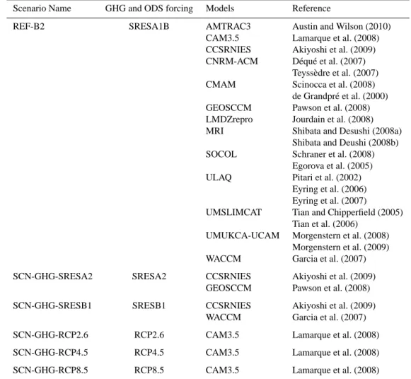
Table 1. Simulations used in the analysis.

Scenario Name GHG and ODS forcing Models Reference

REF-B2 SRESA1B AMTRAC3 Austin and Wilson (2010)

CAM3.5 Lamarque et al. (2008)

CCSRNIES Akiyoshi et al. (2009)

CNRM-ACM D´equ´e et al. (2007)

Teyss`edre et al. (2007)

CMAM Scinocca et al. (2008)

de Grandpr´e et al. (2000)

GEOSCCM Pawson et al. (2008)

LMDZrepro Jourdain et al. (2008)

MRI Shibata and Desushi (2008a)

Shibata and Deushi (2008b)

SOCOL Schraner et al. (2008)

Egorova et al. (2005)

ULAQ Pitari et al. (2002)

Eyring et al. (2006) Eyring et al. (2007)

UMSLIMCAT Tian and Chipperfield (2005)

Tian et al. (2006)

UMUKCA-UCAM Morgenstern et al. (2008)

Morgenstern et al. (2009)

WACCM Garcia et al. (2007)

SCN-GHG-SRESA2 SRESA2 CCSRNIES Akiyoshi et al. (2009)

GEOSCCM Pawson et al. (2008)

SCN-GHG-SRESB1 SRESB1 CCSRNIES Akiyoshi et al. (2009)

WACCM Garcia et al. (2007)

SCN-GHG-RCP2.6 RCP2.6 CAM3.5 Lamarque et al. (2008)

(SRESA2 and SRESB1) but with an identical ODS scenario to the standard REF-B2 runs. Three additional scenarios were run by one model (CAM3.5), consistent with the new coordinated Climate Change Stabilization Experiments pro-posed for climate models (Meehl et al., 2007). These new Representative Concentration Pathways (RCPs, Moss et al. (2008)) were generated by Integrated Assessment Models (IAMs) and were harmonized with the historical emissions from Lamarque et al. (2010) in both amplitude and geograph-ical distribution. The RCP simulations that were performed with CAM3.5 are RCP 8.5 (Riahi et al., 2007), RCP 4.5 (Clarke et al., 2007), and RCP 2.6 (van Vuuren et al., 2007)). In addition to the large differences in GHG amount, the RCP scenarios also differ in the concentration of ODS amounts over the 21st century (although to a lesser degree than the differences in GHG amount). It is useful to point out at this stage that CAM3.5 has a low model-top (around 3 hPa) and so it may not respresent some of the important processes of stratospheric ozone dynamics and chemistry as well as the other models. In the CCMVal-2 assessment of model per-formance, despite its limitations, it is not an obvious outlier

from the general model ensemble in most diagnostics. Therefore, the predominant influence on ozone amounts in the different scenarios considered here is that of chang-ing GHG quantities. The following analysis will there-fore attempt to quantify the impact of uncertainty in fu-ture GHG scenario on the evolution of stratospheric ozone. There also remains some uncertainty in future emissions of ODS amounts which is outlined in detail by Chapter 8 of WMO (2007). For example a hypothetical elimination of ODS emissions from both continued ODS production and halocarbon banks in 2006 would have accelerated the re-turn of Effective Equivalent Stratospheric Chlorine (EESC) to pre-1980 levels by 15 years according to calculations in WMO (2007). These uncertainties are not addressed in this study, and should be considered as another source of poten-tial scenario uncertainty that might be quantified in the fu-ture. Separation of the impacts of GHG and ODS changes on stratospheric ozone amounts for the CCMVal2 models is discussed in Eyring et al. (2010).

(5)

3 Methods for quantifying uncertainty

In two previous studies, Hawkins and Sutton (2009, 2010) quantified the uncertainty in global and regional near surface temperature and precipitation using a suite of model integra-tions from phase 3 of the Coupled Models Intercomparison Project (CMIP3). We adapt these methods to examine the sources of uncertainty in projections of stratospheric ozone for the 21st century, focussing on specific regions and the date of return of ozone to 1980 levels.

A detailed description of the methods used can be found in the appendix of Hawkins and Sutton (2009), but the ap-proach is briefly outlined below for an ideal ensemble of CCM simulations. We also discuss some necessary changes to the methodology to accomodate issues specific to ozone projection.

3.1 Separating the sources of uncertainty

For an ideal ensemble of simulations (which is not available

for the CCMVal ozone projections) the following approach

to separating the sources of uncertainty in ozone projections could be followed.

It is assumed that the total variance in future ozone con-centrations (T2) as a function of time (t ) can be separated into three components,

T (t )2=M(t )2+S(t )2+I2,

where M(t )2represents uncertainty due to the use of differ-ent models, S(t)2represents the variance in projections asso-ciated with different future emissions scenarios and I2 rep-resents variance associated with internal variability in ozone concentrations, which is assumed to be constant in time (this assumption is discussed further in Sect. 4.1). Although we estimate the internal variability from the model simulations themselves (see below) it represents the irreducible compo-nent of the uncertainty associated with the natural, decadal variation in ozone.

To estimate the different components, a smooth curve is fitted to each model integration, and the variance of the resid-uals represents the contribution from internal variability. The multi-model mean of this quantity then represents an esti-mate of I2. Ideally, this quantity would be estimated from total column ozone data, but the data record is currently too short to do this effectively. In Hawkins and Sutton (2009, 2010) a fourth order polynomial is used, but for the ozone projections, the smooth curve is created by using a Gaussian filter, with full width at half-maximum of 20 years, on the annual data. Other recent work has developed more sophis-ticated methods (see Austin et al., 2010), while the value of these techniques is clear, for this early proof of concept study they were not implememented given the limited resources available. It is not anticipated that the choice of fitting pro-cedure will have significant impacts on the conclusions pre-sented.

The variance of the ensemble around the multi-model mean is considered as the model uncertainty, and this is av-eraged over the scenarios to give an estimate of M2. Finally, the variance of the multi-model means for each scenario is considered as the scenario uncertainty, S2.

Each model is assumed to be independent and equally re-alistic, i.e. no effort is made to weight the models by their ability to simulate historical changes in ozone. The analysis can be repeated for different seasonal means and regions.

In all cases, decadal mean ozone concentrations are con-sidered, since ozone predictions from CCMs are typically used to examine and quantify the long-term changes in ozone amounts rather than predict the amount of ozone present in any given year. This means that our estimates of inter-nal variability (I2) represent changes on decadal or longer timescales, and do not consider (for example) the interannual variability in ozone which is large for some geographical re-gions and seasons.

Additionally, for ozone projections it is common to con-sider variations from 1980 total column amounts. To calcu-late the ozone offset, a smooth value for the 1980 total ozone column for the particular region and season considered is cal-culated by applying the same Gaussian filter to the raw total column ozone data. The procedure described above is then applied to anomalies from this smooth 1980 value in the total column ozone data.

3.2 Application to ozone projections

An ideal multi-model ensemble for this analysis would com-prise integrations of a large number of different CCMs each forced by a large number of GHG scenarios. In the studies of Hawkins and Sutton, uncertainty in projections of surface temperature and precipitation are quantified using 15 cou-pled ocean-atmosphere GCMs which all ran simulations with three different GHG emissions scenarios. Unfortunately an ensemble of CCM simulations of similar size is not currently available (see Sect. 2). In order to make progress in quan-tifying the uncertainty in ozone projections it is necessary to make some approximations to the methodology described above. Since the simulations available comprise a large en-semble of model integrations with a single scenario and only a small ensemble of simulations from a subset of the models (13 CCMs for the REF-B2 ensemble and 2 CCMs for each alternative GHG scenario) with different scenarios, a logi-cal first approximation is to restrict the logi-calculation of model uncertainty and internal variability to the single scenario en-semble (labelled REF-B2 above and using SRESA1b GHG forcings). This step assumes that model uncertainty and in-ternal variability in other scenarios is consistent with that in the REF-B2 simulations. This has the added benefit that esti-mates of model uncertainty should be consistent with the es-timates previously made in the CCMVal2 report (Chapter 9, SPARC CCMVal (2010)). Estimation of scenario uncertainty

(6)

is more difficult, since it is important to avoid contaminating our estimate of scenario uncertainty with model uncertainty. In this pilot study, two methods are used to estimate sce-nario uncertainty. The first method uses four simulations from three different CCMs (CCSRNIES, GEOSCCM and WACCM) which are forced with alternative scenarios from the SRES emissions sets. The second method uses runs from a single CCM (CAM3.5) which is forced with alternative scenarios from the RCP emissions set. This separation is mo-tivated both by the slightly different nature of the simulations in the SRES and RCP sets and also by the fact that the SRES and RCP forcing sets are designed to separately estimate the potential spread in future economic and technological devel-opment over the 21st century, leading to different emissions of climate relevant gases. Note that the spread in emissions of carbon dioxide, methane and nitrous oxide are much larger in the RCP scenario set than for the SRES scenario set over the 21st century.

3.2.1 Method 1: estimation of scenario uncertainty from single scenarios of multiple models

In an ideal ensemble of simulations, the scenario uncertainty would be estimated by first calculating the multi-model mean trend of an ensemble of CCM simulations forced with each chosen scenario, and then estimating the standard deviation of the scenario specific multi-model mean. Given the small number of scenario runs available, one way to make progress is to attempt to estimate the smooth evolution of a large multi-model ensemble based on the scenario runs available. This estimate of the multi-model ensemble mean for each scenario will be denoted as the pseudo multi-model mean

timeseries for each scenario. Scenario uncertainty is then

estimated by calculating the standard deviation of the model mean for the reference scenario and the pseudo multi-model mean time series for the other GHG scenarios.

It is assumed that an estimate of the multi-model mean in each scenario can be made by first measuring the difference in the evolution of ozone in each model between its simula-tion in that scenario and in the REF-B2 scenario (shf (t )m).

For example,

shf (t )WACCM=x(t )WACCM,SRESB1−x(t )WACCM,REF−B2.

is the shift for the WACCM model. An estimate of the shift of the multi-model mean for each scenario can then be made by taking the mean of the model-specific shifts,

shf (t ) =X

m

shf (t )m.

The pseudo multi-model mean time series (pmmt) is then estimated from the REF-B2 multi-model smooth time series (mmt (t )) as (in this example for the SRESB1 scenario): pmmt (t )SRESB1=mmt (t ) + shf (t )SRESB1

This procedure is equivalent to assuming that the difference between each model integration and the multi-model mean

in each scenario is the same as the difference between that model and the multi-model mean in the REF-B2 run. It is also consistent with the assumption that the variance of the model ensemble remains the same in each scenario run. This is a simple assumption, but it has the advantage that it is eas-ily reproducible and allows progress to be made in assessing the relative sizes of scenario and model uncertainty.

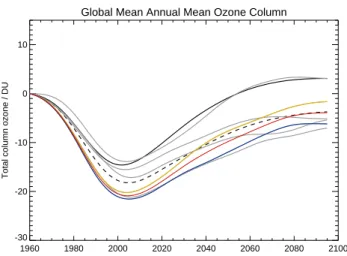
To test this procedure, it was applied to a set of six CCM simulations which assumed GHG concentrations remained fixed at their 1960 levels from 1960–2100 (note that these simulations are not used elsewhere in this study, but are ex-tensively documented in Eyring et al. (2010). This set of sim-ulations will be referred to as the fGHG simsim-ulations). Fig-ure 1 shows the smooth trend in global mean total column ozone (relative to 1960 values) of the multi-model mean for the REF-B2 simulations of the six models (solid black line) and the multi-model mean for the fGHG simulations of the six models (dashed black line). The procedure for the esti-mation of the pseudo multi-model mean trend for the fGHG scenario based on a limited number of CCM simulations is illustrated by the grey, blue and yellow lines. In each case, the grey, blue or yellow line represents an estimate of the fGHG multi-model mean calculated by adding shf (t) calcu-lated from a single CCM onto to the multi-model mean of the REF-B2 simulations. Each of the grey lines is an esti-mate of the dashed black line calculated by a simple aver-age of the six fGHG simulations. Clearly, for a single CCM, the estimate of the multi-model mean can be very different to the true multi-model mean. In the case of CCSRNIES (yellow line) and WACCM (blue line), which, along with GEOSCCM, ran SRES GHG sensitivity simulations used in the later analysis, both models somewhat overestimate the sensitivity of the global mean ozone column around the time of maximum ozone depletion, but by the end of century are close to the multi-model mean.

For the global mean and similar tests in other geographi-cal regions (not shown) when the pseudo multi-model mean is calculated from two model integrations (red line in this example) the estimate is closer to the true multi-model mean. Of course, as more and more scenario simulations are added to the average shift calculation the pseudo multi-model mean timeseries will better approximate the true multi-model mean. The example calculations here show that for two mod-els, the pseudo multi-model mean is reasonably close to the true multi-model mean (i.e. that estimated from the full en-semble of models) and generally approximates the main fea-tures of the true multi-model mean.

3.2.2 Method 2: estimating scenario uncertainty from runs of a single CCM

An alternative method for estimating scenario uncertainty is to use multiple simulations of a single CCM forced with a range of different scenarios. A set of simulations of this type is available for the RCP forcing scenarios from the CAM3.5

(7)

Global Mean Annual Mean Ozone Column 1960 1980 2000 2020 2040 2060 2080 2100 -30 -20 -10 0 10

Total column ozone / DU

Fig. 1. Multi-model mean smooth trend in ozone for six models (CCSRNIES, CMAM, MRI, SOCOL, ULAQ and WACCM) for the standard REF scenario (black solid line) and for a scenario with fixed greenhouse gas concentrations at 1960 levels (black dashed line). Grey lines show estimate of the multi-model mean trend in the fixed GHG scenario, calculated by adding the shift between the REF and fixed GHG scenario runs to the multi-model mean trend from the REF scenario for each of the six models. Estimates produced using the CCSRNIES (yellow) and WACCM (blue) models are highlighted in colour. The estimate of the multi-model mean calculated by averaging the shift in the CCSRNIES and WACCM models is shown in the red line.

30

Fig. 1. Multi-model mean smooth trend in ozone for six models

(CCSRNIES, CMAM, MRI, SOCOL, ULAQ and WACCM) for the standard REF scenario (black solid line) and for a scenario with fixed greenhouse gas concentrations at 1960 levels (black dashed line). Grey lines show estimate of the multi-model mean trend in the fixed GHG scenario, calculated by adding the shift between the REF and fixed GHG scenario runs to the multi-model mean trend from the REF scenario for each of the six models. Estimates pro-duced using the CCSRNIES (yellow) and WACCM (blue) models are highlighted in colour. The estimate of the multi-model mean calculated by averaging the shift in the CCSRNIES and WACCM models is shown in the red line.

CCM. Since three simulations of this model with different RCP scenarios are available it is trivial to calculate the time evolving scenario uncertainty by computing the standard de-viation of the ensemble of three CAM3.5 simulations. This estimate of scenario uncertainty can be compared to the es-timates derived from method 1, and together with the esti-mates of model uncertainty and internal variability from the REF ensemble to provide a breakdown of the uncertainty in ozone projection.

For the RCP scenario simulations of CAM3.5, there are significant differences in the tropospheric ozone column be-tween the runs, because tropospheric ozone precursors vary between the different scenarios. Since the focus of this study is on uncertainties in projections of stratospheric ozone, when calculating scenario uncertainty from the RCP simu-lations of CAM3.5 only the ozone column above 200 hPa is considered.

The major disadvantage of this approach is that it relies completely on an accurate simulation of the sensitivity of stratospheric ozone to each forcing scenario by the CAM3.5 model. If this model over or under estimates the sensitivity of stratospheric ozone to changes in for example GHG amounts then the estimate of scenario uncertainty will be similarly bi-ased.

4 Results

4.1 Global mean ozone

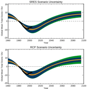
To introduce the concept of our quantification of uncertainty we first show a time series of the global and annual mean, to-tal column ozone (Fig. 2). The modelled evolution of ozone for both the past and projected future is shown (in grey), cal-culated by computing the ensemble mean of the REF and SRES simulations and is identical in both panels. Estimates of the model uncertainty and internal variability are drawn from the REF-B2 simulations, and are identical in the two panels. Shaded regions show the one standard deviation un-certainty associated with each of the three unun-certainty com-ponents. The two panels use the two alternative methods of estimating scenario uncertainty using the SRES scenario simulations (top panel) and the RCP scenario simulations (bottom panel).

Considering first the top panel, it is clear that when using the SRES scenario simulations, total uncertainty is similar throughout the 21st century, with a small reduction around the 2040s as ozone returns to its 1980 values. The relative contributions of model uncertainty (blue) and scenario un-certainty (green), however, change markedly over the course of the 21st century. For short lead times, close to peak ozone depletion, model uncertainty is large, and is likely related to the variation in stratospheric inorganic chlorine (Cly) (Eyring

et al., 2007) and related variations in chemistry, dynamics and transport between the models. By the end of the 21st century, when Clyconcentrations have returned to pre-1980

levels, model uncertainty is significantly smaller.

It is worth noting in passing that while running initial con-dition ensembles of ozone projections would help to better determine the mean smooth trend of ozone, the uncertainty in the projections related to internal atmospheric variability would remain. As described in the methods section, inter-nal variability is estimated from the model integrations them-selves and is assumed to be constant throughout the period of the runs. Examination of the time-evolving residuals for both the global ozone and other geographical regions revealed that in general there are no significant changes in the internal vari-ability estimated from the 13 models in the REF-B2 ensem-ble. For global mean values, there are variations of around 0.1 DU in the one standard deviation estimate of internal vari-ability, with a small trend toward smaller internal variability over the course of the 21st century. For the polar regions, there are slightly larger uncertainties in the estimate of in-ternal variability (as expected given the smaller averaging area and shorter averaging period) with larger variations over Antarctica of around 2–3 DU and a peak in internal variabil-ity near to the period of maximum ozone depletion. We con-sider these variations to be small enough that an assumption of constant internal variability is a valid first approximation for the analysis conducted in this study. It is also impor-tant to note that since internal variability is estimated from

(8)

SRES Scenario Uncertainty 1960 1980 2000 2020 2040 2060 2080 2100 Year -20 -10 0 10 20

Global Mean Total Ozone / DU

RCP Scenario Uncertainty 1960 1980 2000 2020 2040 2060 2080 2100 Year -20 -10 0 10 20

Global Mean Total Ozone / DU

Fig. 2. Changes in annual-mean, global-mean, total-column ozone amounts relative to 1980

values. Black dots indicate observed changes from the NIWA combined and patched ozone column dataset. The grey solid line shows the multi-model, multi-scenario mean. Coloured wedges indicate the cumulative uncertainty in this projection associated with one standard-deviation estimates of internal variability (orange), model uncertainty (blue) and scenario un-certainty (green). The top panel shows calculations of scenario unun-certainty using four model simulations run with SRES scenarios. The bottom panel shows calculations of scenario uncer-tainty using three integrations of CAM3.5 run with RCP scenarios.

31

Fig. 2. Changes in annual-mean, global-mean, total-column ozone

amounts relative to 1980 values. Black dots indicate observed

changes from the NIWA combined and patched ozone column dataset. The grey solid line shows the multi-model, multi-scenario mean. Coloured wedges indicate the cumulative uncertainty in this projection associated with one standard-deviation estimates of in-ternal variability (orange), model uncertainty (blue) and scenario uncertainty (green). The top panel shows calculations of scenario uncertainty using four model simulations run with SRES scenarios. The bottom panel shows calculations of scenario uncertainty using three integrations of CAM3.5 run with RCP scenarios.

the models themselves, it could be larger than the estimate shown here if the models under-represent tropospheric and stratospheric internal variability, but given the limited obser-vational record (black dots in Fig. 2) it is difficult to assess the magnitude of the internal variability. Additionally, if pro-jections of annual mean global mean ozone were considered, (rather than projections of decadal mean global mean ozone) internal variability would be a larger contributor to the to-tal uncertainty in ozone projections (increasing by around a factor of 2).

From the middle of the 21st century, scenario uncertainty begins to play a bigger role in determining the total uncer-tainty, as expected, since the input GHG concentrations only start to significantly diverge in the second half of the 21st century. By the end of the 21st century, when GHG concen-trations in the various scenarios have significantly diverged, their impacts on stratospheric temperatures, and hence on the rates of gas-phase ozone loss cycles and changes in strato-spheric circulation can be clearly seen by the growth of the scenario uncertainty component. Despite this growth in sce-nario uncertainty in the SRES simulations, model uncertainty

remains the largest contributor to the total uncertainty in global ozone throughout the 21st century.

In contrast to the SRES scenario simulations, scenario un-certainty is a larger component of the total unun-certainty in the RCP scenario simulations. Given the larger spread in GHG amounts in the RCP simulation this would have been expected a priori. However, scenario uncertainty from the RCP scenarios begins to dominate uncertainty in global mean ozone only by the later third of the 21st century, and not be-fore global mean ozone has returned to its pre-1980 values. The enhanced scenario uncertainty also means that the total uncertainty in projections of total ozone is larger, but only by a factor of around 20% by the end of the 21st century when compared to the total uncertainty computed using SRES sce-nario uncertainty. It is important to again point out that the assessment of the RCP scenarios is based on the low-top CAM3.5 model only. Studies using these scenarios would be useful to assess the robustness of the result.

One benefit of dividing ozone projection uncertainty into model, scenario and internal variability components is that it gives an indication of the benefit in narrowing projection un-certainty that can be made by improving CCMs and where this improvement is likely to be most beneficial. In dis-cussing these improvements, it is assumed that by improv-ing CCMs, model uncertainty will be reduced, whilst sce-nario uncertainty will remain constant, since scesce-nario uncer-tainty is primarily related to future global development paths. Under this assumption, results for both the SRES and RCP scenario cases suggest that it should be possible to narrow uncertainty in ozone projections throughout the 21st century by reducing model uncertainty. Projections of the increase in global column ozone amounts above 1980 values by the end of the 21st century are more dependent upon the con-centrations of GHGs at this time. In general, scenarios with larger emissions of GHGs (SRESA2, RCP8.5) tend to pro-duce larger amounts of ozone at the end of the 21st century.

4.2 Uncertainty in ozone projections in different geographical regions

A similar quantification of uncertainty can be performed for total column ozone projections for various geographical re-gions and seasons to highlight the different behaviour of ozone and the importance of different physical processes in determining future ozone behaviour. In this analysis we con-sider similar regions to WMO assessments of future ozone listed in Table 2.

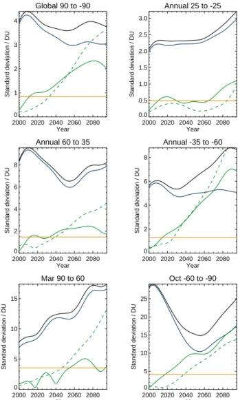
Uncertainty in the three different components, along with the total uncertainty is displayed in units of one standard de-viation in Fig. 3. Broadly, the same behaviour as identified in the global ozone concentrations is seen, with total uncer-tainty (black lines) roughly constant throughout the 21st cen-tury when SRES simulations are used to assign scenario un-certainty. In general, there is also good agreement in both the estimated magnitude and temporal evolution of scenario

(9)

Table 2. Geographical regions considered in the analysis.

Region Area Season

Global Mean 90◦S–90◦N Annual

Tropics 25◦S–25◦N Annual

NH Mid-latitudes 35◦N–60◦N Annual

SH Mid-latitudes 60◦S–35◦S Annual

NH Polar Cap (Arctic) 60◦N–90◦N March

SH Polar Cap (Antarctic) 90◦S–60◦S October

uncertainty between 2000 and 2050 for the two independent estimates derived from the SRES (solid green lines) and RCP (dashed green lines) scenarios. After 205, in the global mean, NH mid-latitudes and Arctic regions, scenario uncertainty in the RCP scenarios increases more rapidly than in the SRES scenarios. Note that scenario uncertainty for both the SRES and RCP estimates is close to but not equal to zero in the year 2000. At this time in both the SRES and RCP scenarios there is almost no difference in GHG concentrations, sug-gesting that the small offset here is related to uncertainties in the estimation of the S(t)2_term.

In most regions, when SRES scenarios are considered, model uncertainty remains the dominant term in the uncer-tainty budget throughout the 21st century. When scenario uncertainty is calculated from the RCP scenarios, in some regions (Global mean, SH mid-latitudes) total uncertainty undergoes a transition from model dominated uncertainty to scenario dominated uncertainty at some time in the last third of the century. However, there are significant differences to this behaviour in different regions.

In the tropics, model uncertainty remains a large contribu-tor to the uncertainty throughout the 21st century and grows slightly from 2000 to 2100. SRES and RCP scenario uncer-tainty remains small throughout the 21st century. The evolu-tion of tropical column ozone is determined by the balance between increases in upper stratospheric ozone due to strato-spheric cooling and decreases in lower stratostrato-spheric ozone due to increases in the strength of the Brewer-Dobson circu-lation. Comparison of vertically resolved ozone changes (not shown) indicate that a robust feature in the GHG sensitiv-ity simulations is that, in the tropical upper stratosphere, the lower GHG scenarios generally result in lower ozone (due to smaller GHG-induced ozone increases), whereas in the lower stratosphere the lower GHG scenarios result in higher ozone (due to less tropical upwelling that advects ozone-poor air from the troposphere).

All CCMs also consistently predict an increase of tropical upwelling with increasing GHGs, but the significant varia-tion in Brewer-Dobson circulavaria-tion strength that was found amongst the CCMVal2 models (Chapter 4, SPARC CCM-Val, 2010, see also Fig. 7 of Eyring et al., 2010) plays a significant role in determining the large model uncertainty and its growth with time (since models with larger

tropi-Global 90 to -90 2000 2020 2040 2060 2080 Year 0 1 2 3 4 Standard deviation / DU Annual 25 to -25 2000 2020 2040 2060 2080 Year 0.0 0.5 1.0 1.5 2.0 2.5 3.0 Standard deviation / DU Annual 60 to 35 2000 2020 2040 2060 2080 Year 0 2 4 6 8 Standard deviation / DU Annual -35 to -60 2000 2020 2040 2060 2080 Year 0 2 4 6 8 Standard deviation / DU Mar 90 to 60 2000 2020 2040 2060 2080 Year 0 5 10 15 Standard deviation / DU Oct -60 to -90 2000 2020 2040 2060 2080 Year 0 5 10 15 20 25 Standard deviation / DU

Fig. 3. Uncertainty in the predicted total-column ozone amounts, relative to 1980 values, es-timated for different geographic regions (global, annual mean - top left, tropical annual mean - top right, NH mid-latitudes, annual - middle let, SH mid-latitudes, annual - middle right, NH polar cap, March - bottom left, SH polar cap bottom right). Uncertainty is expressed as the one standard deviation estimate for interannual variability (orange), model uncertainty (blue) and scenario uncertainty (green) and the total (black). Solid green lines show calculations of scenario uncertainty using four model integrations run with SRES scenarios. Dashed green lines show calculations of scenario uncertainty using three integrations of CAM3.5 run with RCP scenarios.

Fig. 3. Uncertainty in the predicted total-column ozone amounts,

relative to 1980 values, estimated for different geographic regions (global, annual mean – top left, tropical annual mean – top right, NH latitudes, annual – middle let, SH latitudes, annual – mid-dle right, NH polar cap, March – bottom left, SH polar cap bottom right). Uncertainty is expressed as the one standard deviation esti-mate for interannual variability (orange), model uncertainty (blue) and scenario uncertainty (green) and the total (black). Solid green lines show calculations of scenario uncertainty using four model in-tegrations run with SRES scenarios. Dashed green lines show calcu-lations of scenario uncertainty using three integrations of CAM3.5 run with RCP scenarios.

cal upwelling mass flux also tend to exhibit larger trends in mass flux over the 21st century (Chapter 4, SPARC CCM-Val, 2010)). Consequently, uncertainty in projections of trop-ical ozone is likely to significantly benefit from improve-ments in CCMs transport schemes as well as improveimprove-ments in the underlying dynamics of the General Circulation Mod-els (GCMs).

(10)

Over the polar regions, while internal variability plays a larger role than in the other geographical regions, model un-certainty remains the dominant term in the total unun-certainty for most of the 21st century. The role of internal variabil-ity is most prominent over the Arctic, where it is larger than scenario uncertainty till around 2050 for both scenario un-certainty estimates.

Model uncertainty over the Antarctic reduces markedly over the first half of the 21st century and reaches a minimum in 2050 before increasing toward the end of the century. One hypothesis for this behaviour is that most of the model uncer-tainty in the first half of the 21st century is related to the rep-resentation of heterogeneous chemical ozone depletion and becomes smaller as ODS concentrations decrease. The in-crease in model uncertainty in the Antarctic from 2050 to the end of the century is similar to the consistent increase in model uncertainty in the Arctic throughout the 21st cen-tury. One hypothesis for this growth of model uncertainty is that because the response to GHG changes has a wide spread between models, model uncertainty increases linearly with time as the spread in the changes becomes larger (but the response to GHG changes evolves consistently within each model). Further, process-based studies would be required to test these hypotheses.

While scenario uncertainty for both SRES and RCP sce-narios grows over the 21st century for both polar cap regions there is a larger difference between the estimation of this un-certainty from the SRES and RCP scenarios over the Arctic than over the Antarctic. For the Antarctic, scenario uncer-tainty is broadly similar for the SRES and RCP scenario sets, and has similar size to model and internal variability from around 2050. For the Arctic, RCP scenario uncertainty grows much more strongly than SRES scenario uncertainty over the 21st century, but is smaller than model uncertainty in both cases. For regions like the Arctic where model uncertainty is large, scenario uncertainty estimates likely have larger error bars because they rely on runs of a small number of CCMs which may have different responses to GHG changes.

Over the polar caps, these results suggests that there are very different potential benefits to improving CCMs. Over the Arctic, reducing model uncertainty could have a signifi-cant impact on the total uncertainty throughout the 21st cen-tury, since this term is large and increases substantially from 2000 to 2100. Over the Antarctic, the reduction in model uncertainty and the growth of scenario uncertainty means that the impact of a reduction in model uncertainty would be largest for the first two-thirds of the 21st century. The Antarctic also has a minimum in total uncertainty around 2050, similar to that seen in projections of global mean and regional surface temperature (Hawkins and Sutton, 2009).

4.3 Signal-to-noise ratio of ozone projections

As in Hawkins and Sutton (2009, 2010), the uncertainty es-timates shown above can be used to determine other

impor-tant properties of the ozone projections, such as the signal-to-noise ratio (S/N),

S/N =multi − model mean ozone change total uncertainty .

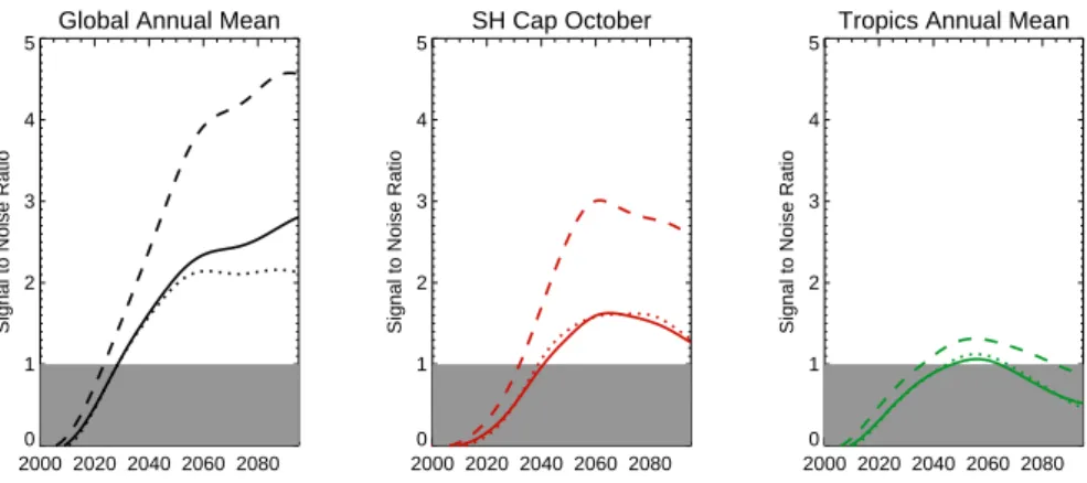
Where S/N exceeds one, there is a detectable change in ozone predicted by the multi-model ensemble. For near-surface temperature, Hawkins and Sutton (2009) used S/N to quan-tify periods in which the potential information content of projections was greatest. In the case of stratospheric ozone projections, we consider the change in total column ozone from 2000, the year chosen as the start of our projection pe-riod and close to the minimum in ozone column amounts. Where S/N is greater than one, this suggests that the model ensemble predicts a detectable change from 2000 values. Figure 4 shows estimates of S/N for three of the geographi-cal regions described above, with SRES scenario uncertainty (solid), RCP scenario uncertainty (dotted) and without sce-nario uncertainty (dashed) included. The S/N is estimated with and without scenario uncertainty to allow a more direct comparison with many previous studies and assessments of future ozone amounts which have tended to focus on a single GHG scenario.

It is clear from Fig. 4 that, in all three regions, including either SRES or RCP scenario uncertainty significantly de-grades the ability of the model ensemble to predict changes in column ozone amounts, as expected. The date at which projections in all regions have S/N greater than one, and hence predict a detectable change in column ozone, is de-layed by around 5 years in the global mean and 10 years for the Antarctic and tropical cases. In the global mean case, if the RCP scenario uncertainty is used instead of the SRES scenario uncertainty, S/N remains approximately constant af-ter 2050, as scenario uncertainty becomes larger than model uncertainty. When scenario uncertainty is not considered, the signal-to-noise ratio continues to grow, indicating increased confidence in projections. This is an alternative way of show-ing that CCM improvements would likely benefit projections of column ozone by the largest amount in the early part of the 21st century, up to the date of ozone return to 1980 values.

Over the Antarctic, although the signal of ozone increases from 2000 values is larger than the global mean signal, the signal to noise ratio is smaller because of the greater total uncertainty. The difference between the estimates of S/N us-ing SRES and RCP scenario uncertainty estimates are very small.

In the tropical region, the evolution of S/N is somewhat different, with a noticeable peak in mid-century (where the difference between current and future column amounts is greatest) before a decline in the second half of the century. The difference between S/N with and without scenario un-certainty is less pronounced for the tropics, with only a small reduction in S/N when either SRES or RCP scenario uncer-tainty is included. It should also be noted, however, that the

(11)

size of S/N in the tropics is smaller than for either the global mean or the Antarctic.

4.4 Uncertainty in ozone return date

Finally, we consider how different sources of uncertainty in-fluence the calculation of the return date for total-column ozone to its 1980 value. To do this, a different calculation procedure is required.

It is assumed that the calculation of return date will be post-hoc (i.e. based on the transition of a smooth estimate of the long-term trend in ozone across the zero line). It is there-fore simple to estimate the uncertainty in return date due to model uncertainty (by calculating the variance of return dates across the model ensemble) and due to scenario uncertainty (by calculating the variance of return dates across the REF-B2 and pseudo multi-model mean estimates for each scenario using method 1 and across the RCP ensemble using method 2). To calculate the contribution of internal variability to un-certainty in return date, a Monte-Carlo approach is adopted. For each model, the residuals from the smooth model trend are randomly permuted and added back to the model trend to give an alternative evolution of column ozone. By fitting a smooth trend to this new synthetic data and estimating the return date, and then repeating this procedure 10 000 times, an estimate of the uncertainty in return date due to internal variability in each model can be made. The mean of the in-ternal variability uncertainty for the 13 models in the REF-B2 ensemble is used to estimate the overall uncertainty due to internal variability. Note that this estimate may be slightly smaller than the real contribution of internal variability to the uncertainty in return date, since we neglect to preserve the decadal variability present in the noise term when we per-mute the residuals using this method.

Fractional standard deviation in return date for Arctic, Antarctic and global ozone is shown in Fig. 5 as bars which add up to 1 (or 100% of the total standard deviation). As in previous calculations, it is clear that a substantial part of the uncertainty in return date is associated with model un-certainty. This conclusion is not dependent upon the source of the scenario uncertainty estimate, although scenario un-certainty in return date is greater for the SRES simulations over the Antarctic and greater for the RCP simulations over the Arctic. Over these three key averaging regions, the maximum contribution to the fractional standard deviation in ozone return date is around 45% for the Antarctic using SRES scenario uncertainty and the minimum contribution is around 10% for the Antarctic using RCP scenario uncertainty estimates. There is therefore strong potential to improve es-timates of the return date for ozone in these regions by con-tinued CCM development.

5 Conclusions

In this study, an attempt to quantify the uncertainty in fu-ture projections of total ozone column amounts has been made. In particular, a method introduced and tested for the CMIP3 models has been adapted and developed for models run as part of the Chemistry-Climate Model Validation ac-tivity (CCMVal2). Projection uncertainty has been divided into three components representing model uncertainty, sce-nario uncertainty and uncertainty due to internal variability of the system. Scenario uncertainty has been estimated using two different methods which used scenario simulations from both SRES and RCP future emission scenarios.

When considering scenario uncertainty in the SRES sce-narios, total uncertainty in ozone projections is roughly con-stant throughout the 21st century and is dominated by model uncertainty. Although scenario uncertainty in the SRES sce-nario simulations grows throughout the 21st century, for most geographical regions and seasons it remains smaller than model uncertainty.

When considering scenario uncertainty in the RCP scenar-ios, total uncertainty grows slightly throughout the 21st cen-tury, due to a larger growth in scenario uncertainty than for the SRES simulations. There is an important transition be-tween model uncertainty and scenario uncertainty for some regions (notably the global mean ozone and ozone in the SH mid-latitudes) with scenario uncertainty dominating projec-tions by the last third of the 21st century. This has important consequences for the ability of models to predict significant changes to ozone column amounts, which is degraded by sce-nario uncertainty during this period.

In general, the consistency of the two independent esti-mates of scenario uncertainty for most diagnostics lends con-fidence in these estimates. However, the application of the scenario uncertainty should proceed with some caution. The GHG scenarios used by the models are designed to provide an estimate of the potential range of future emissions based on vastly different global economic and technological devel-opment. The scenarios are not equally likely, do not take into account all possible futures and should not be taken to indicate an upper bound on the range of potential future sions. The newer RCP scenarios have a larger spread in emis-sions of GHGs compared to the SRES scenarios used, partly due to the inclusion of the very low GHG emission scenario (RCP2.6) which represents a future scenario with peak ra-diative forcing around 2050. This scenario does not have an obvious equivalent in the SRES scenarios considered.

An additional source of uncertainty in projections of ozone which we did not consider in this study are the mean state bi-ases between CCMs. In all cbi-ases, CCM time series of ozone were corrected to their 1980 values as is customary in the CCM community. As shown in, for example, Chapter 9 of the CCMVal report, in many regions models have large basic state biases in the total ozone column. If these uncertainties were taken into account they would likely further increase

(12)

Global Annual Mean 2000 2020 2040 2060 2080 0 1 2 3 4 5

Signal to Noise Ratio

SH Cap October 2000 2020 2040 2060 2080 0 1 2 3 4 5

Tropics Annual Mean

2000 2020 2040 2060 2080 0 1 2 3 4 5

Fig. 4. Estimated signal-to-noise ratio (S/N, see text for details) of the change in total-ozone

column amounts relative to the multi-model mean amount in 2000. Solid lines show estimates which include model uncertainty, internal variability and scenario uncertainty from four model integrations run with SRES scenarios. Dotted lines show estimates which include model un-certainty, internal variability and scenario uncertainty from three model integrations of CAM3.5 run with RCP scenarios. Dashed lines show estimates which exclude scenario uncertainty. Different coloured lines indicate averages over different geographical regions and seasons. Black lines show the global and annual average, red lines show the springtime SH polar cap (60-90◦_{S, October) and the green lines show the tropical region (25}◦_N-25◦_{S), annual average).} Grey shading highlights the region with S/N less than 1.

33

Fig. 4. Estimated signal-to-noise ratio (S/N, see text for details) of the change in total-ozone column amounts relative to the multi-model

mean amount in 2000. Solid lines show estimates which include model uncertainty, internal variability and scenario uncertainty from four model integrations run with SRES scenarios. Dotted lines show estimates which include model uncertainty, internal variability and scenario uncertainty from three model integrations of CAM3.5 run with RCP scenarios. Dashed lines show estimates which exclude scenario uncertainty. Different coloured lines indicate averages over different geographical regions and seasons. Black lines show the global and

annual average, red lines show the springtime SH polar cap (60–90◦S, October) and the green lines show the tropical region (25◦N–25◦S),

annual average). Grey shading highlights the region with S/N less than 1.

the relative contribution of model uncertainty to the total un-certainty estimates we have derived.

The quantification of uncertainty derived in our study also provides some insight into the ability of the Chemistry-Climate modelling community to refine projections of future ozone amounts by the continued development and improve-ment of CCMs. The results of our analysis suggest that this work would be beneficial for projections of ozone amounts in the first half of the 21st century in most regions and particu-larly in the determination of dates of return of ozone amounts to pre-1980 values (a key metric for ozone defined by the 2006 WMO/UNEP ozone assessment). In future, similar methods could be used to quantify the uncertainty in pro-jections of other parameters of the stratospheric climate sys-tem in order to attribute the scenario uncertainty to differ-ent physical processes. It is also important to note, however, that the relationship between spread and skill for geophysical models is far from trivial. While it is reasonable to wish to reduce overall uncertainty in projections of future ozone, it does not necessarily follow that narrowing the uncertainty in these projections will also improve their skill.

The quantification of uncertainty in ozone projections in this study is far from ideal and is sensitive to the assumptions and models used, particularly in constructing estimates of scenario uncertainty. It is hoped that the results will provide guidance to the chemistry-climate community on the benefits that running large multi-scenario ensembles of CCMs would provide. It is clear from our initial analysis that the benefits in fully quantifying and exploring the projection uncertainty from running multi-scenario ensemble simulations vary sub-stantially between different geographical regions, seasons and time-periods. We re-iterate that an ideal ensemble of simulations for the quantification of uncertainty introduced

NH Cap SH Cap Global

0.0 0.2 0.4 0.6 0.8 1.0

Fractional Standard Deviation

Fig. 5. Estimates of the fractional uncertainty in the date of return to 1980 values of total-column

ozone amounts due to different sources of uncertainty, for three different geographical regions and seasons. The coloured areas indicate the fractional contribution of that type of uncertainty to overall uncertainty in the date of ozone return date (orange - internal variability, blue - model uncertainty, green - scenario uncertainty). Bars are shown for the northern polar cap during

spring (60-90◦_{N, March) for the southern polar cap during spring (60-90}◦_{S, October) and for}

the global and annual. Left-side bars show calculations of scenario uncertainty using four model integrations run with SRES scenarios. Right-side bars shows calculations of scenario uncertainty using three integrations of CAM3.5 run with RCP scenarios.

34

Fig. 5. Estimates of the fractional uncertainty in the date of return to

1980 values of total-column ozone amounts due to different sources of uncertainty, for three different geographical regions and seasons. The coloured areas indicate the fractional contribution of that type of uncertainty to overall uncertainty in the date of ozone return date (orange – internal variability, blue – model uncertainty, green – sce-nario uncertainty). Bars are shown for the northern polar cap during

spring (60–90◦N, March) for the southern polar cap during spring

(60–90◦S, October) and for the global and annual. Left-side bars

show calculations of scenario uncertainty using four model integra-tions run with SRES scenarios. Right-side bars shows calculaintegra-tions of scenario uncertainty using three integrations of CAM3.5 run with RCP scenarios.

here would require a large ensemble of models to all run at least three different GHG scenarios.

(13)

Acknowledgements. This work was carried out as part of the ongoing CCMVal2 project. We acknowledge the support of Mar-tine Michou and Hubert Teyssedre (CNRM-ACM, Meteo-France) and John Austin (AMTRAC3, GFDL) for supplying model data from the REF-B2 runs along with the support of the many scientists who contributed analysis and data to the SPARC CCMVal report which allowed us to make rapid progress on understanding the

different model simulations. We also acknowledge the British

Atmospheric Data Centre for providing the data archive for the simulations. CCSRNIES research was supported by the Global Environmental Research Fund of the Ministry of the Environment of Japan (A-071) and the simulations were completed with the super computer at CGER, NIES. The MRI simulation was made with the supercomputer at the National Institute for Environmental Studies, Japan.

Edited by: W. Lahoz

References

Akiyoshi, H., Zhou, L. B., Yamashita, Y., Sakamoto, K., Yoshiki, M., Nagashima, T., Takahashi, M., Kurokawa, J., Takigawa,

M., and Imamura, T.: A CCM simulation of the breakup

of the Antarctic polar vortex in the years 1980-2004 un-der the CCMVal scenarios, J. Geophys. Res., 114, D03103, doi:10.1029/2007JD009261, 2009.

Austin, J. and Wilson, R. J.: Sensitivity of polar ozone to sea surface temperatures and chemistry, J. Geophys. Res., in press, 2010. Barnett, J. J., Houghton, J. T., and Pyle, J. A.: The temperature

dependence of the ozone concentration near the stratopause, Q. J. Roy. Meteor. Soc., 101, 245–257, 1974.

Butchart, N., Scaife, A. A., Bourqui, M., de Grandpr´e, J., Hare, S. H. E., Kettleborough, J., Langematz, U., Manzini, E., Sassi, F., Shibata, K., Shindell, D., and Sigmond, M.: Simulations of an-thropogenic change in the strength of the Brewer-Dobson circu-lation, Climate Dynam., 27, 727–741, doi:10.1007/s00382-006-0162-4, 2006.

Chipperfield, M. P. and Feng, W.: Comment on: Stratospheric Ozone Depletion at northern mid-latitudes in the 21st century: The importance of future concentrations of greenhouse gases nitrous oxide and methane, Geophys. Res. Lett., 30, 1389, doi:10.1029/2002GL016353, 2003.

Clarke, L., Edmonds, J., Jacoby, H., Pitcher, H., Reilly, J., and Richels, R.: Scenarios of Greenhouse Gas Emissions and Atmo-spheric Concentrations, Sub-report 2.1A of Synthesis and As-sessment Product 2.1 by the U.S. Climate Change Science Pro-gram and the Subcommittee on Global Change Research. De-partment of Energy, Office of Biological & Environmental Re-search, Washington, 7 DC, USA, 154 pp., 2007.

de Grandpr´e, J., Beagley, S. R., Fomichev, V. I., Griffioen, E., Mc-Connell, J. C., Medvedev, A. S., and Shepherd, T. G.: Ozone climatology using interactive chemistry: Results from the Cana-dian Middle Atmosphere Model, J. Geophys. Res., 105, 26475– 26491, 2000.

D´equ´e, M.: Frequency of precipitation and temperature extremes over France in an anthropogenic scenario: model results and sta-tistical correction according to observed values, Global Planet. Change, 57, 16–26, 2007.

Egorova, T., Rozanov, E., Zubov, V., Manzini, E., Schmutz, W., and Peter, T.: Chemistry-climate model SOCOL: a validation of the present-day climatology, Atmos. Chem. Phys., 5, 1557–1576, doi:10.5194/acp-5-1557-2005, 2005.

Eyring, V., Butchart, N., Waugh, D. W., Akiyoshi, H., Austin, J., Bekki, S., Bodeker, G. E., Boville, B. A., Br¨uhl, C., Chipper-field, M. P., Cordero, E., Dameris, M., Deushi, M., Fioletov, V. E., Frith, S. M., Garcia, R. R., Gettelman, A., Giorgetta, M. A., Grewe, V., Jourdain, L., Kinnison, D. E., Mancini, E., Manzini, E., Marchand, M., Marsh, D. R., Nagashima, T., Newman,P. A., Nielsen, J. E., Pawson, S., Pitari, G., Plummer, D. A., Rozanov, E., Schraner, M., Shepherd, T. G., Shibata, K., Stolarski, R. S., Struthers, H., Tian, W., and Yoshiki, M.: Assessment of tem-perature, trace species and ozone in chemistry-climate model simulations of the recent past, J. Geophys. Res., 111, D22308, doi:10.1029/2006JD007327, 2006.

Eyring, V., Waugh, D. W., Bodeker, G. E., Cordero, E., Akiyoshi, H., Austin, J., Beagley, S. R., Boville, B., Braesicke, P., Br¨uhl, C., Butchart, N., Chipperfield, M. P., Dameris, M., Deckert, R., Deushi, M., Frith, S. M., Garcia, R. R., Gettelman, A., Giorgetta, M., Kinnison, D. E., Mancini, E., Manzini, E., Marsh, D. R., Matthes, S., Nagashima, T., Newman, P. A., Nielsen, J. E., Paw-son, S., Pitari, G., Plummer, D. A., Rozanov, E., Schraner, M., Scinocca, J. F., Semeniuk, K., Shepherd, T. G., Shibata, K., Steil, B., Stolarski, R., Tian, W., and Yoshiki, M.: Multimodel projec-tions of stratospheric ozone in the 21st century, J. Geophys. Res., 112, D16303, doi:10.1029/2006JD008332, 2007.

Eyring, V., Cionni, I., Bodeker, G. E., Charlton-Perez, A. J., Kinni-son, D. E., Scinocca, J. F., Waugh, D. W., Akiyoshi, H., Bekki, S., Chipperfield, M. P., Dameris, M., Dhomse, S., Frith, S. M., Garny, H., Gettelman, A., Kubin, A., Langematz, U., Mancini, E., Marchand, M., Nakamura, T., Oman, L. D., Pawson, S., Pitari, G., Plummer, D. A., Rozanov, E., Shepherd, T. G., Shi-bata, K., Tian, W., Braesicke, P., Hardiman, S. C., Lamarque, J. F., Morgenstern, O., Pyle, J. A., Smale, D., and Yamashita, Y.: Multi-model assessment of stratospheric ozone return dates and ozone recovery in CCMVal-2 models, Atmos. Chem. Phys., 10, 9451–9472, doi:10.5194/acp-10-9451-2010, 2010.

Garcia, R. R., Marsh, D. R., Kinnison, D. E., Boville, B. A., and Sassi, F.: Simulation of secular trends in the mid-dle atmosphere, 1950–2003, J. Geophys. Res., 112, D09301, doi:10.1029/2006JD007485, 2007.

Haigh, J. D. and Pyle, J. A.: Ozone perturbation experiments in a two-dimensional circulation model, Q. J. Roy. Meteorol. Soc., 108, 551–574, 1982.

Hawkins, E. and Sutton, R.: The potential to narrow uncertainty in regional climate predictions, B. Am. Meteor. Soc., 90, 1095, doi:10.1175/2009BAMS2607.1, 2009.

Hawkins, E. and Sutton, R.: The potential to narrow uncertainty in projections of regional precipitation change, Clim. Dynam., doi:10.1007/s00382-010-0810-6, in press, 2010.

Jonsson, A. I., Fomichev, V. I., and Shepherd, T. G.: The effect

of nonlinearity in CO₂heating rates on the attribution of

strato-spheric ozone and temperature changes, Atmos. Chem. Phys., 9, 8447–8452, doi:10.5194/acp-9-8447-2009, 2009.

Jourdain, L., Bekki, S., Lott, F., and Lef`evre, F.: The coupled chemistry-climate model LMDz-REPROBUS: description and evaluation of a transient simulation of the period 1980–1999, Ann. Geophys., 26, 1391–1413,

(14)

doi:10.5194/angeo-26-1391-2008, 2008.

Lamarque, J.-F., Kinnison, D. E., Hess, P. G., and Vitt, F. M.: Sim-ulated lower stratospheric trends between 1970 and 2005: Iden-tifying the role of climate and composition changes, J. Geophys. Res., 113, D12301, doi:10.1029/2007JD009277, 2008.

Lamarque, J.-F., Bond, T. C., Eyring, V., Granier, C., Heil, A., Klimont, Z., Lee, D., Liousse, C., Mieville, A., Owen, B., Schultz, M. G., Shindell, D., Smith, S. J., Stehfest, E., Van Aardenne, J., Cooper, O. R., Kainuma, M., Mahowald, N., Mc-Connell, J. R., Naik, V., Riahi, K., and van Vuuren, D. P.: His-torical (1850–2000) gridded anthropogenic and biomass burning emissions of reactive gases and aerosols: methodology and ap-plication, Atmos. Chem. Phys., 10, 7017–7039, doi:10.5194/acp-10-7017-2010, 2010.

Meehl, G. A. and Hibbard, K. A. A Strategy for Climate Change Stabilization Experiments with AOGCMs and ESMs (2007) WCRP Informal Report No. 3/2007, ICPO Publication No. 112, IGBP Report No. 57, World Climate Research Programme, Geneva

Moss, T., Babiker, M., Brinkman, S., Calvo, E., Carter, T., Ed-monds, J., Elgizouli, I., Emori, S., Erda, L., Hibbard, K., Jones, R., Kainuma, M., Kelleher, J., Lamarque, J.-F., Manning, M., Matthews, B., Meehl, G., Meyer, L., Mitchell, J., Nakic’enovic’, N., O’Neill, B., Pichs, T., Riahi, K., Rose, S., Runci, P., Stouf-fer, R., van Vuuren, D., Weyant, J., Wilbanks, T., van Ypersele, J. P., and Zurek, M.: Towards New Scenarios for Analysis of Emissions, Climate Change, Impacts, and Response Strategies., Intergovernmental Panel on Climate Change, Geneva, 132 pp., available at: http://www.aimes.ucar.edu/docs/, 2008.

Morgenstern, O., Braesicke, P., Hurwitz, M. M., O’Connor, F. M., Bushell, A. C., Johnson, C. E., and Pyle, J. A.: The World Avoided by the Montreal Protocol, Geophys. Res. Lett., 35, L16811, doi:10.1029/2008GL034590, 2008.

Morgenstern, O., Braesicke, P., O’Connor, F. M., Bushell, A. C., Johnson, C. E., Osprey, S. M., and Pyle, J. A.: Evaluation of the new UKCA climate-composition model. Part 1: The strato-sphere, Geosci. Model Dev., 1, 43–57, 2009.

Morgenstern, O., Giorgetta, M. A., Shibata, K., Eyring V., Waugh, D. W., Shepherd, T. G., Akiyoshi, H., Austin, J., Baumgaertner, A. J. G., Bekki, S., Braesicke, P., Br¨uhl, C., Chipperfield, M. P., Cugnet, D., Dameris, M., Dhomse, S., Frith, S. M., Garny, H., Gettelman, A., Hardiman, S. C., Hegglin, M. I., Kinnison, D. E., Lamarque, J.-F., Mancini, E., Manzini, E., Marchand, M., Mi-chou, M., Nakamura, T., Nielsen, J. E., Pitari, G., Plummer, D. A., Rozanov, E., Scinocca, J. F., Smale, D., Strahan, S., Teysse-dre, H., Toohey, M., Tian, W., and Yamashita, Y.: Review of present-generation stratospheric chemistry-climate models and associated external forcings, J. Geophys. Res., in press, 2010. Nakicenovic, N., Alcamo, J., Davis, G., de Vries, B., Fenhann, J.,

Gaffin, S., Gregory, K., Grbler, A., Jung, T. Y., Kram, T., Le-bre La Rovere, E., Michaelis, L., Mori, S., Morita, T., Pepper, W., Pitcher, H., Price, L., Riahi, K., Roehrl, A., Rogner, H.-H., Sankovski, A., Schlesinger, M., Shukla, P., Smith, S., Swart, R., van Rooijen, S., Victor, N., and Dadi, Z., IPCC Special Report on Emissions Scenarios, Cambridge University Press, 2000. Oman, L., Waugh, D. W., Kawa, S. R., Stolarski, R. S., Douglass,

A. R., and Newman, P. A.: Mechanisms and feedbacks causing changes in upper stratospheric ozone in the 21st century, J. Geo-phys. Res., in press, 2010.

Oman, L. D., Plummer, D., Waugh, D. W., Austin, J., Scinocca, J., Douglass, A. R., Salawitch, R. J., Akiyoshi, H., Bekki, S., Braesicke, P., Butchart, N., Chipperfield, M., Dhomse, S., Eyring, V., Frith, S., Garcia, R. R., Gettelman, A., Hardiman, S. C., Kinnison, D., Lamarque, J. F., Mancini, E., Marchand, M., Michou, M., Morgenstern, O., Pawson, S., Pitari, G., Peter, T., Pyle, J., Rozanov, E., Shepherd, T. G., Shibata, K., Stolarski, R., Teyssedre, H., and Tian,W.: Multi-model assessment of the factors driving the ozone evolution over the 21st century, J. Geo-phys. Res., submitted, 2010.

Pawson, S., Stolarski, R. S., Douglass, A. R., Newman, P. A., Nielsen, J. E., Frith, S. M., and Gupta, M. L.: Goddard Earth Ob-serving System chemistry-climate model simulations of strato-spheric ozone-temperature coupling between 1950 and 2005, J. Geophys. Res., 113, D12103, doi:10.1029/2007JD009511, 2008. Pitari, G., Mancini, E., Rizi, V., and Shindell, D. T.: Impact of Future Climate and Emission Changes on Stratospheric Aerosols and Ozone, J. Atmos. Sci., 59, 414–440, 2002.

Portmann, R. W. and Solomon, S.: Indirect radiative forcing of the ozone layer during the 21st century, Geophys Res. Lett., 34, L02813, doi:10.1029/2006GL028252, 2007.

Randeniya, L. K., Vohralik, P. F., and Plumb, I. C.: Stratospheric ozone depletion at northern mid latitudes in the 21st century: The importance of future concentrations of greenhouse gases nitrous oxide and methane, Geophys. Res. Lett., 29(4), 1051, doi:10.1029/2001GL014295, 2002.

Ravishankara, A. R., Daniel, J. S., and Portmann, R. W.: Nitrous Oxide (N2O): The Dominant Ozone Depleting Substance Emit-ted in the 21st Century, Science, 326(123), 682–125, 2009.

Riahi, K., Gruebler, A., and Nakicenovic, N.: Scenarios of

long-term socio-economic and environmental development un-der climate stabilization, Technological Forecasting and Social Change, 74(7), 887–935, 2007.

Rosenfield, J. E., Douglass, A. R., and Considine, D. B.: The im-pact of increasing carbon dioxide on ozone recovery, J. Geophys. Res., 107(D6), 4049, doi:10.1029/2001JD000824, 2002. Schraner, M., Rozanov, E., Schnadt Poberaj, C., Kenzelmann, P.,

Fischer, A. M., Zubov, V., Luo, B. P., Hoyle, C. R., Egorova, T., Fueglistaler, S., Br¨onnimann, S., Schmutz, W., and Peter, T.: Technical Note: Chemistry-climate model SOCOL: version 2.0 with improved transport and chemistry/microphysics schemes, Atmos. Chem. Phys., 8, 5957–5974, doi:10.5194/acp-8-5957-2008, 2008.

Scinocca, J. F., N. A. McFarlane, M. Scinocca, J. F., McFar-lane, N. A., Lazare, M., Li, J., and Plummer, D.: Technical Note: The CCCma third generation AGCM and its extension into the middle atmosphere, Atmos. Chem. Phys., 8, 7055–7074, doi:10.5194/acp-8-7055-2008, 2008.

Shepherd, T. G.: Dynamics, stratospheric ozone, and climate change, Atmos. Ocean, 46, 117–138, 2008.

Shibata, K. and Deushi, M.: Long-term variations and trends in the simulation of the middle atmosphere 1980–2004 by the chemistry-climate model of the Meteorological Research In-stitute, Ann. Geophys., 26, 1299–1326, doi:10.5194/angeo-26-1299-2008, 2008a.

Shibata, K. and Deushi, M.: Simulation of the stratospheric cir-culation and ozone during the recent past (1980–2004) with the MRI chemistry-climate model, CGER’s Supercomputer Mono-graph Report Vol.13, National Institute for Environmental