Middle-energy electron anisotropies in the auroral region

HAL Id: hal-00317216

https://hal.archives-ouvertes.fr/hal-00317216

Submitted on 1 Jan 2004

HAL is a multi-disciplinary open access

archive for the deposit and dissemination of

sci-entific research documents, whether they are

pub-lished or not. The documents may come from

teaching and research institutions in France or

abroad, or from public or private research centers.

L’archive ouverte pluridisciplinaire HAL, est

destinée au dépôt et à la diffusion de documents

scientifiques de niveau recherche, publiés ou non,

émanant des établissements d’enseignement et de

recherche français ou étrangers, des laboratoires

publics ou privés.

P. Janhunen, A. Olsson, H. Laakso, A. Vaivads

To cite this version:

P. Janhunen, A. Olsson, H. Laakso, A. Vaivads. Middle-energy electron anisotropies in the auroral

region. Annales Geophysicae, European Geosciences Union, 2004, 22 (1), pp.237-249. �hal-00317216�

Annales Geophysicae (2004) 22: 237–249 © European Geosciences Union 2004

Annales

Geophysicae

Middle-energy electron anisotropies in the auroral region

P. Janhunen1, A. Olsson2, H. Laakso3, and A. Vaivads2

1_{Finnish Meteorological Institute, Geophysical Research, Helsinki, Finland} 2_{Swedish Institute of Space Physics, Uppsala Division, Uppsala, Sweden} 3_{ESTEC, Space Science Department, Noordwijk, The Netherlands}

Received: 22 January 2003 – Revised: 25 March 2003 – Accepted: 13 May 2003 – Published: 1 January 2004

Abstract. Field-aligned anisotropic electron distribution

functions of Tk> T⊥type are observed on auroral field lines

at both low and high altitudes. We show that typically the anisotropy is limited to a certain range of energies, often be-low 1 keV, although sometimes extending to slightly higher energies as well. Almost always there is simultaneously an isotropic electron distribution at higher energies. Often the anisotropies are up/down symmetrical, although cases with net upward or downward electron flow also occur. For a statistical analysis of the anisotropies we divide the energy range into low (below 100 eV), middle (100 eV–1 keV) and high (above 1 keV) energies and develop a measure of an-isotropy expressed in density units. The statistical magnetic local time and invariant latitude distribution of the middle-energy anisotropies obeys that of the average auroral oval, whereas the distributions of the low and high energy aniso-tropies are more irregular. This suggests that it is specifi-cally the middle-energy anisotropies that have something to do with auroral processes. The anisotropy magnitude de-creases monotonically with altitude, as one would expect, be-cause electrons have high mobility along the magnetic field and thus, the anisotropy properties spread rapidly to different altitudes.

Key words. Magnetospheric physics (auroral phenomena). Space plasma physics (wave-particle interactions; changed particle motion and acceleration)

1 Introduction

Field-aligned electron anisotropies have been found on auro-ral field lines at both high and low altitudes. Below 8000 km altitude, field-aligned electrons were detected by the S3-3 satellite (Sharp et al., 1980; Collin et al., 1982). Close to the equatorial plane, bidirectional anisotropies were studied us-ing IMP 6 (Hada et al., 1981), AMPTE/CCE (Klumpar et al., 1988), AMPTE/IRM (Sergeev et al., 2001) and SCATHA

Correspondence to: A. Olssen (ao@irfu.se)

(Richardson et al., 1981). Also geostationary satellites (cor-responding to invariant latitude of 67◦_{) have detected}

elec-tron anisotropies (Lin et al., 1979). Between the low alti-tudes and the equatorial plane, only Polar has provided data that have been used to study electron anisotropies (Kletzing and Scudder, 1999).

Electron anisotropies in the auroral zone above the accel-eration region are important from at least two different view-points. One viewpoint is that the return current regions ad-jacent to auroral arcs contain field lines where ionospheric electrons are accelerated upward, probably by downward parallel electric fields (Marklund and Karlsson, 2001). This mechanism produces upgoing electron beams. The beams we observe are often bidirectional; however to explain these us-ing the return current region mechanism, the beams comus-ing from the opposite hemisphere should also preserve their adi-abaticity when moving through the equatorial plane, which is not self-evident.

Another viewpoint is that wave-particle interactions might also produce electron anisotropies directly (Janhunen et al., 2001, 2003a). In this case the waves are the cause of the anisotropies, and the anisotropies might, in turn, be related to other auroral processes, such as potential structure forma-tion. This occurs because an anisotropic electron distribu-tion, together with the mirror force, generates a parallel elec-tric field, if the ion anisotropy differs from the electron an-isotropy. This was shown by Alfv´en and F¨althammar (1963) under the simplifying assumption that all particles have the same magnetic moment and energy; for a more recent and complete discussion, see, e.g. Whipple (1977). Explained in another way, an anisotropic electron distribution in the ab-sence of parallel electric fields generates an electron density profile that varies with altitude. Unless the ion density pro-file has a similar altitude variation, which is very unlikely, a tendency to produce a charge imbalance results. Next, we assume that some of the electrons are cold and of iono-spheric origin. If the resulting charge imbalance is greater than the cold electron density at any point, parallel poten-tial differences of the same order of magnitude as the energy

of the electron anisotropic component will develop, because the parallel electric field now has to be large enough to alter the motion of the magnetospheric electrons. If, on the other hand, the charge imbalance remains below the cold electron density, only small parallel fields develop, with the parallel potential being of the order of the magnitude of the cold elec-tron temperature. Thus, the appearance or non-appearance of significant parallel potential differences depends only on the density of the anisotropic component and on the type of the anisotropy, whereas the magnitude of the potential differ-ences, in case they appear, also depends on the temperature of the anisotropic component. In this viewpoint, electron an-isotropies are expected to be correlated with auroral phenom-ena in general and not limited to the return current region. By looking at the appearance of the anisotropies only, anisotro-pies related to the return current region or to wave-particle interactions in the magnetosphere cannot necessarily be dis-tinguished from each other.

The purpose of this paper is to gain and present event-based and statistical knowledge of the electron anisotropies and to show that it is specifically the middle-energy aniso-tropies (100–1000 eV) that probably play a role in auroral phenomena. This knowledge may be useful later in distin-guishing among the two mentioned viewpoints, i.e. how im-portant are anisotropies related to upflowing electron beams relative to those (if any) anisotropies that are produced “in situ” in the magnetosphere.

The structure of the paper is as follows. We first explain and motivate the definitions of anisotropy measures used in this paper. Thereafter we present and discuss in detail three anisotropy events observed by the HYDRA instrument on the Polar satellite. Then we present statistical results using five years of HYDRA observations and close the paper with a summary.

2 Data processing

To investigate the electron distribution functions in the 5000– 30 000 km altitude range we use the Polar HYDRA data from years 1996–2000 (Scudder et al., 1995). The time resolution of the data is about 12 s and the energy range 2 eV–28 keV. The pitch angle resolution is not fixed by the instrument be-cause it contains 12 narrow-field sensors which are rotating with the spacecraft and each of them makes a complete en-ergy scan in about 1.1 s. Electrons and ions are measured by each detector on alternate energy scans. In this paper we bin the HYDRA data into 15◦_{pitch angle bins.}

Usually one describes an anisotropic distribution by a Maxwellian or kappa distribution having different parallel and perpendicular temperatures. Thus, one could think that giving the temperature ratio Tk/T⊥, perhaps multiplied by

the electron density, would be a good way of quantifying the magnitude of the anisotropy. However, in practice, this ap-proach has a severe difficulty: it will turn out that almost always the electron plasma cannot be modelled by a single Maxwellian or kappa distribution, but one needs at least two

such distributions (examples are given by Janhunen et al., 2001). The anisotropy usually exists in only one of these distributions. Therefore, one way of defining the anisotropy properly is to have a superposition of at least two Maxwel-lian or kappa distributions, where one of the populations is anisotropic. As a result, one obtains the temperature ratio of the anisotropy. This approach is perhaps useful for manual analysis of a few timesteps, but it is too complicated to be useful in a statistical study having ∼ 106measurements.

To get around this problem and to be able to do a statis-tical study, we first quantify the anisotropy simply by tak-ing the differential energy flux F (E, θ ), where E is the en-ergy and θ is the pitch angle (the dimensionality of F is eV cm−2s−1sr−1eV−1) and compute the ratio r(E) between the parallel and perpendicular fluxes,

r(E) = (1/2)(F (E, 0) + F (E, π ))/F (E, π/2). (1) We call r(E) the relative energy-dependent anisotropy. The relative energy-dependent anisotropy is useful for colour-coded plotting as a function of time and energy, and it will be used in the example events in Sect. 3 below. Such a plot tells us at a glance in which energy range the anisotropy mainly occurs.

While the relative energy-dependent anisotropy defined above is useful in studying individual events, for statistical purposes it has three drawbacks: (1) for quantifying the an-isotropy one would prefer a single number, not something which is a function of the energy, (2) being a relative number it does not tell how many electrons are actually anisotropic, (3) it is not particularly robust against instrument problems, since it depends on the differential energy flux measured in only a few pitch angle bins, two of which are exactly parallel to the magnetic field and thus not always measured reliably (unreliability exists if none of the 12 sensors points to the field-aligned direction).

The event plots in the next section will make it clear that often the anisotropy occurs mainly between 100 eV and 1 keV only. Motivated by this, we shall call the interval 10– 100 eV range “low”, the 100–1000 eV range “middle” and the interval 1–10 keV range “high”. Thus, to measure the anisotropy that we are mainly interested in, one should con-sider only the middle energy range. To overcome the first two problems in the relative energy-dependent anisotropy listed in the previous paragraph, one could, for example, average Eq. (1) over the middle-energy range and multiply by the density of middle-energy electrons. This would give a sin-gle number which is proportional to both the anisotropy and the density, i.e. the “anisotropic part” of the density (note, however, that it can also exceed the total density if r(E) is large). This procedure involves two integrations and still de-pends on the exactly parallel pitch angle bins and thus still has the robustness problem.

The reason why we are more interested in the density than in the temperature is that the density controls the appearance or non-appearance of potential structures, while the temper-ature affects the magnitude of the structures, but only when

P. Janhunen et al.: Electron anisotropies in auroral region 239 the density is large enough that the structures appear (cf. the

Introduction).

We now present the definition that we are really using. The reader can verify that it is closely related to the one just described, but it is more natural and more robust. The ro-bustness comes about because all pitch angles are integrated over not only the exactly parallel and perpendicular ones. Let

F (E, θ )denote the HYDRA electron differential energy flux as above. Then f (E, θ ) = (m2_e/(2E2))F (E, θ )is the distri-bution function. We denote the distridistri-bution function in veloc-ity space by ˜f , ˜f (v, θ ) = f (E, θ ), where E = (1/2)mev2.

Here, θ is the pitch angle as above, defined so that θ = 0 is parallel to B (downward direction in Northern Hemisphere) and θ = π antiparallel to B (upward direction in Northern Hemisphere), and me is the electron mass. With this

nota-tion, we compute the anisotropic charge densities for upward and downward moving electrons from

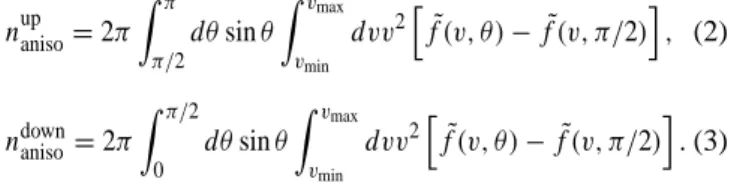
nup_aniso=2π Z π π/2 dθsin θ Z vmax vmin dvv2hf (v, θ ) − ˜˜ f (v, π/2)i, (2) ndown_aniso=2π Z π/2 0 dθsin θ Z vmax vmin dvv2hf (v, θ ) − ˜˜ f (v, π/2)i.(3)

These formulas are valid as written in the Northern Hemi-sphere. In the Southern Hemisphere the θ integration lim-its are replaced by 0..π/2 for nup_aniso and π/2..π for ndown_aniso. The v integral is restricted in a range of velocities vmin ..

vmaxcorresponding to an energy range Emin.. Emaxwhere

Emin,max = (1/2)mev2min,max. The total anisotropic charge density is defined by

naniso=nup_aniso+ndownaniso (4)

and the up-down difference anisotropy by

ndiff_aniso=nup_aniso−ndown_aniso. (5)

Finally, the relative anisotropy is defined by

Arel= naniso n⊥ , (6) where n⊥=2π Z π π/2 dθsin θ Z vmax vmin dvv2f (v, π/˜ 2) =2π Z vmax vmin dvv2f (v, π/˜ 2) (7)

is the “perpendicular density”.

All the naniso quantities have the dimensionality of den-sity, i.e. can be expressed in units of cm−3. Explained in words, the perpendicular distribution function is copied over all pitch angles, subtracted from the distribution function, and the result of the subtraction is integrated over the wanted velocity (energy) range to obtain the partial density corre-sponding to the anisotropic part of the distribution. The quantity ndiff_anisotells how much imbalance in the up/down di-rection there is in the anisotropy: for example, if the aniso-tropy consists of only upgoing electrons, ndiff_aniso=naniso. The

relative anisotropy Arelis a dimensionless number indicating the significance of the anisotropy. It is positive for Tk> T⊥

type anisotropies, equal to zero for isotropic distributions and negative for Tk< T⊥type anisotropies.

The anisotropies, as defined here, can have both positive and negative values. Negative anisotropies (T⊥ > Tk type

anisotropies) turn out to be rare, at least in the middle energy range, and are not discussed in this paper.

3 Specific events

To obtain a more concrete picture of the electron anisotro-pies in the auroral zone, we now study three specific events, collected at radial distances between 3.5 and 5.5 RE, where

the first one represents eveningside, the second one midnight and the third one morningside. Some kind of middle-energy anisotropies can be discerned in almost all auroral crossings. The examples selected here exhibit anisotropies that are a bit stronger and clearer than on the average, but that are not the strongest possible. The examples are from Northern Hemi-sphere, so a zero pitch angle means downward.

3.1 Eveningside event – 8 May 1998

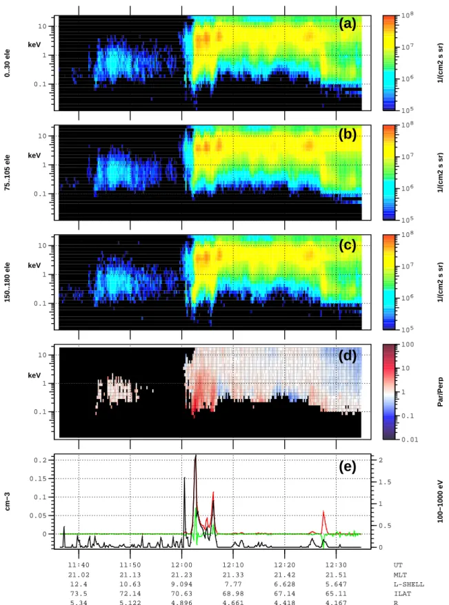
Figure 1 shows the event that occurred on 8 May 1998, 11:35–12:35 UT. Panels (a–c) show the standard HYDRA differential energy flux panels in the downward (pitch an-gle range 0 − 30◦_{), perpendicular (75 − 105}o_{) and upward} direction (150 − 180◦_{) electrons, respectively. From these}

panels it is difficult to detect anisotropies, but they become very clear in panel (d) which is the relative energy-dependent anisotropy, (Eq. 1). The Tk > T⊥type anisotropies that we

are interested in and which are also the most common ap-pear as red. In all HYDRA colour panels, differential energy fluxes which are smaller than 105eV cm−2s−1sr−1eV−1 are shown as black. In panel (d), if either the parallel or the perpendicular differential energy flux is smaller than the limit 105eV cm−2s−1sr−1eV−1, the corresponding relative energy-dependent anisotropy is also shown as black. Ad-ditionally, points having larger than 30% statistical error (points that have less than 10 counts) are shown as black. Thus, values differing from black are guaranteed to repre-sent values that are measured reliably. Panel (e) shows three curves: the anisotropy naniso(red), the up minus down differ-ence anisotropy ndiff_aniso(green) and the relative anisotropy Arel (black). The scale of the red and green curves is on the left (both are in density units) and the scale of the dimensionless black curve is on the right.

In Fig. 1, Polar arrives from the polar cap and en-ters the auroral zone at 12:00 UT in the pre-midnight sec-tor. Rather strong middle-energy anisotropies are detected 12:02–12:07 UT. The anisotropies also extend above 1 keV to some extent (panel d). The middle-energy anisotropy (panel e) reaches 0.2 cm−3 and the relative anisotropy Arel (Eq. 6) has a maximum value of 2. The anisotropies are al-most up/down symmetrical because the difference anisotropy

0.1 1 10 0..30 ele 1/(cm2 s sr) 105 106 107 108 0.1 1 10 75..105 ele _{1/(cm2 s sr)} 105 106 107 108 0.1 1 10 150..180 ele 1/(cm2 s sr) 105 106 107 108 0.1 1 10 Par/Perp 0.01 0.1 1 10 100 11:40 11:50 12:00 12:10 12:20 12:30 UT 0 0.05 0.1 0.15 0.2 0 0.5 1 1.5 2 cm−3 100−1000 eV 21.02 21.13 21.23 21.33 21.42 21.51 MLT 12.4 10.63 9.094 7.77 6.628 5.647 L−SHELL 73.5 72.14 70.63 68.98 67.14 65.11 ILAT 5.34 5.122 4.896 4.661 4.418 4.167 R

(a)

(b)

(c)

(d)

(e)

Fig. 1. HYDRA electron data for 8 May 1998, 11:40–12:35 UT. Panels from top to bottom: differential electron energy flux for (a) downgoing

electrons, (b) perpendicular electrons, (c) upgoing electrons; (d) ratio of parallel to perpendicular differential energy flux (energy-dependent relative anisotropy r(E), Eq. (1)); and (e) three middle-energy anisotropy curves: naniso(red) and ndiff_aniso(green) with scale on the left, and

P. Janhunen et al.: Electron anisotropies in auroral region 241 −5.9×107 _0.0×100 _5.9×107 −5.9×107 0.0×100 5.9×107 ELE 19980508, 12:02:12 .. 12:02:24 vPerp (m/s) vPar (m/s) 1/(cm2 s sr keV2)

Relative original energy 0

1e+03 4e+03 7e+03 1e+04 4e+04 7e+04 1e+05 4e+05 7e+05 1e+06 4e+06 7e+06 1e+07 4e+07 7e+07 1e+08 4e+08 7e+08 1e+09 (a) −5.9×107 _0.0×100 _5.9×107 −5.9×107 0.0×100 5.9×107

ELE 19980508, 12:02:24 .. 12:02:36

Relative original energy 0

1e+03 4e+03 7e+03 1e+04 4e+04 7e+04 1e+05 4e+05 7e+05 1e+06 4e+06 7e+06 1e+07 4e+07 7e+07 1e+08 4e+08 7e+08 1e+09

(b)

Relative original energy 0

1e+03 4e+03 7e+03 1e+04 4e+04 7e+04 1e+05 4e+05 7e+05 1e+06 4e+06 7e+06 1e+07 4e+07 7e+07 1e+08 4e+08 7e+08 1e+09 (c) −5.9×107 _0.0×100 _5.9×107 −5.9×107 0.0×100 5.9×107 ELE 19980508, 12:02:48 .. 12:03:0 vPerp (m/s) vPar (m/s) 1/(cm2 s sr keV2)

Relative original energy 0.0153592 (0.0121−4.959 keV, 24 pts)

1e+03 4e+03 7e+03 1e+04 4e+04 7e+04 1e+05 4e+05 7e+05 1e+06 4e+06 7e+06 1e+07 4e+07 7e+07 1e+08 4e+08 7e+08 1e+09 (d)

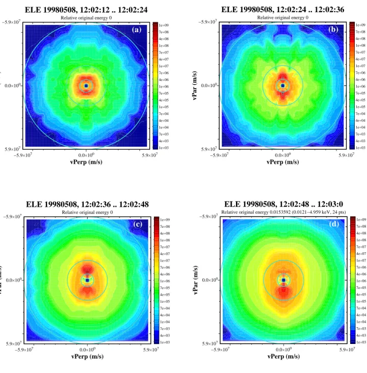
Fig. 2. Electron distribution function (cm−2 s−1 sr−1keV−2) for four successive 12-s intervals on 8 May 1998 event, starting at (a) 12:02:18 UT, (b) 12:02:30, (c) 12:02:42 UT, (d) 12:02:54. Velocities corresponding to 10 eV, 100 eV, 1 keV and 10 keV energies are shown by blue circles; notice that the innermost circle is very small. Magnetic field is oriented downward, parallel to the positive vertical axis, and positive parallel velocity is along the magnetic field, i.e. downward, and the loss cone, if any, appears on the top of each panel.

(green curve in panel e) is smaller than the anisotropy itself, except for a brief moment near 12:27 UT. This example was chosen mainly to demonstrate that occasionally the middle-energy anisotropies can extend to higher than 1 keV energies. Figure 2 shows the electron distribution function at four successive intervals, separated by 12 s, around the strongest anisotropy peak at 12:02–12:03 UT. The four circles where the innermost one is barely visible correspond to 10, 100, 1000 and 10 000 eV energies. The first interval (panel a) dis-plays almost no anisotropy, whereas the second one (panel b)

exhibits a clear middle-energy anisotropy. This anisotropy is slightly atypical in that there are relatively few electrons be-low 100 eV energy. The 3rd interval (panel c) also displays a clear anisotropy, and in the 4th interval (panel d) there still exists anisotropy, with a modest predominantly downward character. Now the anisotropy also extends to higher energies above 1 keV. In all panels an almost isotropic high-energy Maxwellian electron distribution is seen which is likely to be of magnetospheric origin. This is a feature which is nearly invariably associated with the middle-energy anisotropies.

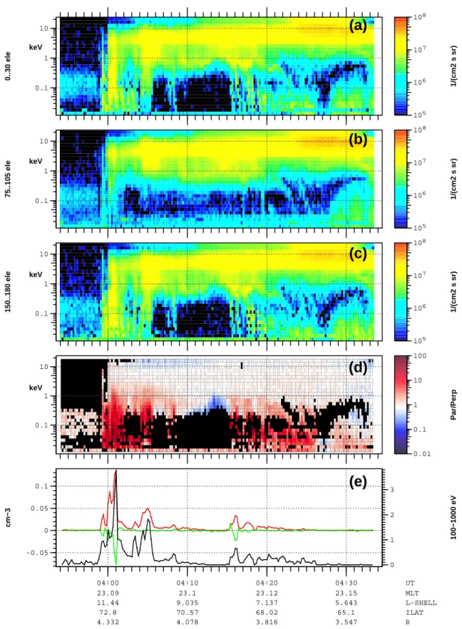
0.1 1 10 0..30 ele 1/(cm2 s sr) 105 106 107 108 0.1 1 10 75..105 ele _{1/(cm2 s sr)} 105 106 107 108 0.1 1 10 150..180 ele 1/(cm2 s sr) 105 106 107 108 0.1 1 10 Par/Perp 0.01 0.1 1 10 100 04:00 04:10 04:20 04:30 UT −0.05 0 0.05 0.1 0 1 2 3 cm−3 100−1000 eV 23.09 23.1 23.12 23.15 MLT 11.44 9.035 7.137 5.643 L−SHELL 72.8 70.57 68.02 65.1 ILAT 4.332 4.078 3.816 3.547 R

(a)

(b)

(c)

(d)

(e)

P. Janhunen et al.: Electron anisotropies in auroral region 243 −5.9×107 _0.0×100 _5.9×107 −5.9×107 0.0×100 5.9×107 ELE 19980422, 04:00:30 .. 04:00:42 vPerp (m/s) vPar (m/s) 1/(cm2 s sr keV2)

Relative original energy 0

1e+03 4e+03 7e+03 1e+04 4e+04 7e+04 1e+05 4e+05 7e+05 1e+06 4e+06 7e+06 1e+07 4e+07 7e+07 1e+08 4e+08 7e+08 1e+09 (a) −5.9×107 _0.0×100 _5.9×107 −5.9×107 0.0×100 5.9×107

ELE 19980422, 04:00:42 .. 04:00:54

Relative original energy 0

1e+03 4e+03 7e+03 1e+04 4e+04 7e+04 1e+05 4e+05 7e+05 1e+06 4e+06 7e+06 1e+07 4e+07 7e+07 1e+08 4e+08 7e+08 1e+09

(b)

ELE 19980422, 04:00:54 .. 04:01:6

Relative original energy 0

1e+03 4e+03 7e+03 1e+04 4e+04 7e+04 1e+05 4e+05 7e+05 1e+06 4e+06 7e+06 1e+07 4e+07 7e+07 1e+08 4e+08 7e+08 1e+09

(c)

Relative original energy 0

1e+03 4e+03 7e+03 1e+04 4e+04 7e+04 1e+05 4e+05 7e+05 1e+06 4e+06 7e+06 1e+07 4e+07 7e+07 1e+08 4e+08 7e+08 1e+09 (d)

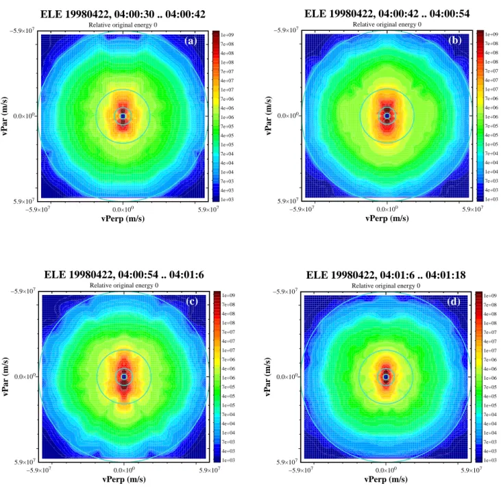
Fig. 4. Electron distribution functions (cm−2s−1sr1keV−2) for four successive 12-s intervals on 22 April 1998: (a) 04:00:36 UT, (b) 04:00:48, (c) 04:01:00, (d) 04:01:12. Same format as in Fig. 2.

The high-energy isotropic electrons have not experienced any parallel acceleration.

3.2 Midnight event – 22 April 1998

Figure 3 shows the event that occurred on 22 April 1998, 03:55–04:35 UT, near the local midnight. The format of the figure is similar to Fig. 1. Again, Polar moves from the polar cap into the auroral zone at 03:58 UT. Strong low and middle-energy anisotropies can be detected over the whole auroral interval. Highest anisotropies occur 03:59–04:01 UT (red line in panel e), when the relative anisotropy Arel(black line

in panel e) reaches almost 4. The strongest peak at 04:01 UT is predominantly downward (negative green curve in panel e), but otherwise the anisotropies are more or less up/down symmetrical.

Figure 4 presents four distribution functions, taken at four successive intervals separated by 12 s around the strongest anisotropy peak 04:01 UT. They show that in this case the anisotropies did not vary as rapidly as in the 8 May 1998 example. All four intervals show roughly similar and rather typical (strong) middle-energy anisotropies.

In this event there are also low-energy up- and downgo-ing electron beams visible in Fig. 3, for example, around

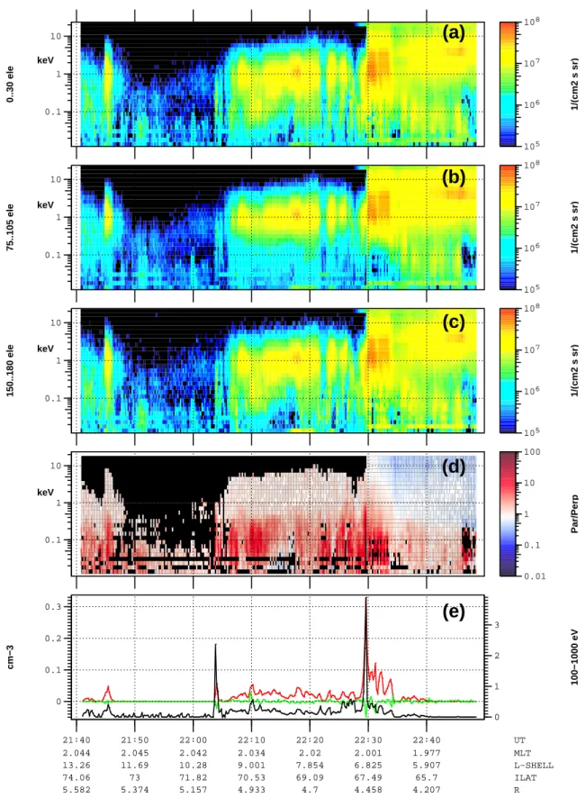
0.1 1 10 0..30 ele 1/(cm2 s sr) 105 106 107 108 0.1 1 10 75..105 ele _{1/(cm2 s sr)} 105 106 107 108 0.1 1 10 150..180 ele 1/(cm2 s sr) 105 106 107 108 0.1 1 10 Par/Perp 0.01 0.1 1 10 100 21:40 21:50 22:00 22:10 22:20 22:30 22:40 UT 0 0.1 0.2 0.3 0 1 2 3 cm−3 100−1000 eV 2.044 2.045 2.042 2.034 2.02 2.001 1.977 MLT 13.26 11.69 10.28 9.001 7.854 6.825 5.907 L−SHELL 74.06 73 71.82 70.53 69.09 67.49 65.7 ILAT 5.582 5.374 5.157 4.933 4.7 4.458 4.207 R

(a)

(b)

(c)

(d)

(e)

P. Janhunen et al.: Electron anisotropies in auroral region 245 −5.9×107 _0.0×100 _5.9×107 −5.9×107 0.0×100 5.9×107 ELE 19980310, 22:29:18 .. 22:29:30 vPerp (m/s) vPar (m/s) 1/(cm2 s sr keV2)

Relative original energy 0

1e+03 4e+03 7e+03 1e+04 4e+04 7e+04 1e+05 4e+05 7e+05 1e+06 4e+06 7e+06 1e+07 4e+07 7e+07 1e+08 4e+08 7e+08 1e+09 (a) −5.9×107 _0.0×100 _5.9×107 −5.9×107 0.0×100 5.9×107

ELE 19980310, 22:29:30 .. 22:29:42

Relative original energy 0

1e+03 4e+03 7e+03 1e+04 4e+04 7e+04 1e+05 4e+05 7e+05 1e+06 4e+06 7e+06 1e+07 4e+07 7e+07 1e+08 4e+08 7e+08 1e+09

(b)

Relative original energy 0

1e+03 4e+03 7e+03 1e+04 4e+04 7e+04 1e+05 4e+05 7e+05 1e+06 4e+06 7e+06 1e+07 4e+07 7e+07 1e+08 4e+08 7e+08 1e+09 (c) −5.9×107 _0.0×100 _5.9×107 −5.9×107 0.0×100 5.9×107

ELE 19980310, 22:29:54 .. 22:30:6

Relative original energy 0

1e+03 4e+03 7e+03 1e+04 4e+04 7e+04 1e+05 4e+05 7e+05 1e+06 4e+06 7e+06 1e+07 4e+07 7e+07 1e+08 4e+08 7e+08 1e+09

(d)

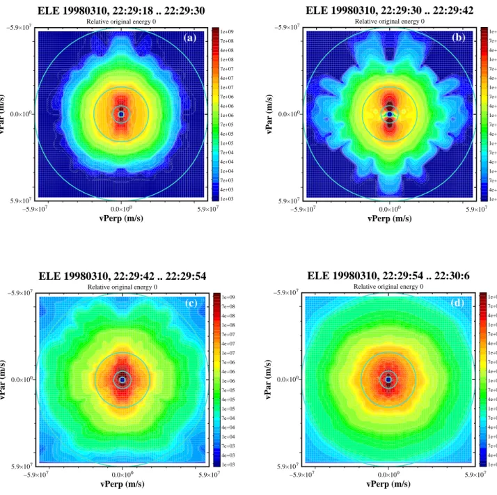
Fig. 6. Electron distribution functions (cm−2s−1sr1keV−2) for four successive 12-s intervals on 10 March 1998: (a) 22:29:18 UT, (b) 22:29:36, (c) 22:29:48, (d) 22:30:00. Same format as in Fig. 2.

04:18 UT. Since this activity is below 100 eV, it does not con-tribute to panel (e).

3.3 Morningside event – 10 March 1998

Figure 5 shows an event that occurred on 10 March 1998, 21:40–22:45 UT, in the post-midnight sector. There is aniso-tropy all the way from 22:05 to 22:35 UT. The strongest peak appears close to 22:30 UT. The anisotropies during this event are at somewhat lower energies than in the other two exam-ples, now extending all the time, also well below 100 eV, and

there are hardly any anisotropies above 1 keV, even though strong electron fluxes exist around 1 keV (see the top three panels).

The distribution functions taken around 22:30 UT (Fig. 6) show how the anisotropy grows and reaches its peak and then suddenly becomes reduced. At the same time the temper-ature of the high-energy electron population increases (or a new population appears). When the anisotropy reaches its peak (panel b) the whole distribution is irregular, which sug-gests that rapid temporal variations are going on during this 12-s integration.

66 67 68 69 70 71 72 73 ILAT nAnisoHigh (cm−3) 0 0.0005 0.001 0.0015 0.002 0.0025 0.003 66 67 68 69 70 71 72 73 ILAT nAnisoMid (cm−3) 0 0.005 0.01 0.015 0.02 0.025 66 67 68 69 70 71 72 73 ILAT nAnisoLow (cm−3) 0 0.05 0.1 0 5 10 15 20 MLT 66 67 68 69 70 71 72 73 ILAT Orb. coverage (h) 0 5 10 15 20 25 30

Fig. 7. 90th percentiles of electron anisotropies in different

en-ergy ranges as a function of MLT and ILAT and integrated over radial distances 2.5 − −6R_E, for high-energy (1–10 keV; top panel), middle-energy (100–1000 eV; second panel), low-energy (10–100 eV; third panel). The bottom panel shows the orbital cov-erage in hours. The 90th percentile is defined as the value which is such that 90% of the measured values are smaller and 10% are larger.

In all three events presented, strong anisotropy peaks ac-company the polar cap boundary, which is sharply defined. Among auroral crossings of Polar, this kind of behaviour is relatively common, although by no means a rule. Also, in the events shown, some of the anisotropy peaks occur together with sudden changes in the high energy electron distribution. This behaviour is not very typical, but occurs only in some events.

4 Statistical results

4.1 MLT and ILAT

Figure 7 shows the distribution of the 90th percentile of the electron anisotropies for three energy ranges, as a function of MLT and ILAT. The bottom panel shows the number of hours measured by the instrument in each bin. The radial distance range included in the plot is 2.5 − 6RE. The 90th percentile

is defined as the value which is such that 90% of the mea-sured values are smaller and 10% are larger. The motivation for selecting the 90th percentile is that 10% is the typical

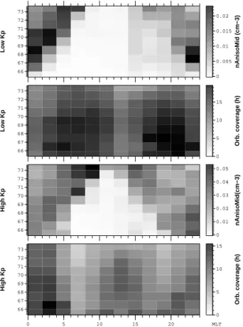
oc-66 67 68 69 70 71 72 73 Low Kp nAnisoMid (cm−3) 0 0.005 0.01 0.015 0.02 66 67 68 69 70 71 72 73 Low Kp Orb. coverage (h) 0 5 10 15 66 67 68 69 70 71 72 73 High Kp nAnisoMid(cm−3) 0 0.01 0.02 0.03 0.04 0.05 0 5 10 15 20 MLT 66 67 68 69 70 71 72 73 High Kp Orb. coverage (h) 0 5 10 15

Fig. 8. Middle-energy (100–1000 eV) anisotropy dependence on

Kp index. First panel: 90th percentile of middle-energy (100–

1000 eV) anisotropies for low Kp (Kp ≤ 2), second panel:

or-bital coverage for low Kp, third panel: 90th percentile for high Kp

(Kp>2), fourth panel: orbital coverage for high Kp. The vertical

axis in each panel is the invariant latitude (ILAT).

currence frequency of auroral arc-related phenomena within the auroral zone. If one uses the 75th percentile (i.e. the upper quartile) instead of the 90th percentile, for example, the values in all panels become smaller but the patterns re-main qualitatively very similar. The high-energy range (top panel) has the lowest values for the anisotropy, and these an-isotropies occur mainly near the midnight auroral zone. The middle-energy anisotropies (second panel from the top) fol-low the auroral oval pattern, with a clear MLT dependence, with anisotropies being more common around midnight than elsewhere. The third panel from top shows the low-energy anisotropies, which are seen to be mainly a dayside phe-nomenon, being more common in the pre-noon sector than in the post-noon sector. Although the dayside is not the primary emphasis of this paper we remark that the preference of the low-energy anisotropies to appear before noon might be due to E × B-drifting cold plasma flowing away from the Earth in the post-noon sector which follows from the combined effect of magnetospheric convection and corotation (Kivelson and Russell (1995), Fig. 10.25 on p. 316).

The high-energy anisotropies could possibly give rise to potential structures of large magnitude, if the density

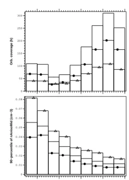
imbal-P. Janhunen et al.: Electron anisotropies in auroral region 247 [t] 0 50 100 150 200 250 300 Orb. coverage (h) 2 3 4 5 6 R/R_E 0 0.01 0.02 0.03 0.04 0.05 0.06 0.07 0.08 90−percentile of nAnisoMid (cm−3)

Fig. 9. Bottom panel: Radial dependence of the 90th percentile of

middle-energy (100–1000 eV) anisotropies for small Kp(solid line

with filled circles, Kp≤2) and large Kp(solid line with triangles, Kp>2) measured at 65:74 ILAT and 18:06 MLT. Solid line

with-out symbols shows results for low and high Kpcombined together.

Top panel: Orbital coverage in hours in each radial bin.

ance produced by them exceeds the colder component densi-ties at some altitude (at low enough altitude one can always find cold plasma, so the question is not whether cold plasma exists but at what altitude it exists). However, the anisotropic densities are so small that this is not likely to happen. Thus, the high energy anisotropies are probably not very significant as far as auroral potential structures are concerned.

The low-energy range (10–100 eV) probably cannot be trusted completely, since it is affected, for example, by the spacecraft potential. It is possoble that the anisotropies that we call “middle-energy” actually rather often extend below 100 eV, although the instrument cannot always reliably detect them.

If one produces a plot similar to Fig. 7 separately for up-going and downup-going anisotropies nup_anisoand ndown_aniso, the plots are nearly identical, i.e. there is no clear difference in the sta-tistical properties of upgoing and downgoing anisotropies. 4.2 Kp

Figure 8 shows how the middle-energy (100–1000 eV) aniso-tropy 90th percentile depends on the Kp index. We see that

when Kpincreases, the middle-energy anisotropies move

to-wards lower latitudes. This is a further confirmation that the middle-energy anisotropies are associated with auroral pro-cesses, since the auroral oval also resides at lower latitudes during high Kp (Feldstein and Starkov, 1967). The

aniso-tropy magnitude generally increases with an increasing Kp

index.

4.3 Other effects

Without showing plots, we mention a few results for the an-isotropies. First, the middle-energy anisotropies are almost symmetric in the up/down direction, which means that most of the electrons do not precipitate into the atmosphere or originate from it. Second, there is no clear solar illumination dependence, saying that it is not important to the anisotropy results whether or not the ionospheric footpoint is sunlit. 4.4 Altitude dependence

The bottom panel of Fig. 9 shows the 90th percentile of the middle-energy anisotropies against the geocentric radial dis-tance R for small (≤ 2) and large (> 2) Kp values. The top

panel presents the number of hours the satellite spent in each 0.5RE radial distance bin. We notice that for increasing Kp

the anisotropy magnitude increases. Furthermore, the aniso-tropy magnitude increases with decreasing altitude, which is natural because the stronger the anisotropy (the larger the ra-tio Tk/T⊥), the more the density follows the flux tube scaling

(Eq. (7) and Fig. 1 of Janhunen and Olsson, 2002a). It could also partly be caused by failing to detect very field-aligned anisotropies at high altitudes, because one of the detectors is not always looking exactly at field-aligned direction. No-tice also that the high-altitude anisotropies should be more field-aligned than the low-altitude ones because of the mirror force.

5 Summary and discussion

In this paper we have investigated middle-energy electron anisotropies in the auroral zone, using observations of elec-tron distribution functions by the HYDRA instrument from the Polar satellite and using a novel definition of anisotropy which is capable of quantifying anisotropies occurring in a limited energy range. The major findings are as follows.:

1. Most often the Tk> T⊥type anisotropies are limited to

a certain energy range, typically ∼ 100–1000 eV. 2. Almost always there is simultaneously an isotropic

elec-tron distribution at higher energies.

3. Often the anisotropies are up/down symmetric, although cases with net upward or downward electron flow also occur.

4. The MLT-ILAT distribution of middle-energy anisotro-pies (100–1000 eV) obeys that of the average auroral oval (Fig. 7). The distributions of the low and high-energy anisotropies are more irregular. This suggests that it is specifically the middle-energy anisotropies that have something to do with auroral acceleration pro-cesses.

5. When the Kpindex increases, the middle-energy

aniso-tropies appear at lower ILAT in all MLT sectors, as is expected for an auroral oval related process. Their 90th percentile also increases with increasing Kp.

6. The altitude dependence of the anisotropies is smooth as one would expect, because the electrons have high mo-bility along the magnetic field and thus the anisotropies spread rapidly to different altitudes.

7. Within the auroral zone and at about 4 RE radial

dis-tance, the 90th percentile of the middle-energy (100– 1000 eV) anisotropic density is ∼ 0.02 − 0.03 cm−3_. The anisotropic density decreases with increasing radial distance R, so that it is roughly proportional to R−1.8, which can be deduced from Fig. 9.

In order to assess the role of the middle-energy anisotro-pies further using observational studies, one should find their statistical correlation with other phenomena occurring on au-roral field lines, such as broad-band wave activity. If the waves are producing the anisotropies, then there should exist a correlation between them, as is recently found in an event study by Janhunen et al. (2001).

A possible mechanism for producing middle-energy elec-tron anisotropies is to have waves whose parallel phase ve-locity is in Landau resonance with the thermal speed of elec-trons. Recent particle simulations have shown that ion Bern-stein waves driven to be unstable by a hot ion shell distribu-tion can energise ∼ 100 eV electrons at a rate of 80 eV/s (Jan-hunen et al., 2003a). Since the travel time of a 100 eV elec-tron (parallel energy) through the altitude range of, say, 4 RE

is 4 s, such electrons may gain several hundred eV of extra parallel energy during one trip through the region. Because of the mirror force and convergent flux tube geometry, par-allel electron energisation should also produce macroscopic charge separation effects. It has been demonstrated using a special type of electrostatic hybrid simulations that parallel electron energisation may lead to self-consistent auroral po-tential structure formation (Janhunen and Olsson, 2002a).

If one tries to build a synthesis of the new results men-tioned in this paragraph, the following picture tends to emerge: (1) Ion Bernstein or lower hybrid waves are driven unstable by some free energy source, possibly a hot ion shell distribution (Janhunen et al., 2003a). One way to produce ion shell distributions is by time of flight effects of ions in-jected from the reconnection X line. (2) Middle-energy elec-trons (the present paper) are energised by the waves in the parallel direction with a Landau resonance mechanism (Jan-hunen et al., 2001, 2003a). (3) The parallel energisation of electrons leads to charge separation effects and auroral po-tential structure formation taking place below ∼ 4 RE

ra-dial distance (Janhunen et al., 1999; Janhunen and Olsson, 2002a). (4) The presence of the potential structure gives the characteristic inverted-V shape to low-altitude electron dis-tributions (Janhunen and Olsson, 2000), generates upgoing ion beams (Janhunen et al., 2003b) and a density cavity (Jan-hunen et al., 2002b). Alfv´enic wave acceleration probably

modifies this picture in dynamic events such as substorm on-sets. The middle-energy electron anisotropies are thus one important link in a relatively complicated chain of energy flow from the reconnection X-line to inverted-V electron pre-cipitation.

Acknowledgements. We are grateful to Craig Kletzing for

provid-ing the HYDRA data and for givprovid-ing many useful comments. The work of PJ was supported by the Academy of Finland and that of AO and AV by the Swedish Research Council.

The Editor in Chief thanks V. Sergeev and another referee for their help in evaluation this paper.

References

Alfv´en, H. and F¨althammar, C. G.: Cosmical Electrodynamics, Clarendon, Oxford, 1963.

Collin, H. L., Sharp, R. D., and Shelley, E. G.: The occurrence and characteristics of electron beams over the polar regions, J. Geophys. Res., 87, 7504–7511, 1982.

Feldstein, Y. I. and Starkov, G. V.: Dynamics of auroral belt and polar geomagnetic disturbances, Planet. Space Sci., 15, 209–229, 1967.

Hada, T., Nishida, A., Terasawa, T., and Hones, E .W., Jr.: Bi-directional electron pitch angle anisotropy in the plasma sheet, J. Geophys. Res., 86, 11 211–11 224, 1981.

Janhunen, P., Olsson, A., Mozer, F. S., and Laakso, H.: How does the U-shaped potential close above the acceleration region? A study using Polar data, Ann. Geophysicae, 17, 1276–1283, 1999. Janhunen, P., Olsson, A. W., Peterson, K., Laakso, H., Pickett, J. S., Pulkkinen, T. I., and Russell, C. T.: A study of inverted-V auro-ral acceleration mechanisms using Polar/Fast Auroauro-ral Snapshot conjunctions, J. Geophys. Res., 106, 18 995–19 011, 2001. Janhunen, P. and Olsson, A.: New model for auroral acceleration:

O-shaped potential structure cooperating with waves, Ann. Geo-physicae, 18, 596–607, 2000.

Janhunen, P. and Olsson, A.: A hybrid simulation model for a stable auroral arc, Ann. Geophysicae, 20, 1603–1616, 2002a.

Janhunen, P., Olsson, A., and Laakso, H.: Altitude dependence of plasma density in the auroral zone, Ann. Geophysicae, 20, 1743– 1750, 2002b.

Janhunen, P., Olsson, A., Vaivads, A., and Peterson, W. K.: Gener-ation of Bernstein waves by ion shell distributions in the auroral region, Ann. Geophysicae, in press, 2003a.

Janhunen, P., Olsson, A., and Peterson, W. K.: The occurrence fre-quency of upward ion beams in the auroral zone as a function of altitude using Polar/TIMAS and DE-1/EICS data, Ann. Geo-physicae, in press, 2003b.

Kivelson, M. and Russell, C. T.: Introduction to space physics, Cambridge University Press, 1995.

Kletzing, C. A. and Scudder, J. D.: Auroral-plasma sheet electron anisotropy, Geophys. Res. Lett., 26, 971–974, 1999.

Klumpar, D. M., Quinn, J. M., and Shelley, E. G.: Counter-streaming electrons at the geomagnetic equator near 9 RE, J.

Geophys. Res., 93, 1295–1298, 1988.

Lin, C. S., Mauk, B., Parks,G. K., DeForest, S., and McIlwain, C. E.: Temperature characteristics of electron beams and ambient particles, J. Geophys. Res., 84, 2651–2654, 1979.

Marklund, G. T. and Karlsson, T.: Characteristics of the auroral par-ticle acceleration in the upward and downward current regions, Phys. Chem. Earth, 26, 81–96, 2001.

P. Janhunen et al.: Electron anisotropies in auroral region 249

Richardson, J. D., Fennell, J. F. and Croley, Jr., D. R. : Observations of field-aligned ion and electron beams from SCATHA (P78-2), J. Geophys. Res., 86, 10 105–10 110, 1981.

Scudder, J. D., Hunsacker, F., Miller, G., Lobell, J., Zawistowski, T., Ogilvie, K., Keller, J., Chornay, D., Herrero, F., Fitzenreiter, R., and 12 coauthors: Hydra - A 3-dimensional electron and ion hot plasma instrument for the Polar spacecraft of the GGS mission, Space Sci. Rev., 71, 459–495, 1995.

Sergeev, V. A., Baumjohann, W., and Shiokawa, K.: Geophys. Res. Lett., 28, 3813–3816, 2001.

Sharp, R. D., Shelley, E. G., Johnson, R. G., and Ghielmetti, A. G.: Counterstreaming electron beams at altitudes of ∼ 1REover the

auroral zone, J. Geophys. Res., 85, 92–100, 1980.

Whipple, E.C., Jr.: The signature of parallel electric fields in a col-lisionless plasma, J. Geophys. Res., 82, 1525–1531, 1977.