Effect of chemical mechanical planarization processing conditions on polyurethane pad properties

Effect of Chemical Mechanical Planarization Processing Conditions

on Polyurethane Pad Properties

by

Grace Siu-Yee Ng

S.B., Materials Science and Engineering Massachusetts Institute of Technology, 2002

Submitted to the Department of Materials Science and Engineering In Partial Fulfillment of the Requirements for the Degree of

Master of Science in Materials Science and Engineering at the

Massachusetts Institute of Technology June 2003

© Grace S. Ng. All rights reserved.

MASSACHUSETS INSTITUTE OF TECHNOLOGY

JAN

0 7

2003O

LIBRARIES

The author hereby grants to MIT permission to reproduce and to distribute publicly paper and electronic copies of this thesis document in whole or in part.

Signature of Author:

Department of aterials Science Engineering

V _{May 9, 2003}

Certified by:

David K. Roylance Associate Professor of aterials Engineering

I Thelis Supervisor

Accepted by:

1t-rry L. Tuller Professor of Ceramics and Electronic Engineering Chairman, Committee for Graduate Students

Effect of Chemical Mechanical Planarization Processing Conditions on Polyurethane Pad Properties

by

Grace Siu-Yee Ng

Submitted to the Department of Materials Science and Engineering On May 9, 2003 in partial fulfillment of the

requirements for the Degree of Master of Science in Materials Science and Engineering

ABSTRACT

Chemical Mechanical Planarization (CMP) is a vital process used in the semiconductor industry to isolate and connect individual transistors on a chip. However, many of the fundamental mechanisms of the process are yet to be fully understood and defined. The difficulty in analyzing the CMP process lies in the fact that many factors, such as properties of consumables, polishing speed, polishing pressure, etc, can affect the outcome of the CMP process. This paper focuses on the thermal and mechanical

properties of one of the consumables - the CMP soft pad. During the CMP process, the pad is subjected to high temperatures and chemicals from the slurry. Thus, the properties of the pad can be irreversibly changed, affecting the planarity of the resultant wafer. In this study, the CMP processing conditions were simulated in the laboratory by annealing the pad at high temperatures and soaking the pad in slurry and DIW for up to two months. The properties of the CMP pad were then measured using four thermoanalytical tools

-dynamic mechanical analyzer (DMA), gravimetric analyzer (TGA), thermo-mechanical analyzer (TMA), and modulated differential scanning calorimeter (MDSC). Results suggested that both annealing at temperatures above 1400_{C and soaking in slurry} for up to two weeks significantly increase the storage modulus of the sample and promote pad shrinkage in the transverse dimension. Thus, it is not recommended that the soft pad be used at operating temperatures above 1400_{C and for polishing times of more than two}

weeks (336 hrs).

Thesis Supervisor: David K. Roylance

TABLE OF CONTENTS

LIST OF FIGURES...5

ACKNOWLEDGEM ENTS...6

CHAPTER 1 : INTRODUCTION...7

1.1 Driving Force Behind Chemical Mechanical Planarization (CMP) Improvement... 7

1.2 Growing CMP Market ... ... 8

CHAPTER 2: BACKGROUND...9

2.1 C M P Process...9

2.1.1 Factors Effecting Materials Removal...10

2.1.2 Motivations for Study...11

2.2 Polym er Physics... ... 13 2.2.1 Formation of Polyurethane...13 2.2.2 Types of Polyurethane...14 2.2.2.1 Foam s...14 2.2.2.2 Solid Polyurethanes ... ... 15 2.2.3 Cross-linking in Polyurethane...15

2.2.3.1 Dependence of Glass Transition Temperature (Tg) Upon Cross-linking Density ... 16

CHAPTER 3: EXPERIMENTAL...19

3.1 M aterials... 19

3.2 Procedure...19

3.2.1 Pad Uniformity Test...20

3.2.2 A nneal Test... ... 21

3.2.3 Soak Test...21

3.3 Characterization... 21

3.3.1 Diffusion Analysis ... 22

3.3.2 Thermo-gravimetric Analysis (TGA)...22

3.3.2.1 General Description...22

3.3.2.2 Experimental Setup...22

3.3.3 Thermo-mechanical Analysis (TMA)...23

3.3.3.1 General Description...24

3.3.3.2 Experimental Setup...24

3.3.4 Dynamical Mechanical Analysis (DMA)...24

3.3.4.1 General Description...24

3.3.4.2 Experimental Setup...26

3.3.5 Modulated Differential Scanning Calorimetry (MDSC)...26

3.2.5.1 General Description...26

3.2.5.2 Experimental Setup...27

CHAPTER 4: RESULTS AND DISCUSSION...28

4.1 Pad Uniformity Test... ... 28

4.2 A nneal Test...30

4.2.1 TGA Results...30

4.2.2 TMA Results...31

4.2.3 DMA Results...33

4.3 Soak Test ... ... 38 4.3.1 Diffusion Analysis ... ... 38 4.3.2 Effect of Slurry... 40 4.3.2.1 TGA Results... ... 40 4.3.2.2 TM A Results... ... 41 4.3.2.3 DMA Results... ... 42 4.3.2.4 MDSC Results... ... 45 4.3.3. Effect of DI W ater... ... 47 4.3.3.1 TGA Results... ... 47 4.3.3.2 TM A Results... ... 47 4.3.3.3 DM A Results... ... 48 4.3.3.4 MDSC Results... ... 50

CHAPTER 5: CONCLUSIONS AND RECOMMENDATIONS...51

5.1 Pad Uniform ity ... ...51

5.2 Effect of Annealing on Pad Properties... ... 51

5.3 Effect of Soaking on Pad Properties... ... 52

CHPATER 6: SOURCES OF ERROR / FUTURE STUDY...53

LIST OF FIGURES

Figure 1 Schematic of CMP process...9

Figure 2 Formation of a polyurethane polymer... ... ... 13

Figure 3 Molecular structure ofpolyurethane... ... ... ... ... ... 15

Figure 4 Variation ofshear modulus and tan 6 with temperature... ... ... ... 17

Figure 5 Variation of Young's modulus with temperature... ... ... ... ... ... 18

Figure 6 Schematic of CMP soft pad... ... ... ...19

Figure 7 Schematic of CMP soft pad divided into three regions... ... ... 20

Figure 8 Schematic of thermobalance... ... ... ... 23

Figure 9 Typical DMA raw data output ... ... ... 28

Figure 10 Plot of average storage modulus vs. location on pad... ... ... 29

Figure 1 I Plot of variation in storage modulus by pad location . ... ... ...30

Figure 12 TGA data for annealedsamples... . . . ... 31

Figure 13 TMA data for annealed samples... .... ... ... ... ... ... ... . ... ... ... ... 32

Figure 14 DMA data for tensile deformation test on annealed samples ... ... ... ... ... ... 33

Figure 15 Plot ofstorage modulus at 300 C vs. annealing temperature... ... ... 34

Figure 16 Plot ofrelative change in storage modulus at 700C vs. annealing temperature...35

Figure 17 Tan 6 curves for annealed samples... ... ... ... ... .. . ... ... ... ... ... ... 35

Figure 18 MDSC data for annealed samples... ... ... ... ... ... ... 36

Figure 19 MDSC data for first heat run of annealed samples ... ... ... 37

Figure 20 Plot of irreversible heat of reaction vs. annealing temperature... ... ... ... ... 38

Figure 21 Plot of weight percent gain vs. square root of soak time... ... ... 39

Figure 22a Schematic of cross section of CMP pad... ... ... 40

Figure 22b SEM image of cross section of CMP pad... ... ... 40

Figure 23 TGA data for samples soaked in slurry... . . ... 41

Figure 24 TMA data for samples soaked in slurry... ... ... ... ... 41

Figure 25 Plot of storage modulus at 300C vs. soak time in slurry ... ... ...43

Figure 26 Plot of storage modulus at 70oC vs. soak time in slurry ... ... .... 43

Figure 27 Tan 3 curves for samples soaked in slurry.. ... ... ... ... ... 44

Figure 28 MDSC data from first heat run of samples soaked in slurry... ... ... ... ... ... 45

Figure 29 Plot of irreversible heat of reaction vs. soak time in slurry... ... ... ... ... ... 46

Figure 30 TGA data for samples soaked in DIW...47

Figure 31 TMA data for samples soaked in DIW... ... . ...48

Figure 32 Plot ofstorage modulus at 300 C vs. soak time in DIW ... ... ... 48

Figure 33 Plot ofstorage modulus at 700_{C vs. soak time in DIW... ... ... ... 49}

Figure 34 Tan 6 curves for samples soaked in DIW... ... ... ... ... ... ... ... 50

ACKNOWLEDGEMENTS

The past five years at M.I.T. have been an incredible journey filled with highs and lows. I would not have been able to survive these years without the help and support of my loving family and friends. I would like to dedicate this paper to my family, friends, and colleagues, who have touched my life in so many ways along this amazing journey. I would like to express my appreciation to my thesis advisor, Professor David K. Roylance, for his understanding, support, and guidance throughout the writing of this thesis. I would also like to express my gratitude to Intel Corporation for giving me the opportunity to perform my research in the Fab Materials Operation (FMO) organization. My appreciation also extends to my Intel supervisor, Alexander Tregub, for his

mentorship during my six month internship at Intel.

More importantly, I would like to thank Mom and Dad for their boundless love and support. Thank you for always believing in me and encouraging me to be the best that I can be, and for putting up with my temper tantrums and impatience when times were rough. To Peter, my big brother, thank you for being a role model for me all these years.

As for my friends, I would like to express my thanks to my fellow course 3ers, Nina, Brad, Amy, and Kenny, whom I shared many long nights of tooling on problem

sets and projects. Special thanks to my roommate, Judy, who has a talent for making me smile and laugh even when I was stressed out. Thanks to Judy C., who was always there to listen and comfort when I was frustrated and wanted to give up. Thanks to Cheng-Han, whose endless supply of Ankara's frozen yogurts kept me energized late into the night. Thanks to Caroline and Anita, whose prayers and encouragements kept me going when times were rough. And thanks to Yee, who always has a smile for me.

Above all, I would like to thank my Heavenly Father for blessing me with so many wonderful friends these past five years. Without His love and grace, I would not be able to make it thus far.

CHAPTER 1 : INTRODUCTION

Planarization is the process of smoothing and planing surfaces. Chemical mechanical planarization (CMP) is the process of smoothing and planing aided by chemical and mechanical forces. Historically, CMP has been used to polish a variety of materials for thousands of years. For example, CMP has been used to produce mirror finished surfaces. Nature runs its own CMP processes to produce beautifully finished stones, created by years of exposure to relatively gentle chemical and mechanical forces. More recently, both optically flat, damage-free glass and semiconductor surfaces have been prepared by the use of CMP processes. Now CMP is being used widely in planarizing the interlayer dielectric (ILD) and metal used to form interconnections between devices and between the devices and the environment.

1.1 Driving Force Behind CMP Improvement

The use of copper as an interconnect material in multilevel integrated circuits is being increasingly considered mainly due to its low resistivity and high resistance to electromigration compared to the widely used aluminum alloys [1 and 2]. As devices become smaller and their architectures become more complicated, conductors on the chips must shrink to occupy less space [3]. Such miniaturization of the conductors causes an increase in the RC delay, defined as the product of the metal resistance (R) and the capacitance (C) of the interlayer dielectric. While the copper is expected to exhibit lower interconnect delay due to its low resistivity, its high resistance to electromigration enhances the device reliability by increasing the mean time to device failure. Therefore,

copper has enormous potential in making integrated circuit for sub-0.5 micron level technology with reduced interconnect delay and maximized circuit performance [2, 4,

and 5]. For potential utilization of copper as an interconnect material, the wafer surface must be made planar on a global scale. The application of reactive ion etching for achieving such global planarity on copper was attempted by previous researchers [6, 7, and 8]. However, the absence of a volatile copper species in the temperature range of reactive ion etching increases process complexity, rendering it uneconomical [9]. Inlaid metal patterns in multilevel chips can be obtained by chemical-mechanical planarization, also known as chemical-mechanical polishing. Hence, the CMP process remains the only viable approach for the global patterning of copper [10].

1.2 Growing CMP Market

In the past decade, CMP has emerged as the fastest-growing operation in the semiconductor manufacturing industry [11]. It is estimated that more than 150 million planarization operations will be conducted in the year 2002, and that number is expected to double in the following three years [12]. This rapid increase will be fueled by the introduction of copper-based interconnects for logic and other devices. The market size for CMP equipment and consumables (slurries, pads, etc.) grew from $250 million in 1996 to over $1 billion in 2000 [13]. In spite of the dramatic market growth and

advancements in processing technology, CMP remains one of the least understood areas in the semiconductor industry [14]. Specifically, the understanding of wafer-pad-slurry interactions that occur during the CMP process remains incomplete. This lack of understanding is a significant barrier to optimizing the wafer planarization process.

CHAPTER 2: BACKGROUND

2.1 CMP Process

Chemical mechanical planarization, as the name suggests, combines both

chemical and mechanical interactions to planarize metal and dielectric surfaces. During this process uses slurry composed of abrasive particles such as silica or alumina, along with a number of chemicals such as oxidizers, surfactants, polymer additives, pH stabilizers, salts, and dispersants [15]. A schematic of the CMP operation is shown in Figure 1.

Slurry / DIW

16afe

Wafer

Figure 1 -A schematic illustration of the CMP process

The polishing slurry is fed onto a polishing pad made of a porous polyurethane based polymer. By moving the pad across the wafer in a circular, elliptical, or linear motion, the wafer surface is polished. The polymeric pad performs several functions,

including uniform slurry transport, distribution and removal of the reacted products, and uniform distribution of applied pressure across the wafer. In a typical CMP process, the chemicals interact with the material to form a chemically modified surface.

Simultaneously, the abrasives in the slurry mechanically interact with the chemically modified surface layers, resulting in material removal [16].

A better understanding of the CMP process can be developed by examining the wafer-pad-slurry interaction at the micro- and nanoscale levels. At the microscale level, the rough pad carrying the particle-based slurry interacts with the surface of the wafer. It is generally believed that the particles, located between the wafer and the pad, remove excess material via a mechanical abrasion process. At the nanoscale level, the kinetics of the formation and removal of the thin surface layer controls CMP output parameters such as removal rate, surface planarity, surface directivity, and slurry selectivity (the polishing rate of the top layer as compared with the underlying layer) [17].

2.1.1 Factors Affecting Materials Removal

There are several factors that affect the material removal procedure, such as chemical and/or mechanical effects of contact pressure, relative velocity, types of pad, and slurry, polishing temperature, and other process conditions [15]. Currently, the most widely used equation for CMP is Preston's Law, which states that the removal rate of a material is directly proportional to the applied pressure and relative velocity of the particles across the wafer [17]. This equation was first suggested nearly 75 years ago for determining material removal when two plates were rubbed against each other.

CMP process. The first constraint in this equation is that the equation was developed for mechanical polishing only, and thus, did not take into account for the chemical

synergistic effects of CMP. Second, the equation fails to provide any insight into the effect of particle size, properties of the slurry, and pad conditions on the polishing process. Although the basics of the process seem simple, the large number of input variables creates a challenge to engineers and scientists in the semiconductor industry.

2.1.2 Motivations for Study

Since the properties of the consumables (slurry and pads) directly affect the CMP process, one approach to optimize the CMP process is to optimize the properties of the consumables (mainly slurry and pads) [18]. This, in turn, depends heavily on reliable characterization of the consumables.

Although all three basic CMP components are equally important, the pad

characteristics are the least understood [16]. The pad plays a major role in controlling the rate and quality of planarization, including instances of feature rounding, dishing,

scratches, and other defects.

During the CMP process, the pad can be subjected to high temperatures due to mechanical friction between the polymer-based pad and a silicon wafer in the solid-solid contact mode [19]. Additionally, exothermic chemical reactions between the slurry and the polished metal can also attribute to pad heating [20]. It has been found empirically that the slurry temperature increases by approximately 20-700_{C during CMP. These}

values reflect the average temperature over the pad/wafer contact area. Due to the

contact with the wafer during the CMP process [21 ]. Thus, in these localized points of contact, temperatures can increase significantly during CMP. These heating effects can be partially alleviated in the hydrodynamic contact mode, due to slurry flow [19].

In addition to temperature increase during the CMP process, CMP pads are also subjected to structural changes due to interactions with the chemical agents in slurry, as well as with water during the rinsing process [22]. Specifically, structural changes of the pads can take place due to plasticizing or cross-linking of the polymer chains, thus

affecting the physical and mechanical properties of the CMP pads. Each wafer is roughly polished for a total of five minutes, and the pad is then rinsed with de-ionized water (DIW) for approximately two minutes. The same pad is reused for as many as 1000 wafers and has an approximate life time of four weeks of continuous use [23]. Within these four weeks, chemical restructuring of the polymer pads is likely to occur.

Since pad heating and/or soaking in slurry/DIW can substantially and irreversibly change the physical and mechanical properties of the CMP pads [24] as well as their chemical structure, it is important to examine the direct impact of the CMP environment on pad properties in order to optimize the CMP pad performance. This, in turn, optimizes the planarity of the finished wafers [18].

This study was conducted to determine the effect of the CMP environment on the thermal and mechanical properties of the CMP pads. Since it is not economically

feasible to analyze the properties of the CMP pad in situ, the pad was subjected to temperature and time conditioning, as well as a soak in tungsten slurry and DIW for

different time intervals in the laboratory to simulate the CMP processing environment. The thermal and mechanical properties of the CMP pad were then analyzed using a set of

four thermoanalytical tools - dynamic mechanical analyzer (DMA), modulated differential scanning calorimeter (MDSC), thermo-mechanical analyzer (TMA), and thermo-gravimetric analyzer (TGA).

2.2 Polymer Chemistry

A polymer is a material composed of molecules which have long sequences of

one or more species of atoms or groups of atoms linked to each other by primary, usually covalent, bonds. These macromolecules are formed by linking together monomer

molecules through chemical reactions, in a process known as polymerization [25].

2.2.1 Formation of Polyurethane

Currently, one of the most commercially useful polymers is polyurethane. Figure 2 depicts a schematic diagram of the formation process of a polyurethane polymer.

S0 OH HO

1I

11

Il

l

I11

CN-- R -NC

+HO-

R-- OH -*

OCN - R - NCO-- R

Polyol Diisocynate Polyurethane

Figure 2 - The formation ofa polyurethane polymer

A urethane linkage is formed by the chemical reaction between an alcohol and an isocyanate. Polyurethane results from the reaction between alcohols with two or more

reactive hydroxyl groups per molecule (diols or polyols) and isocyanates that have more than one reactive isocynate group per molecule (a diisocynate or polyisocyanate).

Depending on the structural arrangement of the polymer chains and the manufacturing processes, polyurethane stiffness ranges from very flexible elastomers to rigid hard plastics. The typical glass transition temperature of polyurethane is in the range of -450C

to -250C [26].

2.2.2 Types of Polyurethanes

2.2.2.1 Foams

By itself the polymerization reaction produces pore-free polyurethane. However, foams can be made by forming gas bubbles in the polymerizing mixture, in a process kown as "blowing". There are three form types that are particularly significant: Low density foams, rigid foams, and microcellular elastomers (high density flexible foams) [26].

Low density flexible foams are materials of densities 10-80 kg/m3_{, composed of} lightly cross-linked and open-cells. Essentially flexible and resilient padding materials, flexible foams are produced as slabstock or individually molded cushions and pads. Semi-rigid variants also have an open-cell structure, but have a different chemical formulation.

Low density rigid foams are highly cross-linked polymers with a closed-cell

structure - each bubble within the material has unbroken walls so that gas movement is impossible. These materials offer outstanding thermal insulation properties, as well as good structural strength in relation to their weight.

High density flexible foams are defined as those having densities above 100kg/m3

The range includes molded self-skinning foams and microcellular elastomers. Self-skinning foam systems are used to make molded parts having a cellular core and a relatively dense, decorative skin. Microcellular elastomers have a substantially uniform density in the range of 400 to 800 kg/m3, and have mostly closed cells which are too small to be seen with the naked eye.

2.2.2.2 Solid Polyurethanes

Although foamed polyurethanes form 90% (by weight) of the total market for polyurethanes, there is a wide range of solid polyurethanes used in many diverse applications [26].

Solid polyurethane elastomers have excellent abrasion resistance with good

resistance to attack by oil, petrol and many common non-polar solvents. They can be tailored to meet the needs of specific applications, by adjusting the hardness, resilience and structure.

Polyurethane is also used in flexible coatings for textiles and adhesives for film and fabric laminates. Polyurethane paints and coatings have the highest wear resistance for surfaces such as floors and the outer skins of aircraft.

2.2.3 Cross-linking in polyurethanes

The molecular structure of polyurethane polymers varies from rigid cross-linked polymers to linear, highly-extensible elastomers, as illustrated in Figure 3 [26].

Boltw bigh eýo~gatif elasloernes High mOduus elastdame s. flexible Hli*ar ilck onigin

D~rmnefinkmd e~gae oan tutr

Softltockdmam-Rigd, highly cross-linked polymers

P

Te-urethane lnkage Branchedpolymer T T-rý*ethane hnkage

* + Tetra-uretane linkage

:."cnet :' : : ry-urataneuinage

Figure 3 - Polyurethane polymer structures [26].

Flexible polyurethanes, flexible foams, and many elastomers have segmented structures consisting of long flexible chains (i.e. of polyether or polyester oligomers) joined by the relatively rigid aromatic polyurethane-polyurea segments. Their

characteristic properties depend largely upon secondary or hydrogen bonding of polar groups in the polymer chains. Hydrogen bonding occurs readily between the NH-groups (proton donor) and the carbonyl groups (electron donor) of the urethane and urea

linkages. Hydrogen bonds are also formed between the NH-groups of the urethane and urea linkages and the carbonyl oxygen atoms of polyester chains. The ether oxygens of polyether chains also tend to align by hydrogen-bonding with the NH-groups, but these bonds are much weaker and more liable than those formed with carbonyl oxygen atoms. The hard segments and especially the stiff polyurea hard segments, display strong secondary bonding, and tend to agglomerate into hard segment domains in structures having long flexible chains [25].

Rigid polyurethane polymers, in contrast, have a high density of covalent cross-linking. This results from the use of branched starting materials such as polyfunctional

alcohols, amines and isocyanates. An alternative method of primary cross-linking, resulting in high thermal stability, requires the use of excess polyisocynate in conjunction with trimerisation catalysts [25]. There are also many urethane polymers whose

properties arise from a combination of both covalent and secondary bonding. These include many semi-rigid foams and polymers used in adhesives, binders and paints.

2.2.3.1 Dependence of Glass Transition Temperature (Tg) Upon Cross-linking Density

The presence of chemical cross-links in a polymer sample has the effect of increasing Tg. However, when the density of cross-links becomes too high, the range of the transition region is broadened, and the Tg may not occur at all. Cross-linking tends to reduce the free volume of the polymer, raising the Tg by inhibiting molecular motion

[25].

Dynamic mechanical testing methods have been used widely to study the transition behavior of a very large number of polymers as a function of testing

temperature [25]. The types of behavior observed depend principally upon whether the polymers are amorphous or crystalline. Figure 4 shows the variation of the shear modulus G and tan 6 with temperature for atatic polystyrene (a typical for amorphous polymer). The shear modulus decreases as the testing temperature increases, and drops sharply at the glass transition. At this transition, there is a corresponding large peak in tan 6. In general, it is found that the transition temperature increases with stiffer main chain [25]. Side groups raise the Tg if they are polar and/or bulky, and reduce the Tg if they are long and flexible.

-20) _MuO 0 1WA JewU

Temperature! • C

Figure 4 - Variation ofshear modulus G and tan 6 with temperature for polystyrene [25].

Figure 5 shows the variation of the Young's modulus, E, of an amorphous polymer with temperature for a given rate of frequency testing. At low temperatures the polymer is glassy with a high modulus (-109N/m2). As the temperature reaches the glass transition region, the polymer becomes viscoelastic and the modulus becomes very rate-and temperature-dependent. At a sufficiently high temperature, the polymer becomes rubbery. However, all rubbery polymers do not show useful elastomeric properties, as they will flow irreversibly on loading unless they are cross-linked. The modulus of a linear polymer (no cross-links) drops effectively to zero at a sufficiently high

temperature. However, if a polymer is cross-linked, it will remain approximately constant as the temperature is increased [25].

1C0

S

Te-7per:Lure

Figure 5 - Typical variation of Young's Modulus, E, with temperature for a

polymer showing the effect of cross-linking upon E in the rubbery state [25].

CHAPTER 3: EXPERIMENTAL

3.1 Materials

A flexible, porous multi-layer polyurethane (PU) based polishing pad with an embossed surface was employed in the study. The original dimension of the pad was approximately 12 inches in diameter. The shape is shown in Figure 6. Nine parallel rows of punched holes can be found diagonally across the surface of the pad.

Figure 6- A schematic representation of a CMP soft pad. Nine parallel rows of punched ho/es can be found diagonally across the surface of the pad.

3.2 Procedure

3.2.1 Pad Uniformity Test

Due to the multi-step manufacturing process of the CMP pads, the properties among different regions of the pad can vary drastically. Thus, it is important to first determine the uniformity of a CMP pad prior to analyzing the pad properties under different environmental conditions.

_{0 0 0 O0}

_0O

0

OO

0 0 0

0 0 0 0 0 0

0 OO 0O O O

_{0 OO 0O O}

Figure 6 - A schematic representation of a CMP soft pad. Nine parallel rows ofpunched holes can be

found

diagonally across the surface of the pad.

3.2 Procedure

3.2.1 Pad Uniformity Test

Due to the multi-step manufacturing process of the CMP pads, the properties

among different regions of the pad can vary drastically. Thus, it is important to first

determine the uniformity of a CMP pad prior to analyzing the pad properties under

different environmental conditions.

To determine pad uniformity, a pad was divided into three different regions (top, center, and bottom). Figure 7 shows a schematic illustration of a pad with labels

indicating the different regions examined. Two specimens from each region were taken for tensile deformation testing to determine their mechanical properties using the DMA.

Top

Center Bottom

Figure 7 - A schematic representation of a CMP soft pad. For the uniformity test, the pad was

divided into three distinct regions as shown.

3.2.2 Anneal Test

To determine the effect of temperature on the properties of CMP pads, rectangular shaped specimens were cut from the CMP pad along the diagonal lines formed by the punched holes. Specimens of approximate dimensions 20mm long x 6.3mm wide x 2 mm thick were prepared for DMA tensile deformation testing. Square shaped specimens of approximate dimensions 7mm long x 7mm wide x 2mm thick were prepared for TMA thermal expansion analysis. Additional specimens of non-specific shapes were prepared for MDSC and TGA testing.

Specimens were then placed in an oven and annealed for one hour at four

different temperatures, 700_{C, 110} 0_{C, 150}0_{C, and 190}0_{C. The temperatures were selected} as possible temperatures at local points of contact during the CMP process. Three

These specimens are randomly selected from different locations oi to negate the effect of possible inherent pad non-uniformity.

3.2.3 Soak Test

To determine the effect of slurry and DI water soak on the pads, rectangular shaped specimens were cut from the CMP pad al

formed by the punched holes. Specimens of approximate dimensi 6.3mm wide x 2 mm thick were prepared for DMA tensile deform shaped specimens of approximate dimensions 7mm long x 7mm m prepared for TMA thermal expansion analysis. Additional specim

shapes were prepared for MDSC and TGA testing.

Half of the specimens were submerged in slurry used to po intermetallics, while the other half was submerged in DI water for simulate the CMP rinsing conditions. At specific time intervals, s] out of the slurry and DI water, blotted dry, and prepared for thermi

DMA, TGA, TMA, and MDSC. The specific time intervals are 24

hours (3 days), 168 hours (1 week), 336 hours (2 weeks), 672 houi hours (2 months). Prior to testing, all specimens were stored in de

3.3 Characterization 3.3.1 Diffusion Analysis

Liquid uptake by the polymer pad was calculated from the before and after soak in slurry and in DIW water. The polyurethar

submerged in slurry and in DIW at room temperature for different time durations.

Weight change due to absorption of liquid by the polymer pad was determined to 0.0001 g using a Sartorius analytical balance. The submerged specimen was removed from the liquid at time intervals corresponding to those of the soak test. It was then thoroughly blotted before weighing. Given the weight measurements before and after soak, Equation (1) can be used to determine the amount of liquid uptake.

W -

x100

×j)

(1)

"W

where Wg is the percent weight change, Wi is the weight of the specimen before immersion, and Wf is the weight of the specimen after immersion.

3.3.2 Thermo-gravimetric Analysis

3.3.2.1 General Description

Thermo-gravimetry (TG) is a technique which measures the mass change of a sample as a function of temperature in the scanning mode or as a function of time in the isothermal mode. Thermal events do not bring about a change in the mass of the sample, such as melting, crystallization, and glass transition, but thermal changes accompanying mass change, such as decomposition, sublimation, reduction, desorption, absorption and vaporization can be measured by TG analyzer [27].

TG curves are recorded using a thermobalance. The principle elements of a thermobalance are an electronic microbalance, a furnace, a temperature programmer, an atmospheric controller and an instrument for simultaneously recording the output form these devices. A schematic illustration of a thermobalance is shown in Figure 8. Usually

a computer stores a set of mass and temperature data as a function of time. After completing data acquisition, time is converted to temperature.

ampinple anu l.,ruc•lite

Figure 8 - A schematic illustration of a thermobalance.

3.3.2.2 Experimental Setup

Thermo-gravimetric tests were performed using TGA 2960 by TA Instruments. A sample of approximately 10 mg was placed into the crucible, and heated from room temperature to 350oC at a heating rate of 100_{C/min. The weight loss as a function of}

temperature was recorded.

3.3.3 Thermo-mechanical Analysis

3.3.3.1 General Description

Thermo-mechanical analyzer (TMA) is used to measure dimensional changes in a material as a function of temperature or time under a controlled atmosphere. Its main uses in research and quality control include accurate determination of changes in length,

width, thickness, and coefficient of linear expansion of materials. It also is used to detect transitions in materials (e.g. glass transition temperature, softening and flow information, delamination temperature, creep / stress relaxation, melting phenomena etc). A wide variety of measurement modes are available (expansion, penetration, flexure, dilatomnetry, and tension) for analysis of solids, powders, fibers and thin film samples. One way in which the tool measures the dimensional changes of a sample is to probe the surface of the sample with a constant force. As the temperature increases or decreases, the sample will expand or shrink. As a result the probe will move up or down with respect to the expansion or shrinkage of the sample. The movement of the probe is then measured. A raw data output of a typical TMA run will generate a plot of dimensional

change/specimen size versus temperature change. The slope of the plot of dimensional change versus temperature is the coefficient of thermal expansion for the material. Given the coefficient of thermal expansion, one can determine the dimensional changes of a material at any given temperature.

3.3.3.2 Experimental Setup

Thermomechanical testing was performed using a TMA 2940 manufactured by TA Instruments. An expansion macroprobe was used in the study. The probe loads were selected at 0.05 N. The approximately 7 mm x 7 mm specimens were placed in the TMA cell with the embossed surface in contact with the probe and the back surface in contact with the TMA loading stage. The samples were then heated in the temperature range of-80'C to 1700_{C at a heating rate of 5}0_{C/min. Dry nitrogen at a rate of 30 mL/min was}

3.3.4 Dynamical Mechanical Analysis

3.3.4.1 General Description

In DMA, the sample is clamped into a frame and the applied sinusoidally varying stress of frequency o can be represented as [28]

o(t) = a, sin(ao + 65) (2)

where ao is the maximum stress amplitude and the stress proceeds the strain by a phase angle 6. The strain is given by

E(t) = eo sin(ca) (3)

where so is the maximum strain amplitude. These quantities are related by

r(t) = E* (o)Ec(t) (4)

where E* (co) is the dynamic modulus and

E* () = E'(o) + iE"(CO) (5)

E'(co) and E"(w) are the dynamic storage modulus and the dynamic loss modulus,

respectively. For a viscoelastic polymer E' characterizes the ability of the polymer to store energy (elastic behavior), while E" reveals the tendency of the material to dissipate energy (viscous behavior). The phase angle is calculated from

E"

tan = E (6)

E'

Normally, E', E" and tan 6 are plotted against temperature or time. DMA can be applied to a wide range of materials using the different clamping configurations and deformation modes. Hard samples or samples with a glazed surface use clamps with sharp teeth to hold the sample firmly in place during deformation. Soft materials and films use clamps which are flat to avoid penetration or tearing. When operating in shear mode flat-faced

clamps, or clamps with a small nipple to retain the material can be used. Proper clamping is necessary to avoid resonance effects and damage to the instrument if the sample were to become loose during an experiment. Computer-controlled DMA instruments allow the deforming force and oscillating frequency to be selected and to be scanned automatically through a range of values in the course of the experiment. DMA is a sensitive method to measure Tg of polymers. Side-chain or main-chain motion in specific regions of the polymer and local mode relaxations which cannot be monitored by DSC can be observed using DMA [28].

3.3.4.2 Experimental Setup

Dynamic mechanical tests were performed using a DMA 2980 manufactured by

TA instruments in the tensile stretching mode. The 20 mm long x 6.3 mm wide x 2 mm

specimens were fixed in the DMA film tension clamps using a torque value of 110 N*cm. After mounting and prior to testing, the specimens were kept on the support frame for approximately five minutes to release stresses possibly introduced during mounting. The specimens were tested using a multi-frequency deformation mode at frequencies of 1 Hz,

10 Hz, and 100 Hz with a heating rate of 50C/min and an oscillating amplitude of 3 Itm. Tension test was conducted from -150 0C to 2000C. Liquid nitrogen was introduced in

the sub-ambient temperature range. Dry nitrogen was used to provide support for DMA air bearing while the excess nitrogen was released in the DMA oven and served as a purged gas during the DMA tests.

In a typical DMA run, the following parameters were determined: dynamic tensile storage modulus, E', in the whole temperature range, the height of the peak on the

damping curve, tan 8, and glass transition temperature, Tg, assigned as the temperature at the peak of dynamic loss modulus [3], E".

3.3.5 Modulated Differential Scanning Calorimetry

3.3.5.1 General Description

MDSC measures temperatures and heat flows associated with thermal transitions in a material. Common usage includes investigation, selection, comparison and end-use performance of materials in research, quality control and production applications. Properties measured include glass transitions, "cold" crystallization, phase changes, melting, crystallization, product stability, cure / cure kinetics, and oxidative stability [27].

3.3.5.2 Experimental Setup

Modulated differential scanning calorimetry was performed using a MDSC 2190 from TA Instruments. Hermatic pans were used in this study to contain the samples. The weights of the samples were between 5 and 10 mg. The scanning rate was 50C/min in the temperature range from -40'C to 2000_{C. The samples were heated through the specified}

range twice. They were first heated in the specified range (first heat), brought down to

-400_{C, and heated again till the maximum 200}0_{C (second heat). The calorimeter was}

calibrated at various temperatures using standard procedures and calibration metals. The temperature dependencies of heat capacity, and regular, non-reversing, and reversing heats are received in the first run in MDSC. In a typical MDSC run, endo- or exothermic area under the heat peak or above a heat valley, and glass transition temperature was determined as midpoint of the shift on the heat-temperature curve.

CHAPTER 4: RESULTS AND DISCUSSION

4.1 Pad Uniformity Test

Figure 9 shows a typical raw data output of DMA conducted at a frequency of 10Hz. The sample tested was a non-conditioned CMP pad. The curve shown in green is the storage modulus curve, which represents the stiffness of a material. Based on this curve, it can be observed that the storage modulus decreases as temperature increases. The shape of this curve corresponds to that of the amorphous polymer mentioned in Section 2.2.3. The decrease in the stiffness of the material with increasing temperature is expected as additional energy is introduced to the system allowing the polymer chains to be more mobile. 0~ 2 1( CY) 0) CU 0 I' 0 -j

Temperature (OC) UniversW V3.5B TA Instruments

Figure 9-A typical raw data output of a soft CMPpadfrom the DMA conducted at a frequency of 10Hz. Curve shown in green represents the storage modulus; curve shown in blue represents the loss modulus;

The storage moduli of the specimens taken from the three regions (top, center, bottom) of a pad were determined at 300_{C. Figure 10 is a plot of the average storage}

modulus for each region at three testing frequencies (1Hz, 10Hz, 100Hz). It can be seen that the average storage modulus varies among the regions of the pad. At all frequencies, the specimens taken from the "top" section of the pad exhibited the highest average storage modulus while samples from the "bottom" section of the pad exhibited the lowest average storage modulus.

Average Storage Modulus vs. Location on Pad

60 50 (. 40 a, S30 0 m 2 20 o 0 10 0 01Hz 010 Hz 0100 Hz

Top Center Bottom

Location on Pad

Figure 10- A plot of the average storage modulus for each region determined at three testing frequencies (1Hz, 10Hz, 100Hz). The average storage modulus changes along the length of the pad.

The relative storage modulus by location at 10Hz is plotted in Figure 11. The values are normalized to the modulus of the "top" region of the pad. From the figure, it

can be observed that the storage modulus of the pad varies as much as 35% (1 versus .65)

from top to bottom. The average storage modulus decreases by -25% (1 versus .75) in

This variation in storage modulus by location is possibly a result of the

manufacturing process. As mentioned in the Section 2.2, a slight change in the

processing temperature or conditions can vary the properties of polyurethane

significantly. Therefore, if the temperature experienced by the pad during manufacture is non-uniform, the resultant pad properties will reflect the temperature differential.

1 0.9 0.8 C7 0 10.6 o₀ 0.4 *0.3 •0.2 01 0

Top Center Bottom

Location on Pad

Figure 11 -A plot of variation in storage modulus by pad location.

4.2 Anneal Test 4.2.1 TGA Results

The decomposition temperature of the as-received polymeric CMP pad was determined using the TGA. The temperature of decomposition was assigned as the onset temperature at which the plot of weight percent versus temperature drops off dramatically (>10%). It was determined that the decomposition temperature of the as-received

polymer specimen is approximately 2600_{C, as shown by the significant weight percent}

decrease in the specified region in Figure 12. Annealing the specimens at temperatures

decomposition temperature of the specimen annealed at 1900_{C was significantly lowered.}

The initial weight percent drop off occurred at 2160_{C. Since the properties of a polymer}

are extremely unstable near its decomposition temperature, the upper limit of the remaining test conditions for these polymeric pads was set at 2000_C.

1 UU 100- 95- 90- 85-o s 160 1 0 29 20 30 350

Temperature (*C) Un~vWs V3 SB TA Instruments

Figure 12 -An overlay plot of raw data for all annealing temperatures from the TGA. Decomposition temperature is designated as the onset ofsignificant weight percentage change (> 10%).

4.2.2 TMA Results

Figure 13 is an overlay plot of the raw data from the thermomechanical analyzer for specimens annealed at various temperatures. The coefficient of thermal expansion

(CTE) is determined from the slope of the curves. Temperature dependence of cross-section CTE in the transverse dimension for an as-received non-exposed pad shows four distinguishable regions: region I (from -800_{C to 20}0_{C) has a relatively stable CTE; region}

II (from 20'C to 700_{C) has a sign change from a positive CTE to a negative CTE; region}

- AR

---- 70C

- 110C

-- 1500

III (from 700_{C to 140}0_{C) shows a moderate decrease in CTE; region 4 (140}0_{C and above)}

shows a sudden drop in CTE.

Dimensional Changes vs. Temperature

4U 0 0 -10 (U U E -60 .r 0-110₀₁

E -160

Temperature

(C)

Figure 13 -An overlay plot of raw data for all annealing temperatures from the TMA.

Four main regions were observed for the plot.

A "shoulder" region can be observed in region III, where the CTE increases slightly and then decreases dramatically. However, this shoulder region becomes less apparent with an increase in annealing temperature. At an annealing temperature of

1900_{C, the "shoulder" vanishes completely. This could be explained by the fact that}

1900_{C is close to the decomposition temperature of the material. After being annealed at}

this temperature for one hour, the polymer has already started to decompose. Because decomposed polymer chains are not able to expand or elongate as native chains would, they are not able to contribute to a "shoulder" region. Thus, the "shoulder" region begins to vanish as annealing temperature increases.

CTE instability can cause variation in pad thickness during CMP, and results in an unstable CMP process. For an as-received pad, the area of instability can be identified in

the range from approximately 1000C to 1250C, as shown in Figure 13. Large transverse shrinkage of the pad occurs at temperatures above 140°C. However, pads annealed at high temperatures exhibit a decrease in the pad operating temperature range. The temperature at which large transverse shrinkage of the pad takes place was as early as 800C.

4.2.3 DMA Results

Figure 14 shows a typical DMA raw data output of a polymeric CMP pad sample. It can be seen that the storage modulus decreases with increasing temperature at all frequencies. For as-received pads, the modulus is reduced by approximately 50% in the operating temperature range (300C to 70'C) as shown in green in Figure 14. The glass transition temperature, indicated by the peak of the loss modulus curve shown in blue, averaged around -300_{C ± 5}0_{C. This value was also confirmed by a significant drop in}

storage modulus in this temperature region. The mobility of the macromolecular chains is indicated by the peak of the tan 5 curve as shown in brown.

70

0i

COi

CL

Ta~O~em e( eV3,5BTAInsMnrume

Figure 14- A typical raw data output of a tensile deformation test performed on a soft CMP pad using the DMA. Results from all testing frequencies (1Hz, 10Hz, 100Hz) are shown. Figure 15 is a plot of storage modulus at 300_{C for the as-received samples, and}

samples annealed at higher temperatures. It can be seen that the storage modulus shows

no significant changes up to an annealing temperature of 1500_{C. At an annealing}

Storage Modulus @ 300_C 120 100 8L !80 S60-L 40-20 -0 -1-Hz

FOI- 7

Annealed Temperature (oC)

Figure 15- A plot ofstorage modulus at 300C versus annealing temperature. Moduli were

determined from the DMA at testing frequencies of 1Hz and 10Hz

(RT = as-received).

temperature of 1900_{C, the storage modulus increases by -75%.}

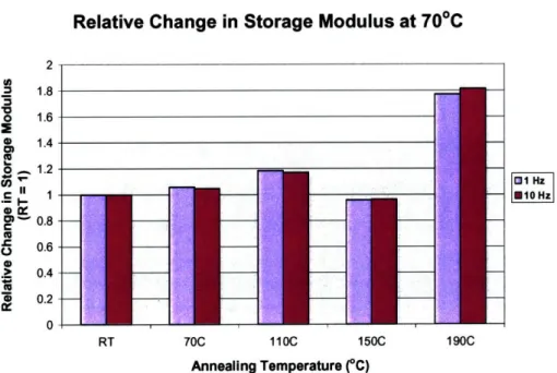
A similar trend is observed for storage modulus at 70'C. Figure 16 is a plot of

relative difference in storage modulus at 700_{C versus annealing temperature. Annealing}

the samples for one hour at a temperature up to 150TC does not affect the storage

modulus at 700_{C. However, at an annealing temperature of 190}0_{C, the storage modulus}

increases by as much as 80%.

Relative Change in Storage Modulus at 700_C

2 = 1.8 o 1.6 S 1.4 0) 0 1.2 c 1 I ,, 0.8 6 0.6 .> 0.4 0.2 0

1

-Hz ]

5101

Figure 16 - A plot ofrelative storage modulus at 700C versus annealing

temperature (RT = as-received).

The increase in storage modulus at an annealing temperature of 1900C can be

explained by the fact that the polymer chains begin to decompose, thus leaving the residual carbon atoms to form graphite fibers. Graphite fibers are known to have higher stiffness than polyurethane polymer chains. Thus after specimen is annealed at a temperature near its decomposition temperature, the storage modulus of the specimen increases [29].

The mobility of the macromolecular chains as indicated by the peak of the tan 6 curve increases slightly as the annealing temperature increases. Figure 17 is an overlay plot of the tan 8 curves.

C D (U

Temperatue (°C) vUws V3 S oTA Instummnts

Figure 17 -An overlay plot of the tan 5 curves from the DMA for samples annealed at different temperatures.

The glass transition temperature does not change significantly with the annealing temperature. Glass transition temperatures for all samples are roughly in the range of 300C ± 50C, as indicated by the peak of the loss modulus curve.

Pad softening during CMP could affect the CMP process and should be accounted for. As indicated by the DMA results, pad softening (a decrease in storage modulus) depends on the temperature to which the pad is heated during the CMP process. Additionally, specimens that are annealed at temperature above 1900_{C, close to the}

decomposition temperature of the material, exhibits a significant increase in storage modulus at 300_{C and 70}0_{C. Thus, if temperatures in the local area of contact between the}

pad and the wafer reach 190TC, significant changes in the properties of the CMP pad can adversely affect the planarity of the resultant wafers.

4.2.4 MDSC Results

Figure 18 shows a typical raw data output from the MDSC. The modulated DSC is able to separate heat flow into reversible and non-reversible components, as indicated by the curves show in blue and brown, respectively. The lines for each variable represent the two heating cycles of the MDSC experiment. Any chemical reactions that take place during the heating cycle will show up as a peak or valley on a heat flow curve. A peak on the heat flow curve represents an exothermic reaction, a reaction that releases heat into the surrounding. A valley on the heat flow curve indicates an endothermic reaction, a reaction that absorbs heat from its surrounding environment.

,105 - 000-0 005- .0,10- -0.15- -0.20---0.04 --0.06 -0.08 L -0.10 -0.12 -0.14 -,0 0 50 100 150 200 250

Em UP Temperature (*C) unliverm V3.5B TA Inhrumnets

Figure 18 - A typical raw data of the CMP soft padfrom the MDSC. Results from both heat cycles are shown. Curves shown in blue are the reversible heat flows; curves shown in brown are the

irreversible heat flows.

38

ii

I

Exo Up Temperature (*C) Universal V3.5B TA Instruments

Figure 19 - A typical raw data output from the first heat run ofMDSC. An irreversible endothermic

reaction can be observedfrom approximately 250

C to 1250 C.

From Figure 19, it can be seen that all reactions occur during the first heating cycle. A valley is observed in the temperature range of 300C to 90'C on the heat flow curve. This valley corresponds directly to one occurring in the same region on the irreversible heat flow curve. Since the reversible heat flow curve is relatively linear, it can be concluded that the reaction(s) occurring are irreversible. The heat of reaction of the process is determined by integrating the area over the valley. Figure 20 is a plot of the heat of reaction for different annealing temperatures. No noticeable correlation can be drawn between the heat of reaction and the annealing temperature. Thus, annealing the pads at high temperatures does not introduce additional reactions to the pad.

-002 0 l- 01-L_ -0 15 -0 20 --0.04 --0.06 -- 0.08 U.l --0.10 --0.12 --0.14 q j !))) I

Irreversible Heat of Reaction vs. Annealing Temperature '6-0 •4-e3 .0 2 "A RT 70"C 110*C 150°C 190oC

Annealing Temperature (oC)

Figure 20 - A plot of irreversible heat of reaction versus annealing temperature. No direct

correlation can be observed. (RT = as-received)

4.3 Soak Test

4.3.1 Diffusion Analysis

Diffusion in polymers is normally characterized by Fickian type diffusion [30]. For Dt/t2 < 0.4, general Fickian equation simplifies to Equation (7):

W =WM[C4

)J(Dt

(7)

where W is the current weight gain, Wm is the weight gain at saturation, D is diffusivity, d is the specimen thickness, and t is the diffusion time. For Dt/ d2 _{> 0.4, the general}

equation transforms to Equation (8)

W = We 1- exp ( Dr2 (8)

Equations (7) and (8) describe the linear and plateau portions of a plot of weight gain versus square root of time, respectively.

I

t

However, diffusion of both DIW and slurry into the soft pad do not exhibit the plateau part described by Eq. (8), as shown in Figure 21.

2 Z 1.8 1.6

6

Figure 21 -Plot ofweight percent gain versus the square root ofsoak time. The dotted line shown in

green represents a typical Fickian difusion.

Using Eq. (7), the coefficients of diffusion were calculated and are on the order of

lx10-6cm2/sec. Comparing these values to the diffusivity of polyurethane based hard

pads, which is lx107cm2/sec, the value of D in the soft pad is an order of magnitude higher [29].

In order to explain this phenomenon, a cross-section of a soft polymer pad was analyzed under SEM. It can be seen from Figure 22a and Figure 22b that the soft pad has a highly porous multilayer structure. The cross-section can be roughly divided into three layers. The top layer is made up of large non-uniform pores. The middle layer appears to be solid, while the bottom layer contains small non-uniform pores. It is likely that the pores trap water/slurry molecules in their cavities, thus liquid absorption is dominated by

fast filling of the cavities. As a result, the Fickian diffusion model is not applicable in describing liquid absorption into the soft pads.

Schematic Representation SEM

(a)

(b)

Figure 22 -a) A schematic representation of the cross section ofa soft CMP pad. The diagram depicts water molecules fast filling the cavities/pores in the top layer of the CMP pad. b) A SEM image ofthe cross-section.

Three distinguishable regions are observed.

The picture from the SEM also indicates that the polyurethane based pad belongs to the class of high density flexible foam. This is based on the fact that the pad is highly flexible and contains pores that are only visible under the microscope.

4.3.2 Effect of Slurry

4.3.2.1 TGA Results

Figure 23 is an overlay plot of the TGA raw data for all time intervals. It can be seen that the decomposition temperature is approximately 260'C and is not significantly affected by soak time of up to two months in slurry.

wate

moleci

50 100 150 200 250 300 350

Temperature (*C) urvvws V3 5B TA Insrments

Figure 23 -An overlay plot of the TGA raw data for all soak time intervals in slurry. Decomposition

temperature is designated as the onset ofsignificant weight percentage change (>10%).

4.3.2.2 TMA Results

Figure 24 is an overlay plot of the TMA raw data for all time intervals. It can be seen that the "shoulder" region (-900_{C to 125}0_{C), where the CTE increases followed by a} sudden decline, decreases as soak time increases.

-50 0VC)

Tenmerature (°C)

100 10 200

Univerd V3.SB TA In••nents

Figure 24 - An overlay plot of raw data for all soak time intervals from the TMA. I Day 3 3Day I Wk 4:- 'WKS AR I Day - 3 Days 1 Wk 2 Moe -200" 80 A•

At a soak time of one week, the "shoulder" region disappears. For soak time of two or more weeks, the "shoulder" region is replaced by a dramatic drop in CTE. One possible explanation for this phenomenon is that the chemicals in the slurry introduce

additional cross-links to the polymer chains. As soak time increases, more time is given for the cross-linking reactions to take place. Cross-links reduce the molecular motion of the chains and thus, reducing the specific volume of a polymer [25]. Therefore, for

specimens that have been soaked in slurry for an extended period, CTE is completely negative (shrinkage) in the "shoulder" region (-90'C to 1250_C).

Results from TMA indicate that large transverse shrinkage of pad occurs at lower temperatures with increase in soak time. Thus, the stable operating temperature range of the pad also decreases with soak time.

4.3.2.3 DMA Results

DMA tests are conducted with as-received non-soaked specimens and specimens soaked in slurry as describe in Section 3. For as-received pads and pads soaked in slurry, storage modulus decreases by approximately 50% within the pad operating temperature range.

Figure 25 is a plot of the storage modulus at 30°C for samples soaked in slurry for all time intervals. There is a general increase in storage modulus for up to two weeks. At two weeks, the storage modulus reaches a maximum. A slight decline in modulus occurs with soak time longer than two weeks.

Storage Modulus @ 30°C 01 Hz 010 Hz 0100 Hz RT 1 Day 3 1 Wk 2 4 2 Days Wks Wks Mos Soak Time

Figure 25 -A plot ofstorage modulus at 300

C versus soak time in slurry. Moduli were determined from the DMA at testing frequencies of 1Hz, O10Hz, 100Hz. (RT = as-received)

Storage Modulus at 700C

01Hz

lO °Hz

0100 Hz

RT 1 3 1 Wk 2 4 2

Day Days Wks Wks Mos

Soak Time

Figure 26 - A plot ofstorage modulus at 700C versus soak time in slurry. Moduli were

determined from the DMA at testing frequencies of 1Hz, 10Hz, 100Hz. (RT = as-received).

Figure 26 is a plot of the storage modulus at 700C for samples soaked in slurry for all time intervals. A similar trend is observed at 700_{C. There is a general increase in}

storage modulus up to two weeks followed by a slight decline in modulus after four weeks.

Figure 27 is an overlay plot of the tan 8 curves, also known as the damping curves, for all time intervals. It can be seen that the height of the peak of the tan 6 curve, which directly corresponds to the mobility of the macromolecular chains, decreases as soak time increases.

Cu

Temperattre (*C) UNvrsa V3 58 TA Intrumaets

Figure 27 -An overlay plot of the tan 6 curves for samples soaked in slurry for diferent time interv

The general increase in storage modulus for up to two weeks followed by a decrease in storage modulus can be explained by the fact that two competing processes, related to polymer cross-linking and plastisizing, respectively, occur at the same time. Cross-linking mechanism is confirmed by the decrease in the heights of the damping peaks, tan 8, shown in Figure 27. Decrease in the height of the tan 8 peak is related to decreased mobility of macromolecular chains/segments, and can be caused by cross-linking of macromolecules [30]. It is likely that competing plastisizing and cross-cross-linking

als.

processes are taking place within different layers of the multilayer soft pads. However, further structural analyses are required to establish the nature of these processes.

4.3.2.4 MDSC Results

Observed in MDSC, reversing endo- or exothermic heats can be associated with such thermodynamic reversible processes as vitrification, melting, and for some cases, crystallization [31]. These processes are typical for thermoplastic polymers. However, no reversible heat peaks after pad exposure to slurry are observed on the MDSC output as

shown in Figure 28. As such the tested pad does not belong to the class of

thermoplastics. An irreversible endothermic reaction is clearly observed for soft pad in temperature range of 25oC to approximately 125oC (first heat). The irreversible nature of the endothermic peak is confirmed using a second, repeated heat of the same sample. Absence of the heat peak during the second heat implies that all irreversible reactions have been completed during the first heat.

0 2 0. 3 -0.10 --0.12 --014 -0.16 -0.18 -50 50 0 100 150 200 250

Exo Up Temperature (C) Univer•al V3.5B TA Instrument

Figure 28 -A typical raw data output from the first heat run ofMDSC. An irreversible endothermic reaction can be observed from approximately 250C to 1250C.

For pad soaked in slurry, endothermic heat generally increases as soak time increases. It reaches a maximum after two weeks of exposure, as shown in Figure 29. This phenomenon can be explained by the hypothesis that slurry initiates a reaction that reaches maximum intensity after two weeks of soak. This soak time coincides with the soak time corresponding to the maximum values of storage modulus measured using the

DMA, as shown in Figure 24 and 25. Therefore, this endothermic reaction is possibly

associated with cross-linking or entanglements of the macromolecules within the polymeric soft pad.

48

0.1-z