Distribution of olivine and pyroxene in S-type asteroids throughout the inner main belt

Distribution of olivine and pyroxene in S-type asteroids

throughout the inner main belt

by

Shaye Perry Storm

Submitted to the Department of Earth, Atmospheric, and Planetary Sciences in Partial Fulfillment of the Requirements for the Degree of

Bachelor of Science in Earth, Atmospheric, and Planetary Sciences at the Massachusetts Institute of Technology

May 5, 2008 _L~A~Z

C 2008 Shaye P. Storm. All rights reserved.

The author hereby grants to M.I.T. permission to reproduce and distribute publicly paper and electronic copies of this thesis and to grant others the right

to do so.

Author

Department of Earth, Atmospheric, and Planetary Sciences May 5, 2008

Certified by

Signature redacted

Professor Richard P. Binzel Thesis Supervisor

Signature redacted

Pressor Sam Bowering Chair, Committee on Undergraduate Program The author hereby grants to MIT permission to reproduce and to distribute pubiy paper and

electronic copies of tis thesis document in whole or in part in any medium now known or hereafter created.

bMN5 UTE T HN 'Q 9Y

OCT

2 4 2017

LIBRARIES

MiTLibraries

77 Massachusetts Avenue

Cambridge, MA 02139 http://Iibraries.mit.edu/ask

DISCLAIMER NOTICE

Due to the condition of the original material, there are unavoidable flaws in this reproduction. We have made every effort possible to provide you with the best copy available.

Thank you.

This thesis was submitted to the Institute Archives without all the required signatures.

Distribution of olivine and pyroxene in S-type asteroids throughout the inner main belt

By

Shaye P. Storm

Submitted to the

Department of Earth, Atmospheric, and Planetary Sciences

May 5, 2008

In Partial Fulfillment of the Requirements for the Degree of Bachelor of Science in Earth, Atmospheric, and Planetary Sciences

ABSTRACT

The mineralogical composition of asteroids can be constrained using visible and near-infrared (VNIR) spectroscopy. The most prominent spectral features observed over this wavelength range are due to olivine and pyroxene, the two most abundant minerals in both chondritic and achondritic meteorites. The observed ratio of these two minerals is highly dependent on the amount of heating that an asteroid has undergone. The 1-micron band center wavelength and the band area ratio (BAR) between the 2- and 1-micron bands reveal relative abundances of olivine and/or pyroxene on an asteroid surface (Gaffey, 1993). A large sample of S-, A-, V-, and R-type asteroid spectra was collected over the visible and near-IR wavelengths during the second phase of the Small Main-belt Asteroid Spectroscopic Survey (Bus and Binzel, 2002) and using the low-resolution SpeX spectrograph (Rayner, 2003) at NASA's Infrared Telescope Facility (IRTF).

Here we present a methodology for calculating the location of the 1-micron band center wavelength and BAR with appropriate 1- sigma uncertainties. This method was used to characterize 188 S-type asteroids throughout the inner main belt. We will also present the distribution of olivine / pyroxene throughout the main belt by measuring how the S-type mineralogy varies with heliocentric distance. This will provide a better understanding of both the thermal processing across the main belt and subsequent mixing of asteroids through collisional and dynamical processes. Thesis Supervisor: Schelte J. Bus

Title: Support Astronomer, University of Hawaii Thesis Supervisor: Richard P. Binzel

Acknowledgments

The work in this thesis has been a joint effort between myself, Schelte "Bobby" Bus of the Institute for Astronomy at the University of Hawaii, and MIT Professor of

Planetary Science, Richard Binzel. I want to thank Bobby for giving me the opportunity to work on this great project and join him in Hawaii for a summer. I want to thank Rick for his constant guidance and advice at MIT. I also want to thank Francesca DeMeo and Cristina Thomas for being great lab mates and advisors, and Mary Masterman for being a great UROP and physics classmate.

I want to thank my family for always supporting me at MIT and beyond, and for

reading this thesis. Finally, I want to thank my friends for making MIT the best place to be.

Contents

Chapter 1: Introduction... 6

1.1 Structure and Evolution of the M ain Belt ... 6

1.2 M ineralogy of S-type Asteroids ... 8

1.3 S-type Spectra ... 11

1.4 Laboratory Calibrations of Olivine and Pyroxene M ixtures...12

Chapter 2: Analysis of VNIR Spectra... 15

2.1 Observations and Asteroid Sample ... 15

2.2 Data Reduction ... 16

2.3 Improvement of uncertainty estimates ... 16

2.4 W riting a program to calculate BAR and BICW ... 19

2.5 Calculation of Band Area Ratio... 19

2.6 Calculation of Band I Center W avelength... 21

Chapter 3: Results ... 24

3.1 Performance of IDL program ... 24

3.2 M ixing Line Distributions ... 25

3.3 Heliocentric Distance Distributions ... 25

Chapter 4: Discussion ... 29

4.1 Heliocentric trends...29

4.2 M ixing line features... 30

4.3 Discussion of IDL program... 31

4.4 Future work ... 32

R eferen ces ... 3 3 Appendix A: Table of Asteroid Properties ... 34

Appendix B: IDL Program to analyze S-type VNIR spectra... 39

List of Figures and Tables

Structure of the m ain belt ... 8

Basic structure of differentiated asteroid ... 10

S-type spectral characteristics... 12

M ixing line calibrations ... 13

Uncertainty estimate correction ... 18

Continuum fits to spectrum ... 20

Fitting B and I ... 23

Mixing line plot for all asteroids ... 26

Heliocentric distribution for all asteroids ... 27

Running box car average of heliocentric distribution ... 28

S-type subgroup classification ... 31

Mixing line plot of S-type families and background asteroids ... 50

Heliocentric distribution of S-type families and background asteroids .. 51

Heliocentric distribution of S-types with diameters > 50 km... 52

Heliocentric distribution of S-types with diameters < 50 km ... 53

Table 1: Calculating BICW ... 22

Table 2: Success Rate of Program ... 24

Chapter 1: Introduction

In this thesis, I describe the results of a spectroscopic survey of inner main-belt asteroids, with a focus on S-types. Chapter 1 contains relevant background

information on the structure and thermal evolution of the main belt, the mineralogy of S-type asteroids, and previous laboratory calibrations of olivine and pyroxene spectra. Chapter 2 discusses telescope observations, and methods for determining the relative abundance of olivine and pyroxene in S-type asteroids. Chapter 3 describes the results developed from the previous chapters. Chapter 4 contains discussions of the results.

1.1

Structure and Evolution of the Main Belt

The asteroid belt contains important clues about the primordial chemistry and thermal processing of materials in that region of the solar system as a function of distance from the sun (Bell et aL., 1989). The asteroids that currently comprise the main belt are believed to represent the conditions in which they formed (Gradie,

1982). Although it is unclear how much dynamical processing has affected the

original structure of the belt, it has been a goal to map the material structure of the asteroids throughout the main belt and look for current compositional trends that could explain early formation. A general theory of the stratigraphy of the main belt was presented in Asteroids H(Bell et aL, 1989). Figure 1-1(b) shows the general thermal trend of the main belt, and the paper stated that "the igneous types dominate

the belt sunward of 2.7 AU ... [and] the heating mechanism which metamorphosed

the chondrites and melted the achondrites was one which rapidly declined in efficiency with solar distance." Fig 1-1(a) shows the general taxonomic structure of the main belt as it was known at the time.

Although we will not argue with the broad structure stretching from 2.0 - 5.0 AU that places igneous material closer to the sun and primitive material further away,

we believe that there may be small-scale structure in the inner main belt that has not been fully studied due to limitations on the number of asteroids observed and the quality of the data obtained. If we can show that there is, or that there is not, small-scale structure in the inner main belt, it will help us understand the original heating mechanisms of the main belt.

There is still large debate within the community about the large scale heating processes of asteroids in the main belt. Several accretion and heating models were discussed in Asteroids IHin the chapter titled "Thermal Evolution Models of

Asteroids." I will only briefly discuss the basic ideas of the most popular models, and the reader should refer to that chapter for a more in depth discussion.

If the primary heating of asteroids was supplied by the magnetic field of the T-tauri Sun, then it would be expected for heating trends to be uniform and follow a simple heliocentric trend that places the most thermally altered rocks closer to the sun. In addition to the possibility of magnetic heating, it is believed that

aluminum-26 (26_{Al) was another major contributor to asteroid heating. The amount of} 26_A1

remaining in an asteroid after accretion is dependent on the time of accretion; less

2 6_{A1 is available to be incorporated into a body the longer it takes to accrete}

(McSween, 2002). Asteroid accretion time increases with increasing distance from the sun, so asteroids that formed further out in the main belt had less 26_{AI after}

accretion. A heliocentric composition gradient should thus be formed, but irregularities are possible if the 26Al distribution was inhomogeneous.

This study aims to advance the understanding of these thermal processes by looking for detailed mineralogical trends from 2.0 to 3.0 AU using the most recent visible and near-infrared spectroscopic survey data for over 200 asteroids. If

.I

taxonomic class in the inner main belt, it may provide a better understanding of both the early thermal processing across the main belt and subsequent mixing of asteroids through collisional and dynamical processes.

1.0 0.5 uJ

z

z

Figure 1-1. Distribution (taxonomic, a; thermal, b) of the asteroid belt shown as relative abundance as function of distance from sun (taken from Bell et al, 1989). We will attempt to

refine this overall theory and look for small-scale structure in the inner main belt among S-type asteroids.

1.2 Mineralogy of S-type Asteroids

The thermal history of asteroids can be inferred from their current

mineralogical properties. However, available technologies make direct samples of asteroids difficult and expensive to obtain. The most widely available physical samples of asteroids on Earth come from meteorites, which are pieces of planets or small bodies in the Solar System that fall to Earth. Since they were once part of larger

parent bodies, meteorites provide us with direct evidence to understand asteroid mineralogy. Although this can provide great insight into the physical nature of asteroids, it is still generally unknown which specific asteroids supplied any given meteorites, and the relatively small number of parent bodies does not provide a large enough sample of asteroids. Remote sensing is still the best widely available analysis technique for studying the physical nature of large numbers of small bodies in the Solar System.

The mineralogy of S-type asteroids is dominated by olivine and pyroxene, both silicate minerals found throughout the Solar System. Olivine has a chemical formula of (Mg, Fe)2SiO4. There are several chemical forms of pryoxene, but a general

chemical formula for orthopyroxenes is (Mg, Fe)SiO3. The S-type taxonomic classification we use here is based on the Tholen taxonomy (Tholen, 1989). More updated taxonomies have been published with more refined subgroups of S-types (Bus

and Binzel, 2002b), but the more detailed taxonomic classification of specific asteroids is not immediately necessary for this general analysis of silicate rich asteroids.

The importance of the relative abundance of olivine and pyroxene in S-types in relation to thermal trends can be best understood by looking at the range of heating that occurred in the main belt. In the outer main belt, C-type asteroids, which provide the Earth with carbonaceous chondrite (CC) meteorites, have

undergone little to no heating. CCs have the chemical composition of the primordial solar nebula, and contain the solar abundance level of elements in atomic form. When enough heat is added to a CC, molecules begin to form and some pyroxene,

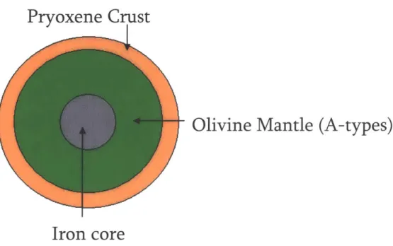
olivine, and metallic iron is produced. With more heating, olivine, pyroxene, and metallic iron increase in abundance again, with olivine being the most represented. S-type asteroids are thought to represent these previous two stages of heating. If there is further heating, differentiation will occur; an iron core will sink to the center, a pryoxene crust will rise to the surface, and an olivine mantle will settle in the

___________ ________ -- - - - -I

middle. This layer distribution is due to the weight of the minerals, and a very basic picture of this, shown in Figure 1-2, can be thought of as a V-type asteroid, such as Vesta.

Pryoxene Crust

Olivine Mantle (A-types)

Iron core

Figure 1-2. The basic structure of a differentiated asteroid, such as Vesta. With a lot of heating, a metallic iron core will sink to the center, a pyroxene crust will rise to the surface, and an olivine mantle will settle in the middle.

As mentioned previously, S-type asteroids were formed in between the stages of no heating (C-types), and the most heating (V-types). The S-types that were heated just above C-types are believed to contain a fairly even mix of olivine and pyroxene, while the S-types that were heated even more, but not to full

differentiation, are believed to contain a higher abundance of olivine than pyroxene. Therefore, it is important to determine the relative abundance of the two minerals in an asteroid to understand how much heating it has undergone.

1.3 S-type Spectra

It is possible to determine the relative abundance of olivine and pyroxene in an asteroid because the minerals control the observed spectral features of silicate-rich asteroids (Gaffey, 2002). With any reflectance spectrum, the chemistry of the

material reflecting sunlight will determine what wavelengths of light get absorbed or reflected. Since pyroxene has absorption features located around 1- and 2-pm, and olivine has absorption features located around 1-pm, remote sensing of asteroids with spectrometers sensitive to NIR wavelengths allows the study of these important minerals. These two broad absorption features are composed of higher resolution bands and are controlled by the physical structure of the mineral, and by the vacancies in the silicon-oxygen crystal structure. Fe+ and Mg+ are the primary ions that fill in the olivine vacancies, where Fe+, Mg+ and Ca+ fill in the pyroxene

vacancies. Current work being done by Sunshine et a]. (2007) uses Modified Gaussian

Modeling (MGM) to attempt a deconvolution of the broad spectral features into the higher resolution bands controlled by the mineral vacancies. Our study focuses on the lower resolution, broad 1- and 2-pm bands.

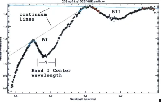
To better describe these bands, Figure 1-3 is a labeled snapshot from our computational analysis that shows the VNIR spectrum of asteroid 278 Paulina. Relative reflectance, which represents relative photon counts from the observed asteroid, is plotted as a function of wavelength. The 1- and 2-Pm bands mentioned above are shown as BI and BII, respectively. The Band I Center wavelength (BICW) label shows an approximation of where the center of BI might be. The calculation of this wavelength value with appropriate uncertainty values for our sample of S-type spectra is the focus of this study. The blue and red lines are approximations of the spectral continuum. Details on the calculation of the continuum, the band areas, and the BICW will follow in the methods section.

278.sp14.o1 033.VNIR.smth.m BII 1A continuum lines jI.3_1.BI Band I Center o.9 wavelength OA 0.5 1.0 1.5 2.0 Wmveuesgth (rnloroa)

Figure 1-3. Identification of important features of an S-type asteroid spectrum that will be used in this study. We developed methods to define the continuum lines, and calculate the Band I (BI) and Band II (BII) areas, and the Band I Center wavelength.

1.4 Laboratory Calibrations of Olivine and Pyroxene Mixtures

The foundational work in laboratory calibrations of olivine and pyroxene spectral properties was created and published by Edward Cloutis and Michael Gaffey

(1986) whose spectra were acquired for pure end members of olivine and pyroxene, as

well as for varying mixtures in between. They used the spectra to determine the calibrations that would be most useful for inferring the physical properties of asteroids through remote reflectance spectroscopy. The band area ratio (BAR) and the BICW (to be explained in greater detail in methods section) were two calibrations that were deemed useful for determining the relative abundances of olivine and pyroxene. A 'mixing line' was created by plotting BAR as a function of BICW. It represented how the two calibrations behaved in relation to one another as the mixture proportions of olivine and pyroxene varied. The line is a useful tool for the

study the olivine / pyroxene abundance ratio in meteorites and asteroids (see Figure 1-4). If the BAR and BICW can be calculated for a newly discovered body, they can be plotted on the line and can give an approximation of the relative olivine /

pyroxene abundance.

11. 10 Oft

KEY

0 90- 125 mier ons, wet &ioved 0 63-SO microne. wet sieved 0 38-83 microns, wet sieved

3 1.05 I g 8 X 63-00 microns. dry sieved

E C 1.00 C 0.95 E100 0.90 0.0 0.2 0.4 0.8 0.8 1.0 Pyx/ (Pyx+Olv)

Figure 1-4. Mixing line developed by analysis of laboratory spectra of olivine and pyroxene end-members and different olivine-pyroxene mixtures (taken from Cloutis and Gaffey, 1986). The mixing line is a calibration that uses the Band I center wavelength and the Band Area Ratio to analyze the relative abundance of olivine / pyroxene in a meteorite or an asteroid spectrum. We will calculate these two values for our asteroid sample and see how the asteroids plot on the mixing line.

We hope to understand the distribution of our asteroid data set on this mixing line. Previous studies have found that most asteroids do fall somewhere along this mixing line with a location dependent on their olivine / pyroxene abundances. Meteorites, on the other hand, have been found to plot off of the line much more frequently. This is not currently understood and is outside the range of this paper. It is important to note that the mixing line is not absolutely controlled. There are other factors, such as grain size and type of pyroxene (low calcium pyroxene vs. high calcium pyroxene), which will shift the mixing slightly up or down. So the mixing line is more like a "mixing range".

The technical goal of this research is to create a program that will calculate the BAR and BICW consistently for all S-type spectra with minimal user input, in

addition to calculating appropriate 1-sigma uncertainties for the BAR and BICW. Previous studies that have calculated these spectral properties have lacked the rigor to make the calculations unbiased to user input and produce repeatable uncertainties within reason.

One of the scientific goals of this study is to plot all of our observed asteroids as a function of BAR versus BICW and see where they plot along the mixing line. Although we are initially lumping all of the S-types into a single classification, we are also interested to see if there are any distinct patterns formed along the mixing line that could represent distinct grouping among the S-types to show smaller groups within the larger classification. The Bus classification (2002b) breaks the S-types into several smaller groups, and (Gaffey, 1993) identifies seven possible S-type subgroups. The main scientific goal of this research is to look for heliocentric trends in thermal processing among the S-types. For our wavelength range and data quality, the most useful calibration for the relative abundance of olivine / pyroxene is the BICW. This is because BI is affected by both olivine and pyroxene. The relative abundance of the two minerals will control the location of the band center. We will conclude with plots of BICW as a function of heliocentric distance and see if there is any structure in the inner main belt S-type population.

Chapter 2: Analysis of VNIR Spectra

2.1 Observations and Asteroid Sample

The spectra used in this study were obtained in the visible wavelengths from Phase II of the Small Main-Belt Spectroscopic Survey (SMASSII) (Bus and Binzel, 2002a). SMASSII used the 2.4-m Hiltner and 1.3-m McGraw Hill telescopes on Kitt Peak and had a wavelength range of 0.435-0.925pm. Near-infrared data were

obtained from continued runs on NASA's Infrared Telescope Facility using a low-to-medium resolution spectrograph and imager called SpeX (Rayner, 2003). We used SpeX to observe with a wavelength range of 0.7-2.49 pm. The SpeX data were crucial for this study, since they included the 1- and 2-jm bands which are diagnostic of the olivine and pyroxene mineral chemistry of the asteroids in this study.

In total, we analyzed 188 S-type, 12 V-type, 9 A-type, and 2 R-type spectra. The main goal of this study was to analyze the S-type asteroids. The other taxonomic classes were useful, especially known pyroxene-rich V-types, for a check on the analysis. Additionally, taxonomic classifications tend to be amorphous in many cases. Some asteroids classified as R-type might be closer to S-type, and vice versa. But for simplicity, we only used S-type classified asteroids in the final analysis of heliocentric trends.

It is important to note that these 211 asteroids are not a random sample of the inner main belt. Most of them were observed with an observational bias towards asteroids in families. Therefore, we have a lot of asteroids that might be

representative of the same parent body. This will be taken into account in the final analysis where family members will be averaged together into a single data point.

2.2 Data Reduction

We reduced the raw reflectance spectra using standard Image Reduction and Analysis Facility (IRAF) and Interactive Data Language (IDL) procedures. Pixel-to-pixel variation and thermal noise were removed. Pixel values were converted to wavelength values using a manual calibration technique with an argon lamp spectrum. Individual exposures of the same asteroids spectrum were stacked to increase the signal-to-noise ratio and they were normalized using observed standard star spectra. The NIR water lines were removed by using an atmospheric

transmission model developed for Mauna Kea to fit the spectra.

The final spectral reflectance data used in this study for each asteroid ranged from 0.435 pm to 2.49 pm. Each spectral data point had a 1-sigma uncertainty associated with it. Our method of calculating a BICW directly made use of these uncertainties, so we gave them close attention at the start.

2.3 Improvement of uncertainty estimates

We sought to adjust the uncertainty values to provide a more realistic representation of the error at each wavelength. The initial 1-sigma uncertainty assigned to each data point of the S-type spectra represented random photon counting statistics that were mainly associated with the SpeX detector for the NIR wavelengths

(Bus and Binzel 2002), or that were associated with the visible detectors on the Hiltner and McGraw Hill telescopes for the visible wavelengths.

The adjustment was aimed to reflect the systematic errors introduced to the final spectra through the telluric correction, which accounts for water in the Earth's atmosphere and removes the NIR water lines by fitting an atmospheric transmission model developed for Mauna Kea to the spectra. The model fitting is never perfect,

and we believe that the model's disproportionate affects for all wavelengths are a source of systematic error.

To improve the uncertainty values, we spline fit 400 asteroid VNIR spectra using an IDL program written by Eric Volquardsen of the University of Hawaii. Spline fitting approximates a curve as a piecewise polynomial function. We effectively smoothed the spectra by representing their complex structure as a combination of simple polynomials. For each wavelength channel, we recorded 6,

which was the difference between the spline fit reflectance (sfr) and the observed reflectance (obsr), divided by the original 1-sigma uncertainty (osig):

1 = (sfr -obsr) / osig

We then found the mean, rq, and standard deviation, o; of 5 across 400

asteroids for each wavelength channel. q and -were summed in quadrature to obtain final uncertainty correction values for each channel, p, which are plotted in Fig 2-1.

p =(r +oF1 2

The original 1-sigma uncertainties for each data point were multiplied by the appropriate p value to obtain improved uncertainties, p'

p'= osig* p

The visible wavelength channels had the highest p values and were in the most need of systematic correction. This was expected because the visible SMASS II data had lower photon counts and lower signal-to-noise than the NIR SpeX data. It was also not surprising that the NIR wavelength channels near 1.4pm were in need of more systematic correction than other NIR wavelength regions, due to strong

atmospheric absorption bands in that region. Note that some wavelength channels had p values that were below 1.0, indicating that the 1-sigma uncertainty should be reduced.

5.0 4.5 0 0 0 4.0 0 Go 0 3.5 -00 o 0 o

S

0.0

Figure 2-1. This plot represents the correction multiplier to the 1-sigma uncertainty for each wavelength channel. See the preceding text for a detailed explanation of the definition of the uncertainty correction.

2.4 Writing a program to calculate BAR and BICW

Having improved the uncertainty estimates for each wavelength channel, we were confident that the uncertainties of each spectral data point were more accurate representations of the uncertainty at each wavelength and could be used to calculate the BICW and BAR. However, several calculations and manipulations had to be performed on the spectra before anything could be done to calculate those values.

To automate these calculations and manipulations, we wrote a program in Interactive Data Language (IDL). As mentioned in the opening, the goals of this program were to remove as much user input as possible, while making the program respond uniformly to all ranges of S-type (and similar taxonomic type) spectra. The only user inputs were wavelength ranges of the two relative maxima and two relative minima of the spectrum.

The important details of the program pertaining to BICW, BAR, and the calculations of uncertainty and the reasoning behind them will be summarized in the following sections, and the entire IDL program is included as Appendix B.

2.5 Calculation of Band Area Ratio

The BAR was one of the calibrations deemed useful for understanding the relative abundance of olivine / pyroxene in an asteroid. This makes sense, since only pyroxene has an absorption feature at 2-pm. If there is little to no pyroxene in an asteroid, then the BII area will be small, making the BAR very small.

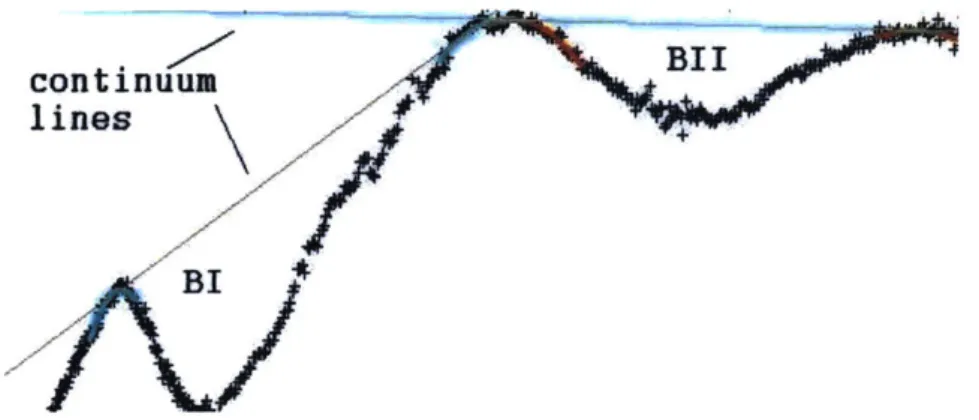
To calculate the BI and BII areas, continuum lines for each absorption band had to be defined. To do this, we fit quadratic polynomials to the local maxima

polynomials were connected by a line that was tangent to both, and this line was defined as the continuum of the band (shown as colored lines below).

BII

continuum lines

BI

Figure 2-2. Illustration of the IDL program fitting local maxima (seen as colored curves) and continuum lines (seen as colored lines) on an S-type spectrum.

The calculation of the continuum bands for BI and BII was the first step to calculate the BAR. Next, we had to settle on a definition of band area. The definitions of BI and BII were presented by Cloutis et al (1986) in his calibration

paper:

"The band I area is defined as the area enclosed by the spectral curve and a straight-line tangent to the relative maxima at 0.7 and 1.4-1.7 pm. The band II area is enclosed

by the spectral curve and straight line fixed on the curve at 2.4 Pm (because the

absorption wing is incomplete) and the 1.4- to 1.7-pm maximum."

This traditional BAR definition was used with two slight modifications. First, it was not possible to determine the exact continuum lines to the spectral curve for both band areas; fitting a line to the local maxima of the spectra was not the most accurate definition of the continuum line. We instead used the method described earlier. This gave a more robust approximation for the continuum, which was also important for calculating the BICW. Second, not all BII areas were cut off at 2.5pm. We fit a second order polynomial to the end of the spectrum to determine the curvature of the spectrum in that wavelength region. If the spectrum had a relative maximum in the

2-2.5pm region, then the BII area was measured up to that maximum wavelength instead of 2.5 m.

Once we defined our BI and BII areas, we calculated the areas with the trapezoid approximation. The exact calculation of BAR and associated uncertainty can be read in Appendix B.

2.6 Calculation of Band I Center Wavelength

The calculation of the BICW began by dividing out the continuum for BI. This continuum slope varies among asteroid spectra. Laboratory spectra of olivine / pyroxene mixtures, however, do not show any slope in the reflectance spectra. Therefore, to use the calibrations presented by Cloutis (1986), it was necessary to normalize Band I. The cause of the varying spectral slope is not currently understood and is subject of separate research.

At this point of the study, the most subjectivity entered the calculations. Calculating and defining the BICW was a difficult task because the definition of the band center contained a lot of subjectivity. It was important to remember that BI was a convolution of absorption bands arising from distinct ion vacancies for olivine and pyroxene. The complexity of the band created the difficulty of defining a band center when only looking at the convolved band. It was generally agreed that the absolute band minimum, attained from a high order polynomial fit, was not the desired feature. The broadness of a second order polynomial suited BI for fitting since we were looking to track a broad structure. Once making this subjective choice of method, we applied it consistently. Thus, relative fits are expected to be robust.

After we made the choice of a quadratic polynomial fit, we tested which sections of the band to fit. It was clear that the bottom of BI often had a quadratic

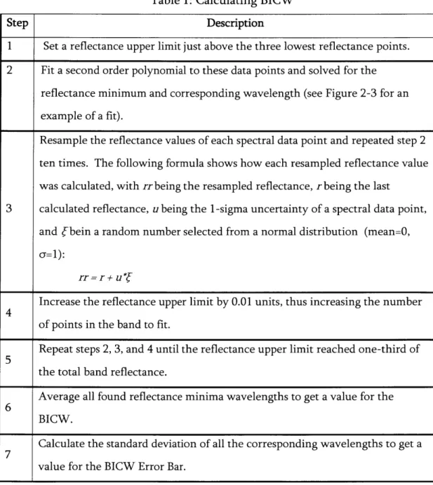
shape, but the rest of the band quickly diverged from quadratic to a higher order shape. Therefore, if the band was fit from small reflectance values all the way to the highest reflectance values, a lot of systematic error would be introduced. We found that fitting a second order polynomial over the bottom third of the band introduces little or no systematic error. After several trials with different fit parameters, the BICW was calculated in the following automated way as part of the larger IDL program (see the following Table).

Table 1: Calculating BICW

Step Description

1 Set a reflectance upper limit just above the three lowest reflectance points.

2 Fit a second order polynomial to these data points and solved for the

reflectance minimum and corresponding wavelength (see Figure 2-3 for an example of a fit).

Resample the reflectance values of each spectral data point and repeated step 2 ten times. The following formula shows how each resampled reflectance value was calculated, with rr being the resampled reflectance, r being the last

3 calculated reflectance, u being the 1-sigma uncertainty of a spectral data point,

and bein a random number selected from a normal distribution (mean=0,

c-=1):

rr =r + u

Increase the reflectance upper limit by 0.01 units, thus increasing the number 4

of points in the band to fit.

Repeat steps 2, 3, and 4 until the reflectance upper limit reached one-third of

5

the total band reflectance.

Average all found reflectance minima wavelengths to get a value for the

6

BICW.

Calculate the standard deviation of all the corresponding wavelengths to get a

7

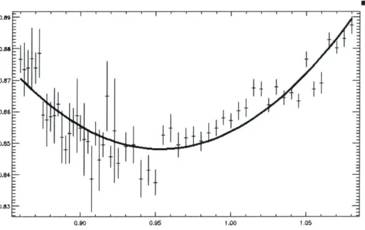
U-0-Ag 0.A& 0.87 0.86 0.85 0.84 a.90 f.00 I.05

Figure 2-3. A second order polynomial fit to data points of Band I. This is a snapshot from our IDL program in which we solved for the reflectance minimum and corresponding wavelength of Band I. The horizontal axis represents wavelength (microns), and the vertical axis represents relative reflectance.

t

t ttt

ttt

t

P"

16-7

Chapter 3: Results

3.1 Performance of IDL program

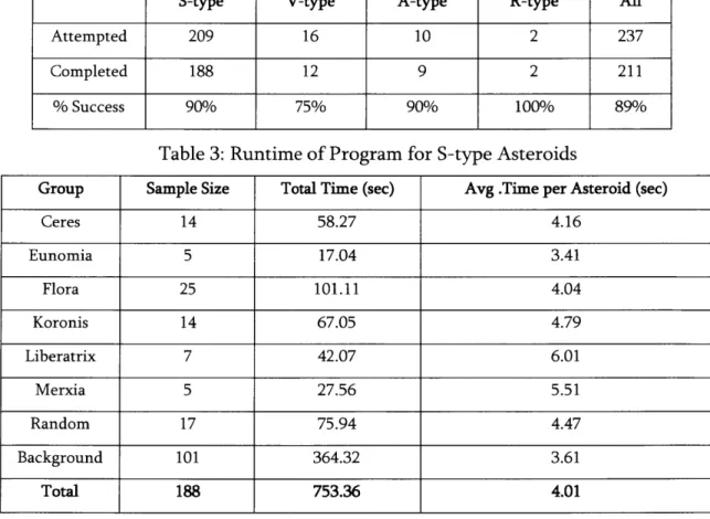
The IDL program was able to run to completion on 88% of the asteroids in an automated fashion. The time to process a single spectra averaged 4.01 seconds, and was most dependent on the depth of the absorption bands. The success rate and runtime statistics are shown in the tables below.

Table 2: Success Rate of Program

S-type V-type A-type R-type All

Attempted 209 16 10 2 237

Completed 188 12 9 2 211

% Success 90% 75% 90% 100% 89%

Table 3: Runtime of Program for S-type Asteroids

Group Sample Size Total Time (sec) Avg .Time per Asteroid (sec)

Ceres 14 58.27 4.16 Eunomia 5 17.04 3.41 Flora 25 101.11 4.04 Koronis 14 67.05 4.79 Liberatrix 7 42.07 6.01 Merxia 5 27.56 5.51 Random 17 75.94 4.47 Background 101 364.32 3.61 Total 188 753.36 4.01

After running our IDL code, we had calculated the BAR, BICW and associated 1-sigma uncertainties for each asteroid. The BICW uncertainty averaged 0.00664pm and had a range of 0.00087pm - 0.06184pm. A table with these numbers, along with

semimajor axes, families, and diameters can be found in Appendix A. Mixing line plots and heliocentric distribution plots will be shown in this chapter and in Appendix C.

3.2 Mixing Line Distributions

To see where our sample fell on the mixing line, we plotted the BICW as a function of BAR for each asteroid. As seen in Figure 3-1, most of the asteroids fell along or around the mixing line. The V-types, which represent the pyroxene rich Vestoids, plotted in the pyroxene rich region of mixing line. The A-types, which are a taxonomic class of olivine rich asteroids, are mostly found in the olivine rich region of the plot (several of the A-types plotted among the S-types). The S-types families and background asteroids are plotted along the mixing line in Figure C-1.

3.3 Heliocentric Distance Distributions

To look for any trends in the olivine / pyroxene abundance ratio, we plotted BICW as a function of semimajor axis (AU). Note that 3 of the 188 asteroids in our sample are at heliocentric distances that classify them as Near-Earth objects. These objects are shown in most of the heliocentric distributions, but not in Figure 3-3 to prevent a skewed average.

Figure 3-2 shows all of the asteroids in our sample. Figure C-3 specifically shows the S-type families and background asteroids. To correct for family bias and possibly bring out any trends not noticed in the whole dataset, we created plots of S-type asteroids less than 50 km and asteroids greater than 50 km, seen in Figures C-3 and C-4, respectively. We also performed a running-box car average with 10

asteroids represented in each data point, seen in Figure 3-3. Family members were averaged into 1 data point before overall averaging to correct for bias. The family data points were plotted with a size proportional to the number of family members represented. This is plot was the main focus of this study and will be discussed in the following chapter. 1.10 1.05 1.00 Pq 0.95 0.90 0.85 0.0 0.5 1.0 1.5 2.0 2.5 BAR

Figure 3-1. Mixing line plot for every asteroid in our sample. The mixing line was taken

from Cloutis (1986). The V-types plot at the pyroxene-rich end of the mixing line as

expected. Some of the A-types plot at the olivine-rich end of the mixing line as expected, while others plot among the S-types. Most of the S-types plot on or around the mixing line while forming two distinct clusters.

All Asteroids * S-type 0 R-type * A-type L V-type Mixing Line 'E -4 I T

-I

1.10 All Asteroids * S-type m R-type A V-type 1.05 0 A-type 1.00 0.95 0.90 0.85 0.80 1.1 1.6 2.1 2.6 3.1

Semimajor Axis (AU)

Figure 3-2. The Band I Center wavelength plotted as a function of semimajor axis (AU) for every asteroid in our sample. The S-types (in blue) are the focus of our study and will be plotted and analyzed alone in the following figures.

A A Running Box Car Average 1.05 0 Mean (N=10) A a Merxia(5) A A N Liberatrix(7) A W Koronis(14) A 0 Flora(25) * Eunomia(5) 1 A A |Ceres(14) A A A + Random A A Background

U

A

j

Semimajor Axis (AU)

Figure 3-3. A running boxcar average with ten asteroids represented in each data point (family members were averaged into 1 data point before overall averaging). The three NEAs in our sample were removed before averaging and are not shown in this plot. There appears to be a trend of decreasing olivine / pyroxene abundance ratio moving further away from the sun. This plot will be discussed in greater detail in the next chapter.

Chapter 4: Discussion

4.1 Heliocentric trends

The average appears to reveal a trend of decreasing olivine / pyroxene ratio moving further away from sun in the inner main-belt. Figure 3-3 showed the original S-type data with a running box-car average plotted over it. At the start of the main belt at around 2.0 AU, there is a dominance of S-types with a higher BICW,

indicating higher concentrations of olivine over pyroxene in the asteroids. The Flora family is the only family in our sample that is found in that region of the main belt and its averaged data point also plots at a high BICW. Moving to higher heliocentric distance, from around 2.0 AU to nearly 2.5 AU, there is a sharp drop in BICW as it shifts to lower wavelengths. This drop indicates a decrease in the amount of olivine in the olivine / pyroxene mixture of the S-types in that region of the main belt. From

2.5-2.9 AU, there is a gradual increase in BICW.

This plot could indicate several things, but there does appear to be a

mineralogical trend. If the trend is real, then it places more thermally altered S-types at lower heliocentric distances in the inner main belt. This agrees with the main belt heating theories, such as magnetic heating from the T-tauri Sun and radioactive decay heating from 26_{Al, that were discussed in the introduction.}

However, the trend we present in Figure 3-3 is not obvious, nor conclusive. It is also definitely not a smooth trend that can be fit with a simple linear or power function. More asteroids will be needed to fully understand the trend that we are starting to see, but for now we think we are seeing a higher concentration of olivine-rich S-types closer to the sun.

One possibility for the lack of a clear trend is that the original heliocentric distribution of the thermal structure of the main belt was disrupted by dynamical

mixing of the S-types. It is also possible that there is not a trend among the S-types in the inner main belt, and that the boxcar average is a false indicator.

4.2 Mixing line features

Figure 3-1 showed all of the asteroids in our study plotted over the mixing line. Although this research was primarily aimed at finding heliocentric trends, the mixing line plot showed some interesting features. The S-types exhibited clustering patterns on the mixing line. Gaffey et a]. (1993) analyzed 39 S-types and divided them into seven subgroups, one of which he hypothesized contained parent bodies for

OCs. That OC subgroup was represented on the mixing line as the S(IV) group seen in the figur below. On our plot, there are two distinct clusters of S-types centered on

0.98pm BICW - 0.4 BAR and on 0.92pm BICW -0.8 BAR. These clusters fall in or

near the Gaffey S(IV) subgroup and might represent the most OC-like asteroids in the main belt. There is still no clear answer for the OC parent-body question and S-type classification and understanding is still being formulated. The results in this study will hopefully add more data to the discussion. A discussion of S-types and their relation to OCs can be found in Asteroids hIin the chapter entitled: "Meteoritic Parent Bodies: Their Number and Identification."

1.10 S(I) F S 11) b. 1.00 S(SI) 1.00 -S IV) S(VI)-2 S(VII) - 0.95 -( C 0.90' 0.0 0.5 1.0 1.5 2.0 2.5 3.0 Band I I Band I Area Ratio

Figure 4-1. S-type subgroup classification taken from Gaffey etaL. (1993). We bring this figure to attention since the S-types in this study form distinct clusters when plotted on the mixing line axes that roughly coincide with the S(IV) classification seen above.

4.3 Discussion of IDL program

As mentioned in the results, our program ran with an 88% success rate. The spectra that experienced failure were often the ones with extremely noisy BII that caused one of the several fitting calculations to fail. The low quality of these spectra made them less than ideal for our study, so we found the failure acceptable, and at times, welcome.

With regard to runtime, there were a few calculations in the program that can be cleaned up to decrease runtime, but unless our sample of asteroids grows

immensely, it is not a priority at the moment.

The part of the analysis process that took the most user time was selecting the appropriate wavelength ranges of the local maxima for each spectrum. This was the only user input that went into the automated analysis, and we are working on an efficient, consistent, and accurate way of automating it and incorporating it into the main program. If we can achieve that, then any S-type spectrum can be input into

4.4 Future work

This analysis of S-types in the inner main-belt is still not complete. There are dozens on S-type asteroids that we have not run though our program to calculate their BICW and BAR. Additionally, observations of new S-type asteroids will continue and new spectra will be available to analyze. A goal for the new

observations should be to obtain a more random sample of the inner main-belt by avoiding objects that may belong to asteroid families. This will improve the statistical significance of the heliocentric distribution trends that we might find and help

determine whether the trend we presented in this study is real.

This study also ties into a much larger analysis of asteroids in the Solar System. Work is currently being done to find the main belt source region of Near-Earth asteroids and to determine the parent bodies of meteorites found on Earth. Now that we have elucidated some of the mineralogical structure of the inner main-belt, researchers studying NEAs and meteorites can see how their results mesh with ours.

References

Bell, J.F., Davis, D.R., Hartmann, W.K., Gaffey, M.J. (1989). Asteroids: The Big Picture. In Asteroids II, (R.P Binzel, T. Gehrels, M. Matthews, eds.), Univ. Arizona Press. pp 921-945.

Bus, S.J., Binzel, R.P. (2002a). Phase II of the Small Main-Belt Asteroid Spectroscopic Survey, The Observations. Icarus 158, 106-145.

Bus, S.J., Binzel, R.P. (2002b). Phase II of the Small Main-Belt Asteroid Spectroscopic Survey, A Feature Based Taxonomy. Icarus 158, 146-177.

Cloutis, E. A., Gaffey, M.

J.,

olivine-orthopyroxene mixtures from reflectance spectra. JGR, 91, 11641.

Gaffey, M.J., et aL. (1993). Mineralogical variations within the S-type asteroid class. Icarus 106, 573.

Gaffey, et a]. (2002). Mineralogy of Asteroids. In Asteroids III (W.F. Bottke Jr., A. Cellino, P. Paolicchi, R.P. Binzel, eds.), Univ. Arizona Press. pp 183-204. Gradie,

J.,

216, pp. 1405-1407.

McSween, et a]. (2002). Thermal Evolution Models of Asteroids. In Asteroids III, (W.F. Bottke Jr., A. Cellino, P. Paolicchi, R.P. Binzel, eds.), Univ. Arizona Press. pp 559-571 .

Rayner,

J.

Distinguishing nebular and igneous histories. M&PS 42, 155-170.

Tholen, D.J. (1989). Asteroid Taxonomic Classifications. In Asteroids II, (R.P Binzel, T. Gehrels, M. Matthews, eds.), Univ. Arizona Press. pp 1139-1150.

Appendix A: Table of Asteroid Properties

S-type Spectral, Orbital, and Physical Parameters (sorted by Family, Asteroid Number)

Asteroid BICW(pm) BICWError BAR BAR Envr a (AU) Famil Diameter' (km)

5 0.9183 0.00117 0.9278 0.0830 2.576 Background 148.4 7 0.9815 0.00293 0.3658 0.0622 2.386 Background 275.1 11 0.9483 0.00982 0.4153 0.0528 2.452 Background 170.4 14 0.9144 0.00353 0.7028 0.1618 2.588 Background 191.2 17 0.9207 0.00258 1.2955 0.2152 2.471 Background 97.6 18 0.9199 0.00225 1.0568 0.2156 2.296 Background 173.6 23 0.9188 0.00167 0.8464 0.1554 2.628 Background 141.7 25 0.9740 0.00231 0.5942 0.0503 2.400 Background 94.5 26 0.9430 0.01386 0.3738 0.0923 2.656 Background 110.0 28 0.9298 0.00197 1.0176 0.1316 2.777 Back round 132.9 29 0.9145 0.01665 0.7289 0.1194 2.554 Background 235.2 30 0.9580 0.00480 0.6985 0.1655 2.366 Background 106.5 32 0.9188 0.00155 0.7505 0.0911 2.587 Background 107.0 33 0.9155 0.00116 1.1453 0.1557 2.867 Background 67.8 37 0.9232 0.00244 0.8702 0.1010 2.642 Background 121.2 39 1.0215 0.00619 0.2147 0.0460 2.769 Background 209.6 40 0.9123 0.00197 0.6084 0.0904 2.267 Background 138.5 57 0.9170 0.00171 1.1298 0.1552 3.154 Background 136.6 60 0.9207 0.00175 0.6487 0.1077 2.393 Background 79.3 61 0.9185 0.00233 0.9852 0.2064 2.982 Background 101.3 67 0.9181 0.00258 0.7163 0.0811 2.421 Background 76.8 80 0.9627 0.00435 0.4915 0.0595 2.296 Background 88.2 82 0.9184 0.00175 1.0533 0.1089 2.762 Background 72.7 101 0.9224 0.00171 0.9326 0.1070 2.583 Background 75.1 103 0.9279 0.00307 0.5776 0.1646 2.702 Background 102.2 115 0.9239 0.00208 1.1151 0.0996 2.380 Background 109.5 116 0.9252 0.00087 0.8634 0.1531 2.768 Background 94.9 118 0.9086 0.00375 0.8362 0.1382 2.438 Background 51.7 119 0.9698 0.00523 0.4469 0.0866 2.581 Background 72.0 123 0.9165 0.00233 0.9389 0.1426 2.695 Background 58.0 133 0.9683 0.00595 0.4537 0.0693 3.063 Background 88.2 148 0.9298 0.00087 1.0014 0.1314 2.770 Background 103.6 151 0.9182 0.01595 0.3380 0.1525 2.592 Background 49.4

169 0.9465 0.01162 0.3674 0.0793 2.358 Background 42.6 178 0.9401 0.00751 0.3738 0.0709 2.460 Background 46.3 180 0.9142 0.00214 1.0082 0.1633 2.722 Background 30.2 182 0.9163 0.00191 0.8082 0.0985 2.416 Background 52.2 183 0.9099 0.00461 0.7618 0.1505 2.792 Background 40.3 188 0.9165 0.00207 0.7837 0.1872 2.762 Background 49.8 192 0.9795 0.00146 0.5157 0.0993 2.403 Background 130.5 193 0.9165 0.00375 0.6428 0.1597 2.601 Background 40.3 196 0.9350 0.00884 0.5218 0.0844 3.115 Background 171.2 198 0.9127 0.00302 0.9558 0.1681 2.459 Background 75.1 226 0.9131 0.00140 0.8223 0.1657 2.713 Background 39.9 278 0.9488 0.00650 0.5256 0.1216 2.755 Background 45.9 288 0.9080 0.00278 0.6201 0.2352 2.759 Background 37.5 346 0.9794 0.00166 0.5884 0.0898 2.796 Background 130.5 353 0.9080 0.00703 0.7613 0.2367 2.733 Background 22.0 354 1.0628 0.00406 0.0583 0.0434 2.798 Background 179.2 376 0.9508 0.00754 0.4632 0.0693 2.289 Background 44.0 378 0.9076 0.00254 0.8707 0.1983 2.777 Background 38.1 384 0.9105 0.00196 0.5986 0.1514 2.652 Background 41.1 389 0.9189 0.00198 0.8009 0.1125 2.608 Background 92.4 403 0.9873 0.00253 0.6168 0.0764 2.810 Background 52.7 416 0.9503 0.01096 0.7390 0.0963 2.788 Background 91.9 432 0.9208 0.00182 1.0600 0.1288 2.369 Background 59.4 433 0.9767 0.00239 0.4361 0.0608 1.458 Background 20.4 456 0.9829 0.00307 0.4184 0.0687 2.786 Background 50.3 471 0.9938 0.00218 0.5598 0.0622 2.888 Background 156.8 485 0.9218 0.00200 0.8558 0.0819 2.750 Background 76.1 519 1.0358 0.00182 0.1183 0.1011 2.790 Background 51.7 532 0.9530 0.00984 0.4957 0.0977 2.772 Background 239.6 556 0.9138 0.00280 1.4287 0.1451 2.465 Background 42.6 563 1.0239 0.00798 0.4431 0.1328 2.713 Background 69.4 625 0.9976 0.00588 0.2701 0.1460 2.647 Background 34.8 631 0.9138 0.00574 0.5598 0.1009 2.791 Background 63.3 670 0.9173 0.00170 1.1314 0.1604 2.803 Background 38.1 675 0.9705 0.00550 0.2492 0.0971 2.770 Background 91.1 716 0.9092 0.01248 1.0293 0.4004 2.811 Background 23.6 793 0.9141 0.00153 0.7763 0.1327 2.796 Background 30.9 862 0.9159 0.00270 1.0777 0.1419 2.803 Background 26.4 925 0.9155 0.00146 1.0431 0.1004 2.700 Background 75.1 994 0.9287 0.00424 0.6808 0.2490 2.530 Background 30.3

1011 0.9933 0.00563 0.2392 0.0756 2.392 Background 9.9 1034 0.9797 0.00293 0.4151 0.0679 2.293 Background 12.6 1036 0.9119 0.00246 0.9346 0.2390 2.665 Background 44.8 1110 0.9817 0.00340 0.2496 0.0837 2.218 Background 15.2 1147 0.9862 0.00218 0.2657 0.0760 2.271 Background 13.9 1252 0.9203 0.00203 0.7688 0.1278 2.696 Background 23.1 1278 0.9223 0.00253 1.3117 0.1731 2.405 Background 24.1 1316 0.8617 0.06184 0.7419 0.3199 2.414 Background 7.6 1587 0.9168 0.00243 0.7509 0.1451 2.545 Background 20.0 1593 1.0003 0.00312 0.2518 0.0835 2.225 Background 8.0 1620 0.9944 0.00300 0.4461 0.1159 1.245 Background 2.6 1685 0.9769 0.00541 0.1983 0.0713 1.367 Background 5.0 2107 0.9580 0.00329 0.4511 0.1197 2.627 Background 18.3 2396 0.9686 0.00590 0.2377 0.1345 2.794 Background 16.7 2504 0.9241 0.00418 1.4337 0.5476 2.762 Background 13.2 2737 0.9915 0.00459 0.6957 0.1975 2.747 Background 14.5 3175 0.9170 0.01352 0.9779 0.6826 2.364 Background 5.3 3198 1.0353 0.00251 0.4591 0.1738 2.180 Background 12.1 3199 1.0623 0.00595 0.1794 0.1174 1.574 Background 3.7 3255 0.9132 0.00395 0.6944 0.1401 2.371 Background 6.6 3363 0.9156 0.00489 0.7145 0.3002 2.777 Background 13.9 3920 0.9805 0.02014 0.2210 0.1063 2.255 Background 8.0 4179 0.9509 0.00459 0.7644 0.1264 2.531 Background 3.0 4352 0.9785 0.00625 0.5839 0.2707 2.761 Background 15.9 4407 1.0161 0.02285 0.1336 0.0926 2.713 Background 13.9 4417 1.0005 0.01044 0.2849 0.2236 2.758 Background 17.4 5013 1.0451 0.02690 0.0748 0.2391 2.762 Background 11.5 5407 0.9338 0.01351 1.0416 0.4013 1.838 Background 5.8 374 0.9206 0.00153 0.9157 0.1586 2.780 Ceres 64.2 2157 0.9268 0.00915 0.3288 0.1429 2.784 Ceres 18.3 2373 0.9204 0.00653 0.3905 0.1307 2.795 Ceres 11.0 2493 0.8918 0.04267 0.4333 0.2660 2.789 Ceres 11.0 2801 0.9282 0.01201 0.5507 0.2167 2.801 Ceres 12.6 2875 0.9458 0.01232 0.7736 0.4862 2.798 Ceres 12.6 2911 0.9274 0.00478 0.6493 0.1869 2.794 Ceres 19.1 2977 0.9193 0.00288 1.3956 0.2438 2.785 Ceres 10.0 3788 0.9365 0.01022 0.6691 0.4001 2.792 Ceres 14.5 3910 0.9305 0.01630 0.4066 0.1942 2.794 Ceres 13.2 5401 0.9255 0.00708 0.5164 0.3149 3.003 Ceres 15.2 5622 0.9394 0.00935 0.5120 0.1201 2.800 Ceres 19.1

5685 0.9283 0.01256 0.6192 0.2455 2.800 Ceres 15.9 8334 0.9046 0.03848 0.0746 0.6170 2.785 Ceres 10.5 15 0.9958 0.00182 0.3053 0.0762 2.644 Eunomia 305.8 258 0.9150 0.00179 0.9192 0.1063 2.615 Eunomia 69.4 1329 1.0106 0.00434 0.1712 0.1085 2.617 Eunomia 23.0 1458 0.9960 0.00297 0.2470 0.1128 2.626 Eunomia 17.4 3767 1.0252 0.01141 0.4272 0.3718 2.603 Eunomia 16.7 43 1.0002 0.00284 0.3959 0.1049 2.203 Flora 90.3 244 0.9795 0.00401 0.3884 0.1898 2.174 Flora 12.6 281 0.9608 0.01005 0.2848 0.1035 2.188 Flora 13.7 352 1.0170 0.00278 0.3173 0.1030 2.194 Flora 34.6 443 0.9920 0.00252 0.5520 0.0954 2.215 Flora 30.6 453 1.0126 0.00378 0.1947 0.0630 2.183 Flora 26.4 496 0.9849 0.00349 0.2682 0.0973 2.199 Flora 16.6 782 1.0012 0.00280 0.3165 0.0956 2.180 Flora 17.4 913 0.9902 0.00240 0.3054 0.1044 2.198 Flora 14.5 929 0.9698 0.00459 0.3816 0.0886 2.239 Flora 13.2 951 0.9883 0.00462 0.3562 0.1518 2.210 Flora 17.8 1056 0.9943 0.00255 0.2193 0.0927 2.230 Flora 15.9 1188 0.9764 0.00401 0.2764 0.1519 2.191 Flora 15.9 1324 0.9981 0.00447 0.3297 0.1208 2.185 Flora 10.0 1549 0.9743 0.00535 0.2202 0.1362 2.231 Flora 15.9 1562 0.9681 0.00725 0.2841 0.1144 2.226 Flora 15.2 1667 0.9820 0.00462 0.3612 0.1025 2.190 Flora 13.2 1738 0.9898 0.00197 0.3555 0.0954 2.184 Flora 12.1 1807 0.9322 0.02622 0.3346 0.1153 2.226 Flora 13.2 1857 0.9935 0.00334 0.2621 0.1115 2.244 Flora 12.1 2019 0.9895 0.01063 0.3383 0.1088 2.241 Flora 14.5 2703 0.9180 0.00874 0.8470 0.4075 2.193 Flora 6.9 2746 0.9932 0.00325 0.4046 0.1405 2.248 Flora 7.3 2873 0.9843 0.00501 0.3789 0.2211 2.251 Flora 8.8 4570 0.9854 0.01898 0.4142 0.4806 2.198 Flora 8.7 158 0.9211 0.00543 0.4965 0.0618 2.869 Koronis 48.7 167 0.9233 0.00272 1.0839 0.1644 2.854 Koronis 49.4 208 0.9220 0.00248 0.6203 0.0867 2.893 Koronis 56.2 243 0.9175 0.00207 0.5524 0.1068 2.862 Koronis 35.8 321 0.9145 0.00364 0.5923 0.2426 2.886 Koronis 34.2 534 0.9129 0.00331 0.4866 0.0840 2.884 Koronis 45.9 720 0.9152 0.00700 0.5265 0.2529 2.887 Koronis 39.8 1336 0.9173 0.01002 0.5132 0.1903 2.851 Koronis 25.7

1350 0.8922 0.02541 0.4366 0.3656 2.858 Koronis 24.3 1423 0.9135 0.00338 0.5725 0.2271 2.860 Koronis 27.6 1433 0.9427 0.00614 0.3992 0.1355 2.797 Koronis 18.3 1848 0.9120 0.00592 0.4638 0.1684 2.871 Koronis 23.0 2268 0.9162 0.00650 0.7241 0.1728 2.941 Koronis 18.3 3903 0.9129 0.00588 1.2396 0.6180 2.930 Koronis 13.9 847 0.9182 0.00232 0.5378 0.0948 2.783 Liberatrix 30.4 1020 0.9200 0.00731 0.7488 0.3889 2.790 Liberatrix 14.5 1228 0.9207 0.00272 0.7257 0.2724 2.769 Liberatrix 17.4 2401 0.9207 0.01458 1.7255 0.8197 2.770 Liberatrix 12.6 3395 0.9168 0.00343 0.4830 0.1960 2.792 Liberatrix 15.9 3430 0.9085 0.00674 0.8400 0.3460 2.759 Liberatrix 11.5 3491 0.8954 0.00703 1.5638 0.9214 2.793 Liberatrix 11.5 808 0.9169 0.00221 0.7649 0.1059 2.745 Merxia 39.9 1662 0.9076 0.01112 0.8039 0.2568 2.743 Merxia 19.1 2042 0.9024 0.01858 0.9888 0.3935 2.753 Merxia 9.6 5563 1.0285 0.03540 0.3738 0.2235 2.764 Merxia 15.9 6592 0.8852 0.02394 1.3041 0.5890 2.758 Merxia 9.2 3 0.9556 0.00778 0.5359 0.0431 2.669 Random 298.9 20 0.9203 0.00185 0.7653 0.0767 2.409 Random 174.4 27 0.9820 0.00248 0.4879 0.0573 2.347 Random 138.5 63 0.9685 0.00364 0.6010 0.0543 2.395 Random 107.5 79 0.9245 0.00146 0.8423 0.2136 2.444 Random 89.0 100 0.9324 0.00453 0.7933 0.1294 3.095 Random 101.7 108 0.9326 0.00254 0.5259 0.0987 3.217 Random 83.8 124 0.9217 0.00239 0.8765 0.1767 2.630 Random 83.1 170 0.9221 0.00307 0.7546 0.1998 2.554 Random 46.1 179 0.9236 0.00125 0.9190 0.1207 2.972 Random 81.6 237 0.9201 0.00250 1.0517 0.2296 2.763 Random 49.4 306 0.9189 0.00261 0.8412 0.1366 2.358 Random 56.2 355 0.9553 0.00831 0.3804 0.0771 2.539 Random 28.9 371 0.9152 0.00165 1.1510 0.1331 2.727 Random 62.7 2089 0.9273 0.01169 0.5850 0.5095 2.534 Random 22.2 2353 0.9078 0.00755 1.5836 0.5081 2.805 Random 15.2 3511 0.9351 0.00595 1.0840 0.3928 2.746 Random 12.1

Appendix B: IDL Program to analyze S-type VNIR spectra

;This program calculates: 1-micron&2-micron band minima and errors 1-micron&2-micron band areas

BAR & BARerror

;Uses randomized resampling of data points with nth order polynomial ;fits to obtain minima with errors

PRO band2errorl6, filename, outfile ;read in spectrum file

fmt = 'a,a,f,f,f,f,f,f,f,f'

readcol, filename, F=fmt, family, file, wil, w22, w33, w44,w55, w66, w77, helio

ssavr = size(wll, /n_elements)

finalarr = [0.0,0.0,0.0,0.0,0.0]

FOR iii=0, (ssavr-1) DO BEGIN

openr, lun, file(iii), /get_lun wavelength = fltarr(10000)

reflectance = fltarr(10000)

fit=fltarr(100000)

fitminobs = fltarr(100000) final error = fltarr(100000)

ratioerror = fltarr(100000) w = 0.0 r = 0.0 f = 0.0 fmo = 0.0 fe = 0.0 re = 0.0 count = 0

WHILE (not eof(lun)) do begin

readf, lun, w, r, f, fmo, fe, re wavelength(count) = w reflectance(count) = r fit(count)=f fitminobs(count) = fmo finalerror(count)= fe ratioerror(count) = re count = count + 1 ENDWHILE wavelength = wavelength(0:count - 1) reflectance = reflectance(0:count - 1) fit = fit(0:count - 1) fitminobs = fitminobs(0:count - 1) finalerror = finalerror(0:count -1) ratioerror = ratioerror(0:count - 1)