Constraints on Early-Type Galaxy Structure from
Spectroscopically Selected Gravitational Lenses
by
Adam Stallard Bolton
B.A. Physics
San Francisco State University, 1999
Submitted to the Department of Physics
in partial fulfillment of the requirements for the degree of
Doctor of Philosophy
at the
MASSACHUSETTS INSTITUTE OF TECHNOLOGY
June 2005
( Adam Stallard Bolton, MMV. All rights reserved.
The author hereby grants to MIT permission to reproduce and distribute publicly
paper and electronic copies of this thesis document in whole or in part.
Author
... ...
Department of Physics
5 May 2005
Certified
by.. ..
...-...
.... ...
...
Scott Burles
Assistant Professor of Physics
Thesis Supervisor
Accepted
by
...,.
...
...
k
~r.
/ Thomas~revtak
LIBRARIES
Professo4/ Physics
Associate Department Head f/Education
A-U £~gs
-
...-~~~~~~~~~~~~~ ~ ~~~~-
_ ----
I---J
-Constraints on Early-Type Galaxy Structure from
Spectroscopically Selected Gravitational Lenses
by
Adam Stallard Bolton
Submitted to the Department of Physics
on 5 May 2005, in partial fulfillment of the requirements for the degree of
Doctor of Philosophy
Abstract
This thesis describes all aspects of a unique spectroscopic survey for strong galaxy-galaxy gravitational lenses: motivation, candidate selection, ground-based spectroscopic follow-up,
Hubble Space Telescope imaging, data analysis, and results on the radial density profile of
the lens galaxies. The lens candidates are selected from within the spectroscopic database of the Sloan Digital Sky Survey (SDSS) based on the appearance of two significantly different redshifts along the same line of sight, and lenses are confirmed within the candidate sample by follow-up imaging and spectroscopy. The sample of - 20 early-type lenses presented in this thesis represents the largest single strong-lens galaxy sample discovered and published to date. These lenses probe the mass of the lens galaxies on scales roughly equal to one-half effective radius. We find a dynamical normalization between isothermal lens-model velocity
dispersions and aperture-corrected SDSS stellar velocity dispersions of
f = alens/0stars =0.95 i 0.03. By combining lens-model Einstein radii and de Vaucouleurs effective radii with
stellar velocity dispersions through the Jeans equation, we find that the logarithmic slope -y of the density profile in our lens galaxies (p oc r-V) is on average slightly steeper than
isothermal (y = 2) with a modest intrinsic scatter. Parameterizing the intrinsic distribution
in -y as Gaussian, we find a maximum-likelihood mean of ' = 2.22+g7 and standard
deviation of ia = 0.13+ ° °7 (68% confidence, for isotropic velocity-dispersion models). Our
results rule out a single universal logarithmic density slope at > 99.995% confidence. The success of this spectroscopic lens survey suggests that similar projects should be considered
as an explicit science goal of future redshift surveys. Thesis Supervisor: Scott Burles
Title: Assistant Professor of Physics
4
Acknowledgments
First and foremost I must thank my wife Marsha for her love and support over the last five years. This thesis closes the chapter of our lives that began with all our possessions packed in a truck and California in the rear-view mirror.
Next I want to thank my advisor Scott Burles for paying me to work on such an interesting project, and for being so generous with his time and energy. Meeting Scott was definitely
the best thing to happen for me at MIT.
I also wish to thank Paul Schechter for his care and interest, and for whipping me into shape as an astronomer.
Thanks to Ed Bertschinger for his expert advice throughout the thesis process.
Thanks to Hsiao-Wen Chen and Rob Simcoe for being such great mentors and observing
partners on multiple trips to Las Campanas.
A wide-field thank-you to everyone who made Magellan, SDSS, Gemini, and HST happen. Special thanks to Alan Dressler et al. for IMACS, to the Durham Astronomical Instrumen-tation Group for the IFUs, and to David Schlegel for the SDSS spectro reductions.
Thanks to Leon Koopmans, Tommaso Treu, and Lexi Moustakas for making the SLACS survey happen.
Special IDLnik thanks to all who have made IDLUTILS and IDLSPEC2D what they are. Thanks to my family for believing that my finishing the Ph.D. was a foregone conclusion, because I certainly never believed that.
Last but not least, thanks to all my graduate student comrades at MIT, past and present.
This thesis is based on:
* Data from the Sloan Digital Sky Survey (SDSS) archive. Funding for the creation and distribution of the SDSS Archive has been provided by the Alfred P. Sloan Foundation, the Participating Institutions, the National Aeronautics and Space
Ad-ministration, the National Science Foundation, the U.S. Department of Energy, the
Japanese Monbukagakusho, and the Max Planck Society. The SDSS Web site is
http://www. sdss. org/. The SDSS is managed by the Astrophysical Research
Con-sortium (ARC) for the Participating Institutions. The Participating Institutions are
The University of Chicago, Fermilab, the Institute for Advanced Study, the Japan Par-ticipation Group, The Johns Hopkins University, Los Alamos National Laboratory, the Max-Planck-Institute for Astronomy (MPIA), the Max-Planck-Institute for As-trophysics (MPA), New Mexico State University, University of Pittsburgh, Princeton University, the United States Naval Observatory, and the University of Washington. * Observations obtained with the 6.5-m Walter Baade and Landon Clay telescopes of
the Magellan Consortium at Las Campanas Observatory.
* Observations obtained under program GN-2004A-Q-5 at the Gemini Observatory,
which is operated by the Association of Universities for Research in Astronomy, Inc., under a cooperative agreement with the NSF on behalf of the Gemini partnership: the National Science Foundation (United States), the Particle Physics and Astron-omy Research Council (United Kingdom), the National Research Council (Canada), CONICYT (Chile), the Australian Research Council (Australia), CNPq (Brazil) and CONICET (Argentina).
* Observations made with the NASA/ESA Hubble Space Telescope, obtained at the Space Telescope Science Institute (STScI), which is operated by the Association of Universities for Research in Astronomy, Inc., under NASA contract NAS 5-26555. These observations are associated with program #10174. Support for program #10174 was provided by NASA through a grant from STScI.
Contents
List of Figures
10List of Tables
111 Introduction and Motivation
13
1.1 Conventions Observed in the Thesis ... ... 15
1.2 Structure and Content of the Thesis ... 16
2 Spectroscopic Discovery of Intermediate-Redshift Star-Forming Galaxies
Behind Foreground Luminous Red Galaxies
2.1 Introduction ...
2.2 Search Sample ...
2.3 Candidate Selection.
2.3.1 Initial Emission Feature Detection ...
2.3.2 Multi-Line Background Systems: Detection, Fitting, and Rejection .
2.4 Noise Modeling ... 2.5 Candidate Systems.
2.5.1 Catalog . . . .
2.5.2 Lenses or Not? ...
2.5.3 Lens Candidates in Context ...
2.6 Conclusions ...
3 Integral-Field Spectroscopic Observations of Strong Gravitational Lens
Candidates
3.1 Introduction ...
3.2 Instrumentation ...
3.3 Calibration and Reduction of IFU Data ...
3.3.1 Bias Subtraction and Data Formatting ....
3.3.2 Flat-field Modeling and Tracing ...
3.3.3 Scattered-Light Subtraction ...
3.3.4 Wavelength Calibration ...
3.3.5 Extraction
... ...
...
3.3.6 Sky Subtraction.
3.3.7 Rectification and Combination ...
3.4 Gravitational-Lens Modeling with IFU Data ...
3.4.1 Narrowband Image Reconstruction ... 3.4.2 Lens Modeling ... 3.4.3 The Lenses . . . . 19 19 21 22 22 23 25 26 26 28 32 33 35 35 35 37 38 38 41 41 42 45 46 47 47 47 51 7
...
...
...
...
...
...
...
...
...
...
...
...
...
...
3.5 Initial Conclusions ...
...
69
3.6 Constraining the Density Profile with Aperture Masses and Velocity Dispersions 70
3.6.1 Mass, Light, and Velocity ... ... 70
3.6.2 Mass Normalization from Lensing ... 73
3.6.3 Observational Power-Law Index Constraints ... 76
4 The Sloan Lens ACS Survey: Hubble Space Telescope Imaging of
Spec-troscopic Gravitational-Lens Candidates
4.1 Introduction ...
4.2 The Survey.
4.2.1 Candidate Selection.
4.2.2 ACS Image Processing ...
4.3 Observed Systems and New Lenses ...
4.4 Statistics ...
4.4.1 Magnification Bias ...
4.4.2 Are Our Lenses Special? ...
4.5 Discussion and Conclusions ...
5 Mass Profile Constraints from HST Lensing and Photometry
5.1 Why HST? ...5.2 Aperture Masses and Velocity Dispersions, Revisited ...
5.2.1 The Stellar Distribution ...
5.2.2 Lensing Aperture-Mass Constraints ...
5.2.3 Power-Law Constraints from SDSS Velocity Dispersions .
5.3 Mass Profile Constraints from Lensing Alone ... 5.4 Conclusions and Future Work ...
A SDSS Lens-Candidate Parameters
B SDSS Lens-Candidate Spectra
C SDSS Lens-Candidate Imaging
D IFU Lens-Candidate Data Catalog
E HST-ACS Lens-Candidate Imaging
81
... .... 81
. . . ... ... 82
. . . ...
... 82
. . . ...
... 82
. . . ...
... 85
. . . ...
... 86
. . . ...
... 86
. . . ...
... 89
... . .90
93 . . 93 . . 93 . . 93 . . 94 . . 95 .. 101 .. 104107
111 125137
145
8 ··List of Figures
2-1 LRG sample median line-flux noise spectrum ...
2-2 Median rest-frame spectrum of background galaxies ...
2-3 MagIC images and difference images of SDSSJ0037 and SDSSJ0216 .... 2-4 Comparison of lens-candidate LRGs to full LRG sample ...
2-5 Comparison of candidate LRG lens galaxies to known early-type lenses . .
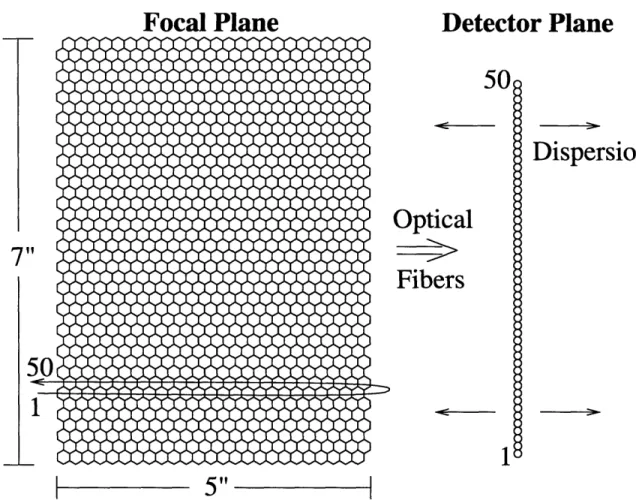
3-1 IFU focal-plane to detector-plane mapping .
3-2 Factorization of IFU spectroscopic flat-field imr 3-3 IMACS-IFU model flatfield cross section . . . 3-4 IMACS-f/4 He-Ne-Ar IFU image subsection
3-5 IFU pixel-to-fiber association diagram ....
3-6 Optimal extraction of IMACS-f/2 IFU data .
3-7 IFU night-sky background subtraction ....
3-8 Narrowband spectral component modeling . .
3-9 SDSSJ0037 IFU spectra ...
3-10 SDSSJ0037 IFU imaging ...3-11 SDSSJ2238 IFU spectra ...
3-12 SDSSJ2238 IFU imaging ...3-13 SDSSJ2321 IFU spectra ...
3-14 SDSSJ2321 IFU imaging ...3-15 SDSSJ2302 IFU spectra ...
3-16 SDSSJ2302 IFU imaging ...3-17 SDSSJ0044 iso-wavelength emission-line image
3-18 SDSSJ0044 IFU spectra ...
3-19 SDSSJ0044 IFU imaging ...3-20 SDSSJ0737 IFU spectra ...
3-21 SDSSJ0737 IFU imaging ...3-22 SDSSJ1402 IFU spectra ...
3-23 SDSSJ1402 IFU imaging ...3-24 SDSSJ1630 IFU spectra ...
3-25 SDSSJ1630 IFU imaging ... ag . . . .,.,. . ·. o·,., .,.,.·. ·. ,..o .·.o.,. . . . .. sequence ·. . . . o ·. . . . o.o· .. .,. . . .o. .o. . .oooo .. o.,.3-26 Lensing velocity dispersion versus stellar velocity dispersi 3-27 Power-law mass model constraints from IFU lensing ai
dispersion measurements ... . . . . . . . .. . . . . . . . . . . . .. . .. . . . . . . .. . . . . . . .. . . . . . . . .. . . . . . . . . . . . . . . . . . . . . . . . . . . . . . . . . . . . . . . . . . . . . . . . . . . . . . . . . . . . . . . . . .
ion...
and SDSS velocity-. . . .4-1 HST and IFU image comparison for SDSSJ1402+6321 . . .
4-2 Kolmogorov-Smirnov tests of lens-galaxy observables .... 9 22 28 29 32 34 37 39 39 42 44 45 46 50 52 53 54 55 56 57 58 59 60 61 62 63 64 65 66 67 68 71 78 87 91 L
5-1 Effective radius measurements: SDSS versus HST... 5-2 Power-law index versus stellar velocity dispersion ... 5-3 Mass power-law index versus light power-law index ...
5-4 Projected likelihood of power-law index distribution parameters .
5-5 HST-ACS gravitational-lens modeling of SDSSJ0912+0029 . . .
B-1 SDSS LRG spectra with background-i B-1 (continued) ... (continued) (continued) (continued) (continued) (continued) (continued) (continued) (continued) More SDSS (continued) ·. . . . . . · . . . . · . . . . . . . . · . . . . · . . . . · . . . . · . . . . lens-candidate . . . . . . . . . . . . . . . . . . . . . . . . . . . . . . . . . . . . . . . . . . . .
spectra
. . . . galaxy emission . . . .... 112 . . . 113 . . . 114 . . . 115 . . . 116 . . . 117 . . . 118 . . . 119 ... . . .. . .. . . .. . . . .. . 120 ... . . .. . . . .. . . . ... 121 ... .. .. . .. . . .. . .. .. . .. 122 ... .. . . . .. . . .. . .. . . .. . 123 SDSS color (continued) (continued) (continued) (continued) images of . . . . . I .. .. I.. .. . I.. .. . lenses . . . . . . . . . . and lens . .. . .. . .. .candidates .
. . . . . . . . .. . . . . . . . . .D-1 SDSSJ0216-0813 IFU spectrum and narrowband imaging
D-2 SDSSJ0805+3037 IFU spectrum and narrowband imaging
D-3 SDSSJ0928+4400 IFU spectrum and narrowband imaging D-4 SDSSJ0956+5100 IFU spectrum and narrowband imaging
D-5 SDSSJ1029+6115 IFU spectrum and narrowband imaging
D-6 IFU rotation-curve image sequence of SDSSJ1029+6115 D-7 SDSSJ1128+5835 IFU spectrum and narrowband imaging D-8 SDSSJ1155+6237 IFU spectrum and narrowband imaging D-9 SDSSJ1259+6134 IFU narrowband imaging ...
D-10 SDSSJ1409+6105 IFU spectrum and narrowband imaging
D-11 SDSSJ1416+5136 IFU spectrum and narrowband imaging
D-12 SDSSJ1521+5805 IFU spectrum and narrowband imaging D-13 SDSSJ1547+5719 IFU spectrum and narrowband imaging
D-14 SDSSJ1550+5217 IFU spectrum ...
D-15 SDSSJ1702+3320 IFU spectrum and narrowband imaging
D-16 SDSSJ2251-0926 IFU spectrum and narrowband imaging
E-1 HST-ACS lens images ... E-1 (continued) ...
E-1 (continued) ... E-1 (continued) ... E-2 HST-ACS possible-lens images.
E-3 HST-ACS non-lens/non-detection images.
10 95 97 99 100 103
B-i
B-1 B-1 B-1 B-1 B-1 B-1 B-1 B-2 B-2 C-1 C-1 C-1 C-1 C-1 127 129 131 133 135 139 139 140 140 140 141 141 141 142 142 142 143 143 143 144 144 147 149 151 153 155 157 _ __ __ _ . . . . . . . . . . . . . . . . . . . ....
...
...
...
...
. . . . . . . . . . . . . . . . . . . . . . . . . . . . . . . . . . . . . . . . . . . . . . . . . . . . . . . . . . . . . . . . . . . . . . . . . . . . . . . . . . . . . . . .List of Tables
1.1 Approximate overall properties of lens sample ... 15
1.2 Common optical emission lines in air and vacuum ... 17
3.1 IFU spectrograph configurations used ... 37
3.2 Power-law index distribution parameters from IFU lens sample ... 79
5.1 Comparison of IFU and HST Einstein radii ...
96
5.2 Partition of HST-ACS lens sample into velocity-dispersion bins ... 97
5.3 Maximum-likelihood power-law indices under varying assumptions ... 98
5.4 Power-law index distribution parameters from HST lens sample ... 100
A.1 SDSS lens-candidate photometric and spectroscopic parameters ... 108
A.1 (continued) ... 109
A.1 (continued) ... 110
D.1 Other IFU observations . . . ... 138
12
Chapter 1
Introduction and Motivation
In the currently favored cosmological scenario, the matter content of the universe is dom-inated by a cold and dark component of unknown particle species whose only significant
interaction with the smaller baryonic matter fraction occurs through the gravitational force.
This "cold dark matter" (CDM) picture is most strongly required by observations on the largest scales. The CDM scenario holds that galaxies form within the potential wells of extended dark-matter halos which began their collapse while baryonic matter was still ion-ized. In disk galaxies, this view is supported by direct evidence for dark matter from the
observation of rotational velocities that remain approximately constant out to radii at which
the stellar galactic component makes a diminishing contribution.
Unlike disk galaxies, early-type galaxies (E and SO in the Hubble sequence) are pressure-supported stellar systems which do not generally have directly observable circular-velocity profiles, and as such their density profiles are more difficult to determine. The density structure of early-type galaxies is nevertheless of great interest for numerous reasons. First, their structure constitutes a physical record of their formation and evolution processes. Hi-erarchical CDM galaxy-formation theories hold that early-type galaxies are built through the merging of late-types (Kauffmann, White, and Guiderdoni 1993; Baugh, Cole, and Frenk 1996), which should have predictable consequences for the structure of the merger products. The most stringent test of these theories will require precise observational mea-surements of early-type mass profiles. Second, early-type galaxies exhibit great regularity in their photometric and kinematic properties, as described by the well-known "fundamental plane" (FP) relation between velocity dispersion, effective radius, and surface brightness (Djorgovski and Davis 1987; Dressler et al. 1987). The tilt of the FP relative to the simple expectation based on the virial theorem can be understood in terms of a dependence of the
total mass-to-light ratio upon mass. However, additional constraints on the mass
struc-ture of early-type galaxies are needed in order to distinguish between the various effects of differing stellar populations, differing density profiles (or "structural nonhomology"), and differing dark-matter fractions in giving rise to the FP. Finally, detailed measurement of the structure of high-surface-brightness early-type galaxies will enable quantitative tests of the CDM theory on scales where baryonic and radiative processes have significant effects
upon the structure of the host dark-matter halo (e.g. Blumenthal et al. 1986), altering it
significantly relative to the form expected to result from pure dark-matter collapse (e.g. Navarro et al. 1996; Moore et al. 1998).
On larger scales, conclusive evidence for the dominance of dark matter in early-type galaxy halos comes from observation of X-ray halo temperatures (e.g. Loewenstein and
White 1999) and from statistical signals of weak galaxy-galaxy lensing (e.g. Hoekstra et al. 2004). On smaller scales, observational results are less conclusive. Stellar-dynamical mea-surements of local elliptical galaxies (e.g. Gerhard et al. 2001), the statistics of early-type gravitational-lens galaxies (e.g. Rusin et al. 2003b), and combined lensing and dynamical measurements of the few systems amenable to such study (Koopmans and Treu 2002, 2003; Treu and Koopmans 2002, 2003, 2004, hereafter KT) all argue for the presence of a signifi-cant amount of dark matter even on the scale of the half-light radius, leading to an approx-imately constant circular velocity with increasing radius as in disk galaxies. A conflicting picture is put forward by Romanowsky et al. (2003), who analyzed the dynamics of satellite planetary nebulae of several nearby elliptical galaxies and claim to find little evidence for dark matter. Furthermore, Kochanek (2003) has pointed out an apparent conflict between the expected CDM galaxy halo structure and several well-measured gravitational-lens time
delays under the assumption of Ho0 70 km s- 1 Mpc- 1. Due to this persistent uncertainty
about the mass structure and diversity of early-type galaxies (see also Kochanek 2004b), it is important to exploit any and all available techniques to constrain their properties.
Strong gravitational lensing provides the most direct probe of mass in early-type galax-ies: a measurement of the mass enclosed within the Einstein radius. Unfortunately, strong lenses are a rare phenomenon, and new lenses are generally discovered in small numbers through great luck or great effort. The number of currently known galaxy-scale strong
grav-itational lenses is on the order of one hundred1, but many of these lenses are not suitable
for studying the properties of the lensing galaxy. Some of these lens galaxies are either too faint or too overwhelmed by the light of lensed quasars to be studied in detail. Other systems lack confirmed redshifts for the lens and/or source, seriously limiting their utility as astrophysical tools. Finally, the sample of known lenses as a whole has an extremely heterogeneous discovery history that makes their selection difficult to characterize.
This thesis presents the results of a survey for strong galaxy-galaxy gravitational lenses, which has produced a sample of more than 20 previously unknown early-type strong galaxy-galaxy gravitational lenses. These lenses have all been selected spectroscopically from within the Sloan Digital Sky Survey (SDSS) database, and are confirmed by spatially resolved follow-up observations with ground-based integral-field spectroscopy and/or Hubble Space
Telescope (HST) imaging. The details of the selection and confirmation of these lenses will
be presented in subsequent chapters; the approximate overall properties of the lens sample are given for reference here in Table 1.1.
The new lenses we present here are of great interest for numerous reasons. First, both lens and source redshifts are known from the outset for all of our gravitational lenses. Second, our lenses are all amenable to accurate photometric and stellar-dynamical
mea-surements. Thus the Einstein radii of lenses can be combined with a measurement of the
line-of-sight velocity dispersion profile and the shape of the luminosity density of the lens galaxy to derive powerful constraints on the radial density profile of the lens galaxy through the Jeans equation. Only a handful of previously known strong lenses are amenable to this type of analysis (see KT). In addition, the extended lensed source galaxy images in our systems offer more constraints on the lensing galaxy mass profile than can generally be ob-tained from quasar lenses. Finally, the technique by which we select our lenses is relatively easily characterized, and thus statistical tests of the lens sample should be tractable.
The power of extended lensed images to constrain the gravitational potential of the lens-ing mass was originally considered in the context of radio lenses (e.g. Kochanek et al. 1989;
1see the CASTLES gravitational-lens database at http://cf a-wwv.harvard. edu/castles/
14
Quantity
Median + Standard Deviation
Zlens - 0.21 i 0.08 Zsource ; 0.53 i 0.13 Re 2 ?1 i 0!9 7.5 ± 3.1kpc r-magnitude ; 17.4 ± 0.7aV
-
276
i47 km s
- 1 OE P 1'.'25 ± 0'28 ME - 2.6 i 1.3 x 101 1M®Table 1.1: Approximate overall properties of the sample of new lenses presented in this
thesis. Given are the approximate median and standard-deviation values for various quan-tities. Re is the de Vaucouleurs-model effective radius, a, is the luminosity-weighted stellar velocity dispersion as measured by SDSS, E is the isothermal lens-model Einstein radius, and ME is the lensing mass enclosed by the Einstein radius. With the exception of Zsource and OE, all values given apply to the lens (foreground) galaxy rather than the source
(back-ground) galaxy.
Langston et al. 1990; Kochanek and Narayan 1992), which often show spatially resolved lobes at high resolution, and has also been used to model strong-lensing galaxy clusters with resolved lensed images of background galaxies (e.g. Tyson et al. 1998). Strong galaxy-galaxy lenses such as we present have not previously been known in large enough numbers to constitute a significant class of object, but the promise and formalism of strong galaxy-galaxy lensing has also been developed in the literature. Miralda-Escude and Lehar (1992) have estimated that there should be approximately 100 optical Einstein rings per square degree down to a source-magnitude limit of B = 26. Kochanek et al. (2001) develop a method for using the extended infrared Einstein ring images of lensed-quasar host galaxies to break degeneracies in lens models based only on the quasar-image astrometry. Warren and Dye (2003) describe a method for modeling lenses with extended source images that is non-linear in the lens parameters but linear in the source surface-brightness distribu-tion, which is applied by Dye and Warren (2005) to the lens system 0047-2808 (Warren et al. 1996), perhaps the most well-known strong galaxy-galaxy lens (also spectroscopically discovered).
1.1 Conventions Observed in the Thesis
Here we describe a number of terminological and notational conventions that will be used throughout the thesis, including several "reserved symbols" that will refer always to the same quantities.
Throughout this thesis, we will be concerned with both two-dimensional (projected
onto the plane of the sky) and three-dimensional galactocentric2 radial coordinates. We
will consistently refer to the 2D radial coordinate as R and to the 3D radial coordinate as
r. Note however that depending upon the context, R may be considered in angular units
or in physical units. We will also work extensively with both 2D and 3D power-law density
2
not Galactocentric
models, of the form
i(R)
oc R
-, p(r)
oc r
- .(1.1)
We will consistently refer to the 2D power-law exponent as qr and to the 3D exponent as y. These exponents will also be called "power-law indices" and "logarithmic slopes" somewhat
interchangeably. Note the adopted sign convention, such that positive 77 and y give densities
that decrease with increasing radius, with larger and y giving more steeply falling (or
centrally concentrated) densities. Also note that, as may be verified trivially, a model with
a particular value has = - 1 in projection, though expressing the relationship between
the 2D and 3D normalization factors requires either numerical integration or evaluation of
the hypergeometric function 2F1.
The astronomical systems that are the subject of this thesis show two redshifts along the
same line of sight: we denote the foreground redshift by FG and the background redshift
by ZBG- We will often avoid the common notation ZL and zs (for "lens" and "source"),
since not all systems necessarily exhibit strong lensing. We refer to the luminosity-weighted velocity dispersion of the foreground galaxy as measured by SDSS within a seeing-blurred circular aperture of 3" diameter as o,. The effective (or half-light) radii of de Vaucouleurs models fitted to galaxy imaging data are denoted by Re, and are quoted at the intermediate axis (the geometric mean of the major and minor axes) for elliptical models. The
minor-to-major axis ratio of elliptical mass and light models is denoted by q, with 0 < q < 1 by
definition.
The spectroscopic data in this thesis have all been reduced with respect to a vacuum wavelength baseline and a heliostationary (a.k.a. heliocentric) reference frame. The official
motive behind this choice is that redshifts apply in the strict sense to wavelengths in
vac-uum and not in air, although the nonlinearity of the air-to-vacvac-uum correction is essentially negligible at our spectroscopic resolutions. (The errors incurred by redshifting air rather
than vacuum wavelengths would be < 3kms -l, or 5% of an SDSS pixel.) The practical
motive is that the reduced SDSS spectra that are the starting point for this research are expressed in vacuum wavelengths. In the text we will refer to the atomic transitions of astronomical emission lines by their common air-wavelength names; spectroscopic plot an-notations use vacuum values for consistency with the data. Table 1.2 gives the air and vacuum wavelengths of atomic transitions commonly seen as optical emission lines, related through the air-to-vacuum transformation of Morton (1991).
Throughout this thesis, we assume a cosmological model with QM = 0.3, QA = 0.7, and
Ho = 70h70 kms-1Mpc-l (with h70 = 1).
1.2 Structure and Content of the Thesis
This thesis is organized into chapters corresponding to distinct stages of a survey for new gravitational lenses. The content is the original work of the author (ASB), with much advice from the supervisor (SB). Chapter 2 describes the method used for the systematic spectro-scopic selection of strong gravitational lens candidates, and was published in similar form as Bolton et al. (2004). This project was originally suggested by SB as a survey for lensed Lyman- emitting galaxies within the SDSS luminous red galaxy spectroscopic database; a pilot project was presented by Burles et al. (2000). The idea to re-orient the survey toward more abundant, lower-redshift multi-emission-line lens candidates was conceived by ASB, and all novel methods presented in Chapter 2 were conceived and implemented by ASB.
Chapter 3 presents the results of an observational campaign to confirm and model 16
Line Name Air Wavelength (A) Vacuum Wavelength (A) [O II] 3727 3725.94, 3727.24 3727.00, 3728.30 HA 4101.734 4102.892 Hy 4340.464 4341.684 Hfl 4861.325 4862.683 [O III] 4959 4958.911 4960.295 [O III] 5007 5006.843 5008.239 [N ii] 6548 6548.05 6549.86 Ha 6562.801 6564.614 [N ii] 6583 6583.45 6585.27 [S ii] 6716 6716.44 6718.29 [S II] 6730 6730.82 6732.68
Table 1.2: Common optical emission lines in air and vacuum
strong lenses from the candidate sample using high-resolution integral-field units (IFUs) on the Gemini and Magellan telescopes. The successful proposals to obtain this data were
written and submitted by ASB. The observations were planned and the targets selected
by ASB, in consultation with SB. Most Magellan IFU data were obtained directly by ASB during classical observing runs; GMOS IFU data was obtained through queue-scheduled observations following phase II specification by ASB. The dedicated IDL-based IFU data-reduction software described in Chapter 3 was written almost entirely by ASB, with some code contributions from SB. Much of the IFU software calls upon pre-existing lower-level
routines included in the IDLUTILS and IDLSPEC2D software distributions3. The b-spline
strategy for fitting the night-sky spectrum to the non-rebinned spectral data is implemented
in the SDSS spectroscopic pipeline, and the flatfielding and extraction strategy implemented for the IFU data was suggested by SB. The IFU narrowband imaging and gravitational-lens modeling techniques presented in Chapter 3 were all conceived and implemented by ASB. The idea to consider a spherical de Vaucouleurs model embedded in a power law potential was suggested within the context of collaboration with Leon V. E. Koopmans, Tommaso Treu, Leonidas A. Moustakas, and SB; a similar calculation carried out by LVEK was included in Bolton et al. (2005). The implementation and exposition of this method in Chapter 3, and the inclusion of the mass-normalization considerations of § 3.6.2, are the work of ASB.
Chapter 4 presents observational results from a Hubble Space Telescope (HST) Snapshot Survey targeting spectroscopic gravitational lens candidates identified by ASB. This survey is a collaboration between ASB, SB, LVEK, TT, and LAM. Chapter 4 consists of the
material of the first paper from the survey, currently in preparation. All material in this
chapter is the work of ASB. The b-spline+multipole galaxy fitting technique used to achieve nearly Poisson-limited residual images was suggested by ASB, coded by SB, and applied to the HST-ACS data by ASB.
Chapter 5 makes use of singular isothermal ellipsoid Einstein-radius parameters mea-sured from residual ACS lens images by LVEK. All other analysis in the chapter is by ASB, although as in Chapter 3 the de Vaucouleurs+power law calculation was suggested by collaborators.
3
http://spectro.princeton.edu/idlspec2d_install.html
18
Chapter 2
Spectroscopic Discovery of
Intermediate-Redshift
Star-Forming Galaxies Behind
Foreground Luminous Red
Galaxies
In this chapter we describe our method for selecting spectroscopic gravitational lens candi-dates from within the Sloan Digital Sky Survey database, which produced an initial catalog of 49 lens candidates selected from a sample of 50996 luminous red galaxies and published in Bolton et al. (2004). We identify this sample of potentially lensed star-forming galax-ies through the presence of background oxygen and hydrogen nebular emission lines in the spectra of massive foreground galaxies. This multi-line selection eliminates the ambiguity of single-line identification and provides a very promising sample of candidate galaxy-galaxy lens systems at low to intermediate redshift, with foreground redshifts ranging from 0.16 to 0.49 and background redshifts from 0.25 to 0.81. As well as describing the spectroscopic selection algorithm, we present a noise modeling technique that we use to control the in-cidence of false-positive emission line detections. We present ground-based imaging of two
candidates that show evidence for strong gravitational lensing, and make an approximate
calculation of the number of bona fide strong lenses expected within the candidate sample.
2.1
Introduction
In its strongest form, gravitational lensing produces unmistakably distorted, amplified, and
multiple images of distant astronomical objects. It is therefore not surprising that the
majority of known galaxy-scale gravitational lens systems have been discovered through imaging observations. However, a small number of lenses have been discovered spectro-scopically, with the spectrum of a targeted galaxy showing evidence of emission from a background source and follow-up imaging revealing lensing morphology. The three most se-cure examples are the lensed quasars 2237+0305 (Huchra et al. 1985) and SDSS J0903+5028 (Johnston et al. 2003) and the lensed Lyman-a emitting galaxy 0047-2808 (Warren et al. 1996). Several authors have made predictions for the frequency of lensed quasar discoveries
in galaxy redshift surveys (Kochanek 1992; Mortlock and Webster 2000, 2001). Others, inspired by the discovery of 0047-2808, have undertaken spectroscopic searches for lensed Lyman-a-bright galaxies (Hewett et al. 2000; Willis 2000; Hall et al. 2000; Burles et al. 2000). The idea behind such searches is that a massive foreground galaxy should act as an effective gravitational lens of any object positioned sufficiently far behind it and at small enough impact parameter, and any emission features from such lensed objects should be detectable in the spectra of the foreground galaxy. Therefore a search for discrepant emis-sion features in galaxy spectra can lead to a sample of gravitational lens systems that would not be discovered in broadband imaging searches due to faintness of source relative to lens. This "lenses-looking-for-sources" approach is complementary to lens searches such as the recently completed Cosmic Lens All-Sky Survey (CLASS; Myers et al. 2003; Browne et al. 2003) which proceed by targeting sources and looking for evidence of an intervening lens. In addition to the optical Einstein ring 0047-2808 mentioned above, Hewett et al. (2000) have published one more spectroscopic galaxy-lens candidate. In contrast to the spectro-scopic discovery method, Hubble Space Telescope (HST) imaging has had some success in detecting strong galaxy-galaxy lenses, as described by Crampton et al. (2002), Ratnatunga et al. (1999), and Fassnacht et al. (2004); spectroscopic confirmation remains a challenge in most cases.
With its massive scale and quality of data, the spectroscopic component of the Sloan
Digital Sky Survey (SDSS) provides an unprecedented opportunity for spectroscopic galaxy-galaxy gravitational lens discovery. Here we describe the first results of such a search within a sample of -51,000 SDSS luminous red galaxy (LRG) spectra (Eisenstein et al. 2001 hereafter E01): a catalog of candidate lensed star-forming galaxies at intermediate redshift. The lens candidates we present were detected by the presence of not one but (at least) three emission lines in the LRG spectra identified as nebular emission from a single background redshift: [O II] 3727 and two out of the three of H/, [O III] 4959, and [O III] 5007. This
implies a maximum redshift of z 0.8 for any candidate lensed galaxies: at higher redshifts,
[O III] emission moves redward of the SDSS spectroscopic wavelength coverage.
The lensing cross section of a particular foreground galaxy is lower for intermediate-redshift sources than high-intermediate-redshift sources, and in this sense the lens survey we describe
here is at a disadvantage relative to searches for lensed high-redshift Lyman-a emitters. However, the identities of the emission lines in the sample we present here are absolutely unambiguous. This cannot be said for spectroscopic Lyman-a lens candidates, which are typically detected as single discrepant emission lines and are difficult to distinguish from lower-redshift emission or (in the case of a huge survey such as the SDSS) non-astrophysical spectral artifacts. Our spectroscopic lens survey based on multiple-line detection has further advantages. First, the source redshift of any lensed galaxies will be known from the outset, along with the redshift of the lens galaxy. This is a tremendous advantage because knowl-edge of both redshifts in a strong lens system is needed to establish the cosmic geometry and fix the absolute mass scale of the lensing constraints, but obtaining both of these redshifts is typically a major observational hurdle. Second, for a given limiting line flux, star-forming
galaxies at intermediate redshift are more numerous on the sky than Lyman-a emitters
at high redshift (see Hippelein et al. 2003; Maier et al. 2003), and hence strong lensing events could be more frequent despite decreased lensing cross sections. Correspondingly, the non-lensed source population should be more amenable to study and characterization (Hogg et al. 1998; Drozdovsky et al. 2005 for example), facilitating lens statistical analysis. Finally, intermediate-redshift lensed galaxies will probe the mass distribution of the lens population in a systematically different manner than do high-redshift sources.
2.2 Search Sample
The Sloan Digital Sky Survey is a project to image roughly one-quarter of the sky in five
optical bands and obtain spectroscopic follow-up observations of 106 galaxies and 105
quasars. York et al. (2000) provide a technical summary of the survey, Gunn et al. (1998) describe the SDSS camera, Fukugita et al. (1996), Hogg et al. (2001), and Smith et al. (2002) discuss the photometric system and calibration, Pier et al. (2003) discuss SDSS astrometry, Blanton et al. (2003) present the spectroscopic plate tiling algorithm, and Stoughton et al.
(2002) and Abazajian et al. (2003) describe the survey data products. Approximately
12% of the galaxy spectroscopic fibers are allocated to the LRG sample (E01), selected to consist of very luminous ( 3L,), and hence massive, early-type galaxies at higher redshift than the galaxies of the MAIN sample (Strauss et al. 2002). We expect these LRGs to be particularly effective gravitational lenses of any objects positioned suitably behind them, and we concentrate our initial spectroscopic lens survey on them. We also note that LRGs should have little dust, and therefore any lensed background galaxies should suffer minimal extinction. The initial sample for our study consists of 50996 spectra taken between 5 March
2000 and 27 May 2003 of SDSS imaging objects flagged as GALAXY-RED by the photometric
pipeline (Lupton et al. 2001) for passing the LRG "cut 1" described by E01, reduced by the SDSS spectroscopic pipeline (J. Frieman et al., in preparation), and selected to have redshifts between 0.15 and 0.65 as determined by the specBS redshift-finding software (D. J. Schlegel et al., in preparation). The low-redshift cutoff is needed because less massive
galaxies start to pass the photometric cuts below z < 0.15 and pollute the volume-limited
LRG sample; see the discussion in E01 and the bimodal LRG sample redshift histogram in Stoughton et al. (2002 Fig. 14). Later in this thesis we will also present follow-up observations of lens candidates selected by similar techniques from within the SDSS MAIN sample.
In addition to being much more massive than the average galaxy, LRGs have another property that makes them well suited to a spectroscopic lens survey: their spectra are extremely regular and well-characterized (see Eisenstein et al. 2003). To determine the spectroscopic redshift of an SDSS target galaxy with observed specific flux f and one-sigma sky+source noise spectrum ax, the specBS program employs a small set of galaxy eigenspectra (four in the reductions for this study) derived from a rest-frame principal-component analysis (PCA) of 480 galaxy spectra taken on SDSS plate 306, MJD 51690. This eigenbasis is incrementally redshifted, and a model spectrum is generated from the best-fit linear combination to the observed spectrum at each trial redshift, with the final redshift
assignment given by the trial value that yields the overall minimum x2. Although redshift is
the primary output of this procedure, a byproduct of specBS is the best-fit model spectrum itself, f. In the case of LRGs, f typically provides a very detailed and accurate fit to f,
with a reduced X2 of order unity over almost 4000 spectral pixels (roughly 1600 spectral
resolution elements) attained with only 8 free parameters: a redshift, the four eigen-galaxy
coefficients, and the three terms of a quadratic polynomial to fit out spectrophotometric
errors and extinction effects, both of which exist at the few-percent level'. This extremely regular spectral behavior allows us to form residual LRG spectra
f()
_
f - f
(2.1)
'The specBS reductions of public SDSS data are available from the website
http://spectro.princeton.edu.
14
12
r 108
o
-16
a)
4
-4 · ~,,,,n
4000
5000
6000
7000
8000
9000
wavelength (A)
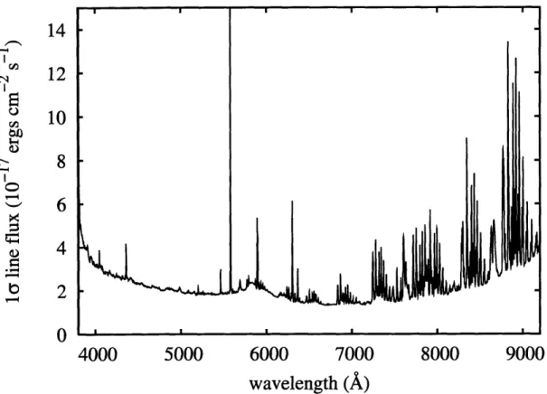
Figure 2-1: LRG sample median line-flux noise spectrum. Shown is the 1-a noise on
best-fit line fluxes for optimally matched Gaussian-shaped residual emission features with spectral width a =1.2-pixel (- 83 km s-l). Reported pixel flux variances have been rescaled as described in § 2.4 prior to the calculation of this noise spectrum.
that are in principle realizations of ar. Nebular emission lines from galaxies along the line of sight other than the target LRG will not be modeled by specBS and should appear as significant features localized in wavelength within these residual spectra. Figure 2-1 shows the median 1-a line flux sensitivity within our LRG residual spectrum sample as a function of wavelength. The (20th, 50th, 80th)-percentile LRG spectra themselves have a median signal-to-noise per pixel of (3.3, 5.1, 9.6) at the SDSS resolution of A/A\A x 1800.
2.3
Candidate Selection
This section describes our candidate selection routine in detail. Briefly stated, we select as
initial candidates those spectra that show both blended [O II] 3727 at SIN > 3 and two out
of the three lines H,/, [O III] 4959, and [O III] 5007 at SIN > 2.5, then cull the candidate
list by applying cuts based on more detailed fits to the presumed emission features, and finally remove any obviously spurious detections. This selection process yields a substantial number of promising systems without an excess of obvious false positives.
2.3.1 Initial Emission Feature Detection
The key element in the first step of our lens candidate selection (described fully in § 2.3.2 below) is a straightforward matched-filtering procedure to search for significant emission
features by fitting a Gaussian line profile at each point in the residual spectrum (Pratt
1978; Hewett et al. 1985). We describe our implementation here so as to be explicit. Let
f(r) be the residual flux in pixel j and oa be the statistical variance of f(r) 2. Also let
{ui}
describe a Gaussian kernel, centered on i = 0, with i running from -ilim to ilim, and normalized such that Ei ui = 1. The maximum-likelihood estimator Aj for the line flux Aj of any {ui}-shaped residual emission feature centered on pixel j is that which minimizesilim
xj=
y Ajui
-
f.t(ji)
/(+i)
(.2)
Differentiating (2.2) with respect to Aj, setting the resulting expression to zero, and solving yields
Aj = c(1) /C(
2)(2.3)
where we have defined the convolutions
C )
f(j+i)ui/(j+i)
(2.4)
(2)-
2/(2.5)
The variance of Aj (under the assumption of uncorrelated Gaussian errors in fr) as
de-scribed by axr) is given by
,j
= 1 /C2)
(2.6)
The signal-to-noise ratio for a fitted Gaussian profile centered on pixel j is therefore
(S/N)j = C)
2)
.(2.7)
Our null hypothesis is an absence of emission features in the residual spectra that should
manifest as the {(S/N)j} being Gaussian-distributed about zero with unit variance: this
should hold at most wavelengths in most spectra. We approach the initial search for emis-sion lines in the residual spectra as a search for significance peaks with (S/N) greater than some threshold value. Although insensitive to goodness-of-fit, this convolution-based de-tection scheme executes quickly ( 15 s per 1000 spectra including file reads on a 2.53GHz Pentium 4 Linux PC) and is therefore well suited to the initial search for residual emission
features within our large spectral sample. We implement the algorithm in the IDL language.
Section 2.4 describes a noise-rescaling process that we employ to control the incidence of false-positive emission-feature detections (due primarily to imperfect sky subtraction)
with-out masking regions of the spectrum.
2.3.2
Multi-Line Background Systems: Detection, Fitting, and Rejection
Multiple emission features at the same redshift will have redshift-independent wavelength
ratios. The fully reduced SDSS spectra have been re-binned at a constant-velocity pixel scale
2
Conversion from units of ergs cm- 2s- 1 A- to units of ergs cm- 2s-1 pixel- 1 is made using the re-binned SDSS spectroscopic pixel scale relation dA = A x 10- 4
ln(10) d(pixels).
of 69 km s-l, giving a redshift-independent pixel offset between features. Our operational scheme is thus to search for coincident (S/N) peaks between multiple copies of a single
filtered residual spectrum that have been shifted relative to one another. For [O II] 3727
detection, we filter each residual spectrum with a a = 2.4-pixel Gaussian kernel (matched to the typical width of blended [O II] 3727 emission seen in SDSS starburst galaxies). We take copies of the same residual spectrum "blueshifted" by integer pixel amounts so as to place H6, Hy, Ho, [O III] 4959, [O III] 5007, [N II] 6548, Ha, [N II] 6583, [S II] 6716, and
[S II] 6730 as close as possible to the geometric-mean wavelength of the [O II] 3727 doublet. These shifted spectra are filtered with a a = 1.2-pixel Gaussian kernel (matched to the typical width of SDSS starburst [O III] 5007 emission), with the sub-pixel part of the line offset relative to [O II] 3727 incorporated by offsetting the kernel. Any pixel in the filtered
SIN spectra with value greater than 3 for [O II] 3727 and value greater than 2.5 for two out of Hp3, [O III] 4959, and [O III] 5007 is tagged as a "hit". A group of adjacent "hit" pixels is reduced to the single pixel with the greatest quadrature-sum SIN for lines detected above the threshold (in effect, the pixel most inconsistent with the null hypothesis). Spectra with more than one isolated hit are rejected. The spectra are only searched in regions that would correspond to emission from > 5000 km s-1 behind the targeted LRG.
The choice to require two significant line detections (rather than just one) in addition
to [O II] 3727 was made in order to control the incidence of false-positive detections. For
Gaussian statistics, the probability of a 3-a or greater positive noise deviation (i.e. SIN > 3)
is P(> 3a+) _ 0.0013; for a 2.5-a positive deviation the probability is P(> 2.5a+) _ 0.0062.
Thus the probability of a 3-a or greater deviation at one wavelength and a 2.5-a or greater deviation at one of three possible other specified wavelengths is
Phit = 3 x P(> 3a+) x P(> 2.5a+) - 2.4 x 10- 5 . (2.8)
For a sample such as ours with 51,000 spectra and - 1000 spectral resolution elements in the searchable redshift range for each spectrum, we would expect on the order of 1000 such noise detections in the sample. Requiring two additional significant detections at the three possible other wavelengths leads to
Phit = 3 x P(> 3a+) x [P(> 2.5a+)]2 _ 1.5 x 10⁻⁷ , (2.9)
and we now expect only on the order of a few to ten false-positive detections within the sample. In principle requiring two additional lines would miss systems with only one addi-tional line even if that line was detected at very high significance. In practice this is not much of a concern since [O III] 4959 and [O III] 5007 always occur with an intensity ratio of 1:3, and a highly significant detection of one will entail a detection of the other as well. The preceding selection leads to 163 single-hit galaxies within our 51,000 spectra. For each hit, we explore a grid of redshift and intrinsic emission-line-width values for the back-ground galaxy to find a best-fit model. At each grid point we fit a Gaussian profile to any emission line initially detected above a 2.0-S/N threshold, with the line center determined
by the trial redshift and width given by the quadrature sum of the trial intrinsic
line-width and the wavelength-dependent spectrograph resolution as measured from arc lines by the SDSS pipeline. [O II] 3727 is fit with a double-Gaussian profile. We adopt as best
values for background redshift ZBG and (Gaussian-a) intrinsic line-width line those that
give the minimum X2 over all detected lines. The ZBG extent of our grid corresponds to +2
pixels, and the explored aline range runs from 0 to 2 pixels (0 to 138 km s-1). 24
Following these fits, we subject the candidate sample to several cuts that are designed to be a quantitative expression of our own judgements about which candidate systems look
real upon spectrum inspection and which do not. First, we reject any system where no
convergent (minimum x2) value for ZBG is found within the explored ±2-pixel range. This
cut tends to reject detections associated with the wings of poorly subtracted night-sky
emission lines. Similarly, we cut systems with no convergent aline between 0 and 2 pixels.
This cut tends to reject systems associated with extended wavelength ranges over which the template model underestimates the galaxy continuum. Next, we compute a total signal-to-noise ratio for the fit, defined as the total best-fit flux in [O 11] 3727 and all other lines initially detected at SIN > 2.5 divided by the quadrature-sum of the 1-a noise from those
line fits, and impose a cut in the total-S/N-x 2 plane (X2 being the X2 per degree of freedom
in the fit). We cut any system with a total SIN less than the greater of 6 and 6 + 3(X2- 1).
This removes both low-SIN candidates and candidates whose X2 values are too high to
be explained by high-S/N emission features showing significant non-Gaussian structure. This cutting procedure reduces the 163 hits to 61 candidate systems. Finally, we prune
12 candidates from the list that survive the automated culling but are clearly explained
by either over-fit LRG stellar absorption, under-modeled LRG line emission, exceptionally poor data quality, or a generally flawed template fit, leaving 49 good candidate systems.
This search for background galaxy emission lines digs rather deep into the noise of our spectroscopic sample. To gauge the incidence of false positives in our final candidate list,
we make a parallel run of the detection, fitting, and automated rejection procedure with the
following rest-wavelength perturbations: H/3 -+ 4833, [O III] 4959 - 4945, and [O III] 5007
-+ 5023. These perturbations alter all of the redshift-independent wavelength ratios among
these lines and between all of them and [O II] 3727; this modified detection procedure no longer selects for real multi-line emission, but only for noise features. The "false candidates"
that result from this perturbed procedure are randomly shuffled along with the candidates
from the original procedure, and all are examined together when making the final pruning judgements. The perturbed procedure yields 88 hits and 7 post-cut candidates; all 7 are
pruned upon inspection without knowledge of their intrinsic falseness. This implies that
the vast majority of our candidates are indeed background galaxies and not simply noise features.
2.4 Noise Modeling
If the model of a purely Gaussian noise spectrum described by ax were correct, then the distribution of scaled residual specific fluxes
xx x (r)/ (2.10)
across all spectra would be Gaussian with unit variance for all wavelengths A. This is unfortunately not the case in our sample. Imperfect night-sky emission-line subtraction and other miscellaneous effects give rise to an excess of high-significance outliers beyond the predictions of a Gaussian model, leading to a deluge of false-positive astronomical emission-line candidates when the procedure described in § 2.3.1 is applied, particularly in
the 7000-9000-A region of the spectrum where the [O III] 5007 line at redshifts z
0.4-0.8 appears. The most drastic solution is simply to mask all sky-afflicted wavelengths.
Rather than concede such vast spectral coverage (which would drastically reduce our survey volume), we describe the observed distribution of scaled residual specific fluxes xv within the
LRG sample with a more detailed empirical noise model. The generally Gaussian behavior of scaled residuals at low significance combined with the excess of high-significance residuals is well described by a mixture of Gaussian and Laplace distributions, expressed parametrically as
p(x) dx = [aexp(-
2/2o
2) + bexp(-lxl/cre)] dx
(2.11)
(For history and applications of the Laplace distribution, see Kotz, Kozubowski, and Podg6rski 2001) The parameters of this distribution are wavelength-dependent, but we suppress this dependence in our notation. The values of a and b are related by normaliza-tion:
r+00
J
p(x) dx = r2
9ga + 2eb =
.
(2.12)
We also fix the following relations between parameters, based on strong correlations observed in free-parameter fits to the distribution at each wavelength:ae = a
9-0.38
,
(2.13)
b = 0.09 x ag(a+b) . (2.14) The result is a one-parameter noise model to fit to the distribution of x\ across the sample at each wavelength. (The numerical values 0.38 and 0.09 are fixed by minimizing the sum
of binned X2 values for fits across all wavelengths.) We relax conditions (2.13) and (2.14)
and fit freely for ae and b at a few isolated locations in the spectrum, where the effects of sky-subtraction residuals are especially strong and the correlations that suggest (2.13) and (2.14) break down-regions near 5577 A, 5894 A, 6305 A, and 6366 A. Additionally, some regions of some spectra are characterized by extreme and correlated excess variance, so for each spectrum we convolve Ix l capped at 5 (to limit the influence of single pixels) with a 100-pixel boxcar filter and exclude from the noise-modeling sample any pixels within a boxcar whose value exceeds 1.25.
We use our fitted noise model to re-scale the reported ua values such that the new
distribution p(x) dx of scaled residual flux values at each wavelength becomes Gaussian, while preserving the position of individual x-values within the cumulative distribution, then proceed as described in § 2.3.1. Both the reported noise ax and the measured residual flux values f(r) contain information about the actual error in the presence of imperfect
subtraction, so it is sensible to base an effective noise rescaling on their ratio x, in this
manner. By fitting the noise distribution parameters independently at each wavelength, we also model the localized effects of individual night-sky lines.
2.5 Candidate Systems
2.5.1
Catalog
Here we discuss our initial catalog of 49 candidate lensed star-forming galaxies selected
to have [O ii] 3727 emission at SIN of 3 or higher and emission from two out of the
three of H/, [O III] 4959, and [O nII] 5007 each at SIN of 2.5 or higher, at a redshift
significantly greater than that of the primary target LRG. Table A.1 lists various properties of the candidate lens systems, together with those of candidates subsequently selected from within the SDSS MAIN spectroscopic sample by similar techniques and targeted for follow-up observation (Chapters 3 and 4). LRG de Vaucouleurs model magnitudes and effective
26
radii are determined from SDSS imaging and photometric reduction. LRG redshifts and
velocity dispersions are as provided by specBS; the software fits for velocity dispersions
ca, using a set of 24 stellar eigenspectra derived from a PCA of the ELODIE spectral
library (Prugniel and Soubiran 2001). These velocity-dispersion measurements have been used successfully to construct the fundamental plane (Bernardi et al. 2003), to measure the velocity function of early-type galaxies (Sheth et al. 2003) and to make a model-based comparison of stellar and dynamical mass estimates of elliptical galaxies (Padmanabhan et al. 2004). We report all av values from the database, although some are likely unreliable;
see the notes of Table A.1. We also report emission-line redshifts of the detected background
galaxies. Using the observed LRG and background redshifts and the observed LRG oa, and assuming a singular isothermal sphere (SIS) LRG luminous+dark matter distribution, we calculate a "best guess" for the angular scale of any lensing that might be present in these
systems as AO = 87r(o2/c2)(DL/Ds). (DLS and Ds are angular-diameter distances from
lens to source and from observer to source.) This is the separation between the two images of a strongly lensed object in the SIS model; it is also the radius of the strong-lensing region of the image plane, and twice the radius of ring images of compact sources directly behind the lens (e.g. Narayan and Bartelmann 1996). For each candidate system we also report
the detected background [O II] 3727 line flux from the best-fit double Gaussian profile. The
reported background line fluxes are simply the fluxes captured by the 3"-diameter SDSS spectroscopic fiber: the shapes and spatial alignments of the background-galaxy images are unknown, and the spectroscopic fibers will in general only record a fraction of their line fluxes. Figure B-1 shows the SDSS discovery spectra and best-fit model spectra, along with close-up views of the residual (data - model) spectra in the wavelength ranges corresponding to redshifted background [O II] 3727, Hp, [O III] 4959, and [O III] 5007.
Although we detect line emission clearly, evidence of background galaxy continuum in
the residual spectra of our candidate systems is scarce. This is not surprising, for three
reasons. One, the LRG sample was selected for particular broadband color and luminosity, and significant background continuum would likely perturb an LRG out of the sample. Two, any faint background continuum present in an LRG spectrum will largely project onto the LRG-redshift eigenspectrum set and low-order polynomial fit used by specBS, and will be subtracted along with the LRG model when forming the residual spectrum. Three, these background galaxies are likely to be high-equivalent-width star-forming systems, and since
their line fluxes are detected just above the noise threshold, the associated continuum will
typically be lost in the noise. Nevertheless, we may obtain a higher signal-to-noise picture of the background galaxies that we detect by constructing a median residual spectrum as follows. First we transform the residual spectra of our candidate systems (i.e. spectra from which template models of the foreground continuum have been subtracted) into units of
erg cm- 2 s- 1 pixel- 1, which is a redshift-independent quantity since the rebinned SDSS
pixels are of constant velocity width. We then shift these residual spectra into the rest
frame of the background galaxy, rounded to the nearest whole pixel, and transform back
to erg cm- 2 s- 1 A-1 . Next we renormalize the spectra by dividing each one by its best-fit
[O II] 3727-flux value. We then take the median value at each pixel, and restore physical
normalization by multiplying this median spectrum by the sample-median best-fit [O II]
3727-flux value. The resulting median spectrum is shown in Figure 2-2. Although there is no discernible continuum in the individual residual spectra, we can see a 4000-A continuum
break in the median spectrum; we also see Hy, Ha, [N II] and [S II] emission lines in addition
to the lines for which we select. This gives further evidence that we have successfully detected and identified real background emission features.
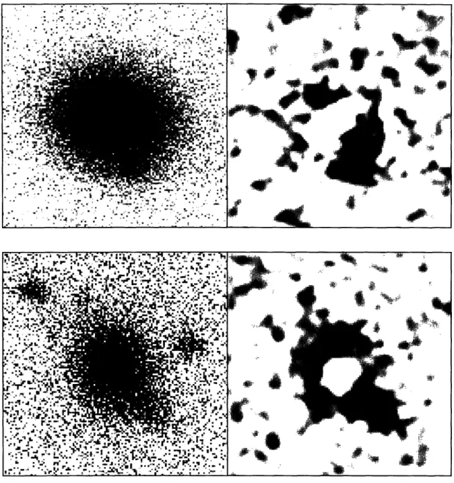
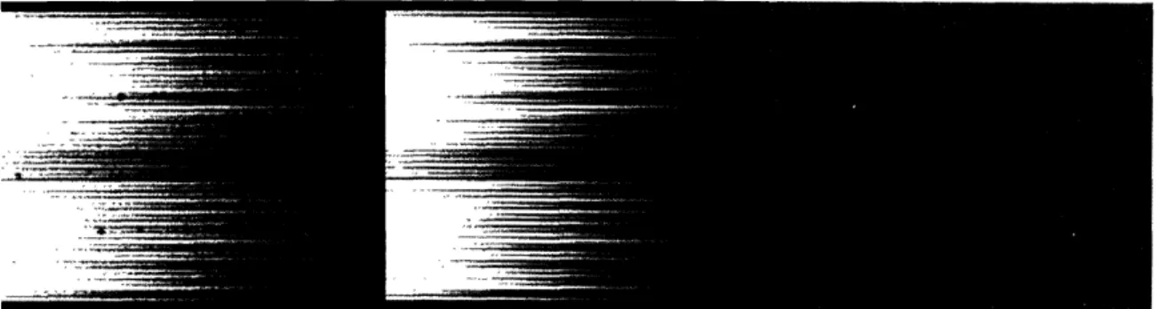
![Figure 3-9: Summed spectra of SDSSJ0037 for fibers with significant background-redshift [O III] 5007 emission-line flux as seen in Fig](https://thumb-eu.123doks.com/thumbv2/123doknet/14461454.520533/52.924.164.759.375.685/figure-summed-spectra-sdssj-significant-background-redshift-emission.webp)
![Figure 3-10: IMACS-2 IFU narrowband imaging of SDSSJ0037 at 8174 A, corresponding to redshifted [O III] 5007](https://thumb-eu.123doks.com/thumbv2/123doknet/14461454.520533/53.924.172.751.190.845/figure-imacs-ifu-narrowband-imaging-sdssj-corresponding-redshifted.webp)
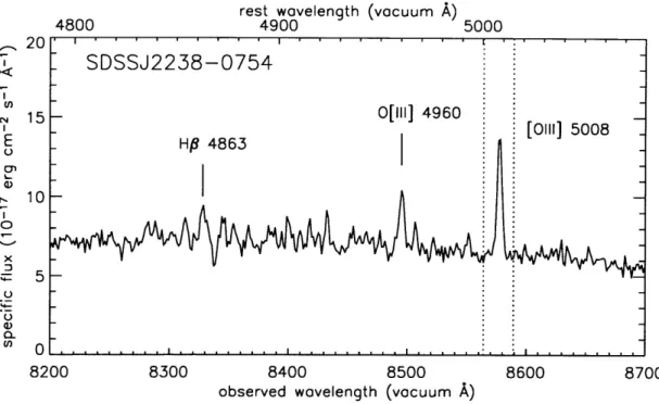
![Figure 3-12: IMACS-2 IFU narrowband imaging of SDSSJ2238 at 8577 A, corresponding to redshifted [O III] 5007](https://thumb-eu.123doks.com/thumbv2/123doknet/14461454.520533/55.924.170.755.188.848/figure-imacs-ifu-narrowband-imaging-sdssj-corresponding-redshifted.webp)
