Supplement of Clim. Past, 16, 743–756, 2020 https://doi.org/10.5194/cp-16-743-2020-supplement © Author(s) 2020. This work is distributed under the Creative Commons Attribution 4.0 License.
Supplement of
Teleconnections and relationship between the El Niño–Southern
Oscilla-tion (ENSO) and the Southern Annular Mode (SAM) in reconstrucOscilla-tions
and models over the past millennium
Christoph Dätwyler et al.
Correspondence to:Christoph Dätwyler (christoph.daetwyler@giub.unibe.ch)
2
S1 ENSO DJF Reconstruction
Figure S1 31-year filtered ENSO index reconstruction. The target ENSO index is shown in red. The
shading indicates its 95% confidence range and the orange shading corresponds to the reference period 1930-1990
3
S2 Proxy Data: Overlaps and climate variable allocation
S2.1 Data overlaps in ENSO and SAM reconstructions
Since both the SAM and ENSO reconstructions share some of the initial proxy record data bases, there are some proxy records contributing to both reconstructions. However, there are only three overlapping proxy records. Hence, this overlap is very small (3 out of 64 in the case of the ENSO reconstructions and 3 out of 34 in case of the SAM reconstruction). The records in question are a coral record (Fiji δ18O, ID 36), a documentary record (from the area de Trujillo, ID85) and an ice core record (Law Dome summer sea salt, ID 441). Our reconstruction methods take out the part of the variability in the proxy records that matches with the target index. Hence we conclude that this minor overlap does not affect the validity of our results when the two reconstructions are compared.
S2.2 Allocation of records to climatic variables for pseudo-proxy generation
As described in the main text, noisy pseudo-proxies from tree and coral archives are generated using proxy system models. To generate the noise-based pseudo-proxies from other archives and the perfect pseudo-proxies, each record is assigned to a climatic variable: coral records are all assigned to temperature. Documentary records are all specific temperature or rainfall proxies and are therefore allocated to the respective variable. Ice core accumulation records are allocated to precipitation, whereas ice core isotope records are allocated to temperature. Tree-ring records usually reflect a mixed signal. Hence, the variable is identified by correlating model temperature and precipitation at the proxy location with the target (ENSO or SAM) index and selecting the variable with the higher correlation. The same procedure was applied to ice core chemical data, where the climate relationship is often not clear. Two records were allocated to a variable based on the literature: Illimani NH4 ice core record: temperature,
Lake Challa warve thickness: precipitation. We note that this process reflects a simplification of the true climate signal, but we argue this is defensible given the number of non-tree and coral records is comparatively small. Also note that the performance of perfect pseudo-proxies is lower than expected in the CESM model because the correlation of local climate to large-scale averages is weaker than in the real-world (Neukom et al., 2018). Fig. 3 shows that the perfect pseudo-proxies do not yield higher reconstruction skill than the real-proxy reconstructions, showing that our correlation-based identification of the “optimal” climate variable for each proxy does not generate pseudo-proxies with unrealistically high proxy-climate relationships in the context of our index reconstructions.
4
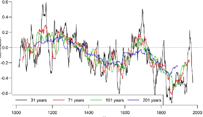
S3 Running correlations between ENSO and SAM for different window
widths and correlations for different window lengths
Figure S2 shows the correlations between ENSO and SAM DJF reconstructions for different window width (31, 71, 101 and 201 years). The correlation over the full time series (using the real-world proxy-based reconstructions) without any filtering (taking lag 1 auto-correlation into account) is -0.07 (not significant). Over 1200-1990 it’s -0.09 (significant, p<0.05), over 1400-1990 it’s -0.16 (significant, p<0.01), over 1600-1990 it’s -0.17 (significant, p<0.01) and over 1800-1990 it’s -0.25 (significant, p<0.01). I.e., we get significant negative correlations as far back as to 1200. There are only few proxy records that contribute to the reconstructions in the early most part which leads to a significant amount of noise. The decrease in correlation strength can also be seen in the pseudo-proxy experiments and also suggests that it is caused by proxy-inherent noise.
Figure S2 Running correlations between ENSO and SAM DJF reconstructions for different window
5
S4 Robustness to choice of different indices for SAM and ENSO
To assess whether a different choice of indices would lead to fundamentally different results, the running correlations between SAM and ENSO reconstructions that are based on different indices are analysed. The running correlations are calculated over a period of relatively good proxy coverage (1800-present) to minimise the chance that the signals are too heavily confounded by proxy noise. For SAM we use reconstructions of the Fogt and Marshall indices and for ENSO reconstructions of the Niño3.4 (based on the two different data sets ERSSTv4 (Huang et al., 2015) and Kaplan (Kaplan et al., 1998)), Niño1+2 and SOI (multiplied by -1). In comparison to the index reconstructions used in this manuscript, we see the most pronounced differences when comparing them to the Niño1+2 index reconstructions. This difference likely arises by the fact that the Niño1+2 index represents a more regional coastal flavour of ENSO. All correlations confirm the significant negative correlations between the two modes of climate variability, except for one case that was not significant (SAM Fogt vs. Niño1+2). All other cases even yield a stronger significant negative correlation (from -0.28 to -0.47, opposed to -0.25 for the index reconstructions used in this manuscript). Hence, we are confident to say that the observed negative correlations do not arise from an artefact of a specific index or choice thereof.
In fact, the comparison of the correlations based on the different indices suggests that the apparent decline of the correlations between ca. 1950-1980 seen in our data (Fig. 1), may be an artefact of the choice of the index (SAM Fogt). Results based on the SAM Marshall suggest that correlations were negative during the entire 20th century, more strongly confirming the general negative correlation pattern seen in the model data.
6
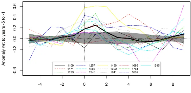
S5 Superposed Epoch Analyses
Figure S4 shows the SEA with 31-year running correlations between ENSO and SAM reconstructions which does not yield a significant response in the years following major volcanic eruptions.
Figure S4 SEA with 31-year running correlations between ENSO and SAM reconstructions. Threshold
for eruptions: 0.15
The SEA with 31-year running correlations between the 13 model ENSO and SAM indices does not yield consistent results. In 8 cases there is no significant response. The results for the 5 cases showing a significant response is as follows:
positive response at year 7
negative response at years 2, 3 and 4
positive response at year 7 and a negative response at year 8
positive response at years 2, 4 and 5 and a negative response at year 8 positive response at year 2
7
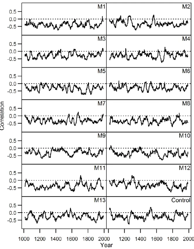
S6 Running correlations between Model ENSO and SAM
Figure S5 Running correlations between ENSO and SAM indices for all 13 CESM model runs
8
S7 Spatial temperature and SLP patterns in the model world during periods
of positive and very strong negative teleconnections using alternative
parameters
Figure S6 Same as Fig. 4 but using a different threshold for positive correlations: two instead of three
standard deviations above the mean, yielding a threshold correlation of +0.07, which is exceeded during 154 years in all available years from 13 transient simulations plus the control run
9
Figure S7 Same as Fig. 5 but using a different threshold for positive correlations: two instead of three
standard deviations above the mean, yielding a threshold correlation of +0.07, which is exceeded during 280 years in all available years from 13 transient simulations plus the control run
10 References
Huang, B., Banzon, V. F., Freeman, E., Lawrimore, J., Liu, W., Peterson, T. C., Smith, T. M., Thorne, P. W., Woodruff, S. D., and Zhang, H.-M.: Extended Reconstructed Sea Surface Temperature (ERSST), Version 4, NOAA National Centers for Environmental Information,
doi:10.7289/V5KD1VVF, 2015.
Kaplan, A., Cane, M. A., Kushnir, Y., Clement, A. C., Blumenthal, M. B., and Rajagopalan, B.: Analyses of global sea surface temperature 1856–1991, J. Geophys. Res., 103, 18567–18589, doi:10.1029/97JC01736, 1998.
Neukom, R., Schurer, A. P., Steiger, N. J., and Hegerl, G. C.: Possible causes of data model discrepancy in the temperature history of the last Millennium, Sci. Rep., 8, 7572, doi:10.1038/s41598-018-25862-2, 2018.