Extension of NPDE for evaluation of nonlinear mixed effect models in presence of data below the quantification limit with applications to HIV dynamic model.

HAL Id: inserm-00740912

https://www.hal.inserm.fr/inserm-00740912

Submitted on 11 Oct 2012

HAL is a multi-disciplinary open access

archive for the deposit and dissemination of

sci-entific research documents, whether they are

pub-lished or not. The documents may come from

teaching and research institutions in France or

abroad, or from public or private research centers.

L’archive ouverte pluridisciplinaire HAL, est

destinée au dépôt et à la diffusion de documents

scientifiques de niveau recherche, publiés ou non,

émanant des établissements d’enseignement et de

recherche français ou étrangers, des laboratoires

publics ou privés.

Extension of NPDE for evaluation of nonlinear mixed

effect models in presence of data below the

quantification limit with applications to HIV dynamic

model.

Thi Huyen Tram Nguyen, Emmanuelle Comets, France Mentré

To cite this version:

Thi Huyen Tram Nguyen, Emmanuelle Comets, France Mentré. Extension of NPDE for evaluation of

nonlinear mixed effect models in presence of data below the quantification limit with applications to

HIV dynamic model.. Journal of Pharmacokinetics and Pharmacodynamics, Springer Verlag, 2012,

39 (5), pp.499-518. �10.1007/s10928-012-9264-2�. �inserm-00740912�

(will be inserted by the editor)

Extension of NPDE for evaluation of nonlinear mixed effect

models in presence of data below the quantification limit with

applications to HIV dynamic model

the date of receipt and acceptance should be inserted later

Abstract Data below the quantification limit (BQL data) are a common challenge in data

analyses using nonlinear mixed effect models (NLMEM). In the estimation step, these data can be adequately handled by several reliable methods. However, they are usually omitted or imputed at an arbitrary value in most evaluation graphs and/or methods. This can cause trends to appear in diagnostic graphs, therefore, confuse model selection and evaluation. We extended in this paper two metrics for evaluating NLMEM, prediction discrepancies (pd) and normalised prediction distribution errors (npde), to handle BQL data. For a BQL observation, the pd is randomly sampled in a uniform distribution over the interval from 0 to the probability of being BQL predicted by the model, estimated using Monte Carlo (MC) simulation. To compute npde in presence of BQL observations, we proposed to impute BQL values in both validation dataset and MC samples using their computed pd and the inverse of the distribution function. The imputed dataset and MC samples contain original data and imputed values for BQL data. These data are then decorrelated using the mean and variance - covariance matrix to compute npde. We applied these metrics on a model built to describe viral load obtained from 35 patients in the COPHAR 3 - ANRS 134 clinical trial testing a continued antiretroviral therapy. We also conducted a simulation study inspired from the real model. The proposed metrics show better behaviours than naive approaches that discard BQL data in evaluation, especially when large amounts of BQL data are present.

Keywords model evaluation · nonlinear mixed effect models · prediction discrepancies ·

normalised prediction distribution errors · limit of quantification · HIV dynamic model

Introduction

Nonlinear mixed effect models (NLMEM), also referred to as population analysis, have gained broad acceptance in longitudinal data analysis since their first applications to pharmacokinetic data, introduced by Sheiner et al in the late 1970s [1, 2]. NLMEM can help us to understand many complex nonlinear biological processes as well as the mechanisms of drug action, the differ-ent sources of variation, e.g., the interindividual variability. NLMEM are also useful to study the progression of chronic diseases under treatment such as chronic infections with hepatitis virus or HIV [3–6]. In HIV infection, the viral load is a widespread marker for the disease progression and decrease of HIV viral load is used to evaluate the efficacy of antiretroviral treatment [4, 7–9]. NLMEM are well adapted to study repeated viral load measurements and different sources of T.H.T. Nguyen · E. Comets · F. Mentré

INSERM, UMR 738, F-75018 Paris, France

Univ Paris Diderot, Sorbonne Paris Cité, UMR 738, F-75018 Paris, France F. Mentré

AP-HP, Hosp Bichat, Service de Biostatistique, F-75018 Paris, France

Corresponding author: T.H.T. Nguyen E-mail:thi-huyen.nguyen@inserm.fr

variation. HIV viral load evolution can be characterised by a complex system of several differen-tial equations [7–11] but in practice, the biphasic decline of HIV viral load under treatment can be simply described by a bi-exponential model. This model is an approximate analytical solution for the complex differential equations system obtained through additional assumptions: a con-stant concentration of CD4+ cells during treatment and no pharmacokinetic/pharmacodynamic (PK/PD) delay [7, 8].

NLMEM are associated with a number of assumptions with regards to the complex nonlinear model structure, variability distributions etc. It is therefore a crucial part of modeling to assess the validity of these assumptions by evaluating how well the model predicts a validation dataset. The validation dataset can be the original dataset that was used to build the model (internal evaluation) or can be another dataset (external evaluation). We define the null hypothesis, H0,

the fact that the tested model describes adequately the validation dataset. Many evaluation methods have been developed and used for assessing NLMEM. The methods based on residuals and prediction errors are the most classical diagnostic tools. However, in the context of NLMEM, these metrics show poor statistical properties, due to the linearization step required in their computation [12]. Another family of evaluation tools, Posterior Predictive Check (PPC), was proposed by Bayesian statisticians [13, 14]. These PPC metrics are also known under the name "simulation-based metrics" as simulations are required in their computation. These methods con-sist in comparing a statistic calculated from the validation dataset with the predictive distribution of the chosen statistic under the tested model. They are shown to present better behaviours than residuals-based methods. Several metrics belonging to this family are now widely used for eval-uating NLMEM, e.g. the Visual Predictive Check (VPC) [15], the Numerical Predictive Check (NPC), the prediction discrepancies (pd) [12] or the normalised prediction distribution errors (npde) [16, 17]. In this family, the prediction discrepancy (pd), an evaluation metric proposed by Mentré and Escolano, is widely used to evaluate NLMEM in PK/PD modeling [12, 18]. In case of repeated measurements, if modelers want to perform statistical tests, npde, a decorrelated version of the metric, should be used instead of pd because pd are correlated within individuals [16–19]. These metrics are now routinely output in NONMEM and MONOLIX, the two most popular software for PK/PD modelling. A library for R (npde) is also available [17].

Data below the limit of quantification (LOQ) is a common challenge in data analysis using NLMEM. In fact,the decline of viral loads below the detection limit is a marker of the efficiency of HIV treatments. Consequently, the proportion of BQL data observed during HIV clinical studies increases with the appearance of more efficient treatments. This is a concern for parameter estimation, since it was shown that common naive approaches such as discarding all these BQL data or imputing them at an arbitrary value (LOQ or LOQ/2) could lead to biased and inaccurate estimates if the percentage of BQL data is high [20–23]. More sophisticated approaches that account for BQL data in the likelihood function were also developed and evaluated such as the M3, M4 methods [22–25], the MCEM algorithm [26] or the extended SAEM algorithm [6]. These methods were shown to allow more accurate and less biased estimates than the naive approaches [6, 22, 23, 25]. However, although BQL data are correctly handled during the estimation step, they are often omitted or imputed at an arbitrary value in most of the current evaluation methods. In this paper, we show how trends can appear in diagnostic graphs when BQL data are omitted from the plots and we extend two evaluation metrics (pd and npde) to take into account these data. As the bi-exponential HIV dynamic model has been used as illustrated example in another study on BQL data [6], we decided to use that model to illustrate the use of the new metrics and to evaluate their properties. We first applied the new metrics to evaluate a HIV dynamic model describing the HIV viral load evolution under a new anti-retroviral treatment. The HIV viral load data were obtained in the COPHAR 3 - ANRS 134 trial, a phase II clinical trial supported by the French Agency for AIDS Research [27]. A simulation study was also carried out to evaluate the graphical use of the two new metrics using diagnostic tools as well as their statistical properties (type I error and power) using statistical tests.

Statistical methods Notations

Let i denote the ith _{individual (i = 1, . . . , N ) and j the j}th _{measurement of an individual}

(j = 1, . . . , ni,where niis the number of observations for individual i). The statistical model for

the observation yijin individual i at time tij is given by:

yij= f (tij, θi) + εij (1)

where the function f is a (nonlinear) structural model supposed to be identical for all individuals, θi is the vector of the individual parameters and εij is the residual error, which is assumed to

be normal with zero mean. We assume that the variance of the error follows a combined error model:

V ar(εij) = (σinter+ σslope× f (tij, θi))2 (2)

where σinter and σslope are two parameters characterizing the error model. We can also assume

a constant error model in which σslope= 0 or a proportional error model where σinter= 0.

The individual parameters θican be decomposed into fixed effects µ representing mean effects

of the population and random effects ηi specific for each individual. We assume frequently an

additive effect, e.g., for the qth_{component of the vector θ} i:

θiq = µq+ ηiq (3)

or an exponential effect:

θiq= µq× exp(ηiq) (4)

It is assumed that ηi∼ N (0, Ω) with Ω defined as the variance - covariance matrix so that each

diagonal element ω2

q represents the variance of the qthcomponent of the random effect vector ηi.

We define Ψ the vector of population parameters, including the vector of fixed effect param-eters µ, paramparam-eters characterizing the distribution of random effect (unknown elements of the variance - covariance matrix Ω) and parameters for residual errors (σslope, σinter), Ψ ={µ, Ω,

σslope, σinter}.

Prediction discrepancies

The null hypothesis assumes that the validation dataset can be described by the model being tested. First, to compute the prediction discrepancy, let pi(y|Ψ ) be the whole marginal predictive

distribution of observations for the individual i predicted by the tested model, it is defined as: pi(y|Ψ ) =

ˆ

p(y|θi, Ψ)p(θi|Ψ )dθi (5)

Let Fijdenote the cumulative distribution function of the predictive distribution pi(y|Ψ ). The

prediction discrepancy is defined as the percentile of an observation in the predictive distribution pi(y|Ψ ), as given by:

pdij= Fij(yij) =

ˆ yij

pi(y|Ψ )dy =

ˆ yijˆ

p(y|θi, Ψ)p(θi|Ψ )dθidy (6)

The discrepancy can be considered as a new "type" of residuals: unlike the "classical" resid-ual or prediction error which is the difference between the observation and a fitted or predicted value, the prediction discrepancy evaluates the position of the observation in its predictive dis-tribution. In NLMEM, the predictive distribution pi(y|Ψ ) has no analytical expression and can

be approximated by MC simulation. In this method, we simulate K datasets using the design of the validation dataset and the parameters of the tested model. The prediction discrepancy can then be calculated as:

pdij= Fij(yij) = 1 K K P k=1 1_ysim(k) ij <yij (7)

where y_ijsim(k) is the simulated observation at time tij for the ith individual. Note that if yij ≤

ysim_ij (k) for all k = 1 . . . K, then pdij = _2K1 . Similarly, if yij ≥ ysimij (k) for all k = 1 . . . K, then

pdij= 1 − _2K1 .

BQL observations are referred to as left-censored observation, denoted ycens

ij . Using the

pre-dictive distribution, we can evaluate its probability of being under LOQ at time tij for the ith

individual, P r(ycens

ij ≤ LOQ) predicted from the model:

P r(ycens ij ≤ LOQ) = Fij(LOQ) = 1 K K P k=1 1_ysim(k) ij ≤LOQ (8) We propose to compute the pd for a left-censored observation ycens

ij , pdcensij , as a random

sample from a uniform distribution over the interval [0, P r(ycens

ij ≤ LOQ)], assuming that the

model is correct.

By construction, pd are expected to follow a uniform distribution U[0, 1]. pd can also be transformed to a normal distribution using the inverse function of the cumulative distribution function Φ of N (0, 1):

npdij= Φ−1(pdij) (9)

where the npd are the normalised prediction discrepancies.

In case of repeated measurements, npd within an individual are correlated which increases the type I error of the test.

Prediction distribution errors

In order to decorrelate pd, Brendel et al [16] proposed to decorrelate the observations and pre-dictions before computing pd by evaluating the mean E(yi) and the variance - covariance matrix

V ar(yi) over the K simulations under the tested model. The mean is approximated by:

E(yi) ≈ 1 K K X k=1 ysim_i (k) (10)

and the variance - covariance matrix is approximated by: Vi= V ar(yi) ≈ 1 K K X k=1

(y_isim(k)− E(yi))(ysimi (k)− E(yi))′ (11)

Both observed and simulated data are decorrelated as follows: y∗ i = V −1 2 i (yi− E(yi)) (12) y_isim(k)∗= V−12 i (y sim(k) i − E(yi)) (13)

and are then used to compute the decorrelated metric, pde, with the same formula as Eq.8 pdeij= Fij∗(y∗ij) = 1 K K P k=1 1_ysim(k)∗ ij <y∗ij (14) The decorrelated pd are called prediction distribution error (pde). The normalised version of this metric, denoted npde, is more frequently used in model evaluation:

npdeij= Φ−1(pdeij) (15)

In the presence of BQL data, we cannot simply decorrelate the vector of observed data yias

it also contains censored observations. One possible approach is to impute these censored data to a value between 0 and LOQ using the distribution of the observations predicted by the model. However, this distribution is unknown and for this reason, we use the uniform distribution of pd to impute values for BQL data as described as followed. We first impute a pd for the censored

observation by randomly sampling in U(0, pLOQ), then using the inverse function of the predictive

distribution Fij to get the imputed value for the BQL observation:

ycens_ij (new)= F_ij−1(pdcens

ij ) (16)

The new vector of observations ynew

i contains both observed values, for non-censored data, and

imputed values for censored data. As for other simulation-based evaluation methods, simulation must be performed by taking into account all factors influencing the observations, we propose to treat simulated and observed data identically. BQL values in the MC samples are therefore replaced by the same imputation method: we calculate pdsim

ij for each yijsim below LOQ in the

simulated data and these ysim

ij are replaced using the same imputation method applied on the

observed data.

ysim_ij (new)= F_ij−1(pdsim

ij ) if yijsim≤ LOQ (17)

As a result, we obtain, after this imputation step, a new vector of observations ynew

i and new

simulated data ysimnew

i . The complete data are then decorrelated using the same technique as

described above.

Under the null hypothesis, we expect pde to follow the distribution U[0, 1] and npde to follow the distribution N (0, 1). However, one should bear in mind that npde are uncorrelated but not totally independent as observations in NLMEM are not Gaussian [18, 28]. To use statistical tests on npde, we have to assume that the decorrelation step renders the pde independent. This can sometimes cause type I errors to be higher than the nominal level [28]. Also, it should be noted that with the proposed method, left censored observations in the validation datasets are imputed using the model to be evaluated and this could lead to loss of power if the model is wrong.

Alternative approaches for computing pd & npde in presence of BQL data

In the previous sections, we proposed a new method for handling BQL data when computing pd and npde. One can think of other approaches to calculate pd and npde in presence of BQL observations. For instance, we could omit all BQL observations in the validation datasets and also discard all the simulated values in the MC samples corresponding to these BQL data. This approach is named "omit obs" method in the paper. Another possible approach, denoted "omit both" method, consists in discarding BQL values in both the validation dataset and the MC samples. In this method, we remove also BQL values in the simulated data in order to compare observations and simulations under the same conditions. However, removing BQL values in the simulated datasets makes the decorrelation become much more complex and the usual decorre-lation method cannot be applied as the variance - covariance matrix cannot be easily calculated. For this reason, we only evaluate this method on the sparse design, where decorrelation step is not required.

Graphs & Tests

Graphs can be used to evaluate visually the distribution of npde. The npde package for R provides 4 types of graphs: (i) q-qplot of the interested metric versus the expected distribution; (ii) histogram; scatterplots (iii) versus time and (iv) versus predicted values (calculated as the mean E(ysim_ij (k)) over the K simulated value of yij). Under the null hypothesis, no trend is

expected to be present in the last two plots. To facilitate visual interpretation, we added in this paper 95% prediction intervals around some selected percentiles (e.g. the 10th_{, 50}th_{, 90}th

percentiles as in the VPC plot) of the observed npde/pd as proposed in [18]. The prediction intervals of the interested metric can be calculated using K MC datasets or by simulating K samples following the expected distribution, e.g., the standard normal distribution. Prediction band can also be added to the q-qplot of npde (pd) versus theorical quantiles of the expected distribution. As pd are correlated, prediction band for the q-qplot must be calculated from the K simulated MC datasets. If we assume that decorrelation renders npde independent, then the

prediction band for the q-qplot of npde can be calculated from K samples simulated from the N (0, 1) distribution.

We can use a statistical test to evaluate the distribution of npde with respect to the expected distribution N (0, 1). To test if a sample follows the N (0, 1) distribution or not, Brendel et al proposed three tests [16]: (i) Wilcoxon signed rank test, to test if the mean is significantly different from 0; (ii) a Fisher test, to test whether the variance is significantly different from 1; (iii) a Shapiro-Wilk test, to test whether the distribution is significantly different from a normal distribution. The global test combines these 3 tests with a p-value corrected using Bonferroni correction for multiple tests: the value reported in the global test is the minimum of the p-value of three component tests multiplied by 3. We can also use an "omnibus" test such as the Kolmogorov-Smirnov to compare the distribution of npde with N (0, 1). It should be noted that the type I error will increase when testing the npd because of correlation between individuals [12, 19].

Clinical data and HIV dynamic model Data

The data used in this paper were collected from the COPHAR 3 - ANRS 134 clinical trial, a phase II multicentric study supported by the French Agency for AIDS Research [27]. In this study, 35 patients infected with HIV and naive to antiretroviral treatment were included and followed up for a period of 24 weeks. All patients received the same treatment with a once daily dose containing atazanavir (300 mg), ritonavir (100 mg), tenofovir disoproxil (245 mg) and emtricitabine (200 mg) during 24 weeks. Viral load was measured at the first day of treatment and at weeks 4, 8, 12, 16 and 24 (corresponding to days 28, 56, 84, 112, 168) after the initiation of treatment. If the viral load at the week 16 was higher than 200 copies/mL, another measurement was added at the week 20. The HIV RNA assays used in this multicentric study had LOQ of 40 or 50 copies/mL. Only viral load under treatment were kept in the analysis.

Methods

We used the bi-exponential model which was proposed by Ding et al [7, 8] and previously used in other studies to describe the dynamic of the viral load obtained in COPHAR 3 - ANRS 134 trial:

f(tij, θi) = log10(P1ie−λ1itij+ P2ie−λ2itij) (18)

where f is the log10-transformed viral load. This model contains four individual parameters θi:

P1i, P2iare the baseline values of viral load and the λ1i, λ2irepresent the biphasic viral decline

rates. These parameters are positive and assumed to follow a log-normal distribution with the fixed effects µ = (P1, P2, λ1, λ2). We tested different error models in order to choose the most

appropriate one. Model selection was based on the log-likelihood ratio test (for nested models) or the Bayesian information criterion (for non nested models). The parameters of the dynamic model were estimated using the extended SAEM algorithm to take into account BQL data (see more about this algorithm in [6]). An additional variable were used to indicate censoring. Parameters were estimated using the MONOLIX software, version 3.2.

Results

A total of 211 measurements of viral load obtained in 35 patients were used for model building, of which, 102 observations (48.3%) were below the LOQ (40 or 50 copies/mL). The spaghetti plot of viral load data in logarithmic scale versus time is presented in Fig. 1.

We first tested and compared several residual error models on the simplest interindividual variability model where no random effect correlation was present. A constant error model was

finally selected. Secondly, we examined different interindividual variability model with or without correlation terms between random effects and a correlation coefficient between the random effects of the parameters P1, P2was found to be significant (with a gain in BIC = 24.3). The optimal

statistical model is composed of (i) a bi-exponential structural model, (ii) an exponential model for interindividual variability with correlation between the random effects of P1, P2, and (iii)

a constant error model on log10viral load. The parameter estimates for the final model are

presented in Table 1. Parameters were well estimated with the relative standard errors about 30% for fixed effect and smaller than 50% for variability. The relative standard error for the fixed effect of P1 was a little higher than 30% but this can be explained by its large interindividual

variability. We also found a high correlation between the random effects of the two parameters P1and P2(ρ = 0.76).

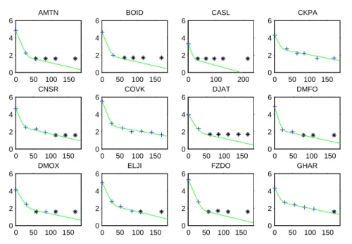
Figure 2 presents some examples for individual fits provided by MONOLIX 3.2. In general, we obtain very good fits for observed data. However, we cannot evaluate how well the model works for BQL data region as in the plots of individual fits, all these data are imputed at the LOQ value.

Some of goodness-of-fit plots provided by MONOLIX of the final model are shown in Fig. 3. The plots of observations versus population predictions and versus individual predictions in-dicate that the model adequately describes data above LOQ. However, clear trends which is a consequence of imputing BQL data at an arbitrary value can be observed in the BQL data region and prevent to evaluate any model misspecification.

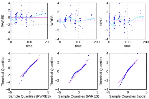
The residual plots are shown in Fig. 4. The residuals (weighted residuals calculated using population predictions WRES, weighted residuals calculated using individual predictions IWRES and npde) seem to distribute homogenously around 0 in the early times when the viral load remains detectable by the HIV RNA assay. However, at later times, where BQL data appear more frequently, we can see important departures of the residuals from 0, that could be explained by the omission of BQL data in residual plots because trends only appear in later times where BQL data are present at high proportions.

The model is also assessed by a visual predictive check (VPC) (Fig.5). Two types of VPC were provided by MONOLIX 3.2 to evaluate the model with respect to both data above and under LOQ. Figure 5(a) is the classical VPC plot, showing the 10th_{, 50}th_{, 90}th _{percentiles for}

observed data over time and their corresponding 90% prediction intervals calculated from K Monte Carlo samples (simulated using the model, the parameter estimates and the design of the building dataset). In the VPC plot, the percentiles of observed data are expected to be within the corresponding prediction bands. This VPC graph shows a good predictive performance of the model for observed data above LOQ. However, as BQL data in the building dataset as well as in K MC samples are imputed at LOQ values, the three observed percentiles and their corresponding prediction bands cannot be correctly calculated. This renders model evaluation in BQL data regions meaningless. Figure 5(b) shows the 90% prediction interval for the observed cummulative proportion of BQL data over time. The fact that this proportion of BQL data remains within the 90% prediction interval supports the choice of final model.

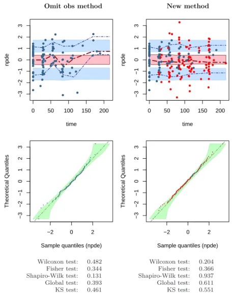
We next illustrated the use of new approach to take into account BQL data when calculating npde on the real data for the final model. Figure 6 shows different graphs, npde versus time and q-qplot of npde versus the distribution N (0, 1), calculated by the "omit obs" or new methods. Once again, we can see that omission of BQL observations in the validation dataset introduces trends in the scatterplot of npde versus time and the model begin to fail in regions where BQL data are frequently observed. Taking into account BQL data by the new approach, trends found in the scatterplot of classical npde disappear in the graph of new npde versus time. Q-qplot and results of different tests performed on the two npde samples show no departure of npde from the normal distribution N (0, 1) in either case; with the original npde however, we could not rule out a loss of power since about half of the observations were omitted (48.3%).

Evaluation by simulation Simulation setting

The model used in the simulation study is inspired from the bi-exponential model built for real data obtained in the COPHAR 3 - ANRS trial. To simulate data under alternative hypotheses (i.e., under false models), we modified the value of the fixed effect and the variability of the parameter λ2, a parameter having direct impact on the percentage of BQL data, of the "true"

model: two false models were obtained by multiplying or dividing λ2 by 2 and two other false

models were generated by multiplying or dividing the variability of λ2(ωλ2) by 3. The parameters used for simulating these models are shown in Table 2.

We chose the main sampling times of the COPHAR 3 - ANRS 134 trial in our simulation study: viral loads were measured on day 0, 28, 56, 84, 112, 168 after the beginning of treatment. In this simulation, we did not simulate the adaptive design which was used in the COPHAR 3 - ANRS 134 trial, where the measurements at week 20 (day 140) depend on the viral load measured at week 16 (day 112). Therefore, we removed the measurement at week 20 in our sampling schedule. We used two designs, both with a total number of 300 observations and with the same number of observations (50 observations) at each time. The first design, called "sparse" design Dsparse, is composed of a total of 300 observations in 300 patients, 1 observation per

individual. This design, which was first proposed and used by Mentré et al in a publication on pd [12], is certainly not realistic but is interesting to study the statistical properties of pd in the absence of within-subject correlations. The second, termed "rich" design Drich, is closer to

the real life data with 50 patients, each of them having 6 sampling times. This design was used to study the impact of within individual correlations on the type I errors of pd and to evaluate the properties of the decorrelated metric, npde. Datasets were simulated under H0with the true

model and under alternative assumptions H1 with the false models described in the previous

paragraph. To study the impact of intra-individual correlation caused by random effects on type I errors, two variability settings S were used: in the first setting, Shigh, the variability of the two

parameters P1, P2are close to those obtained from real data (2.1 and 1.4, respectively); in the

second setting, Slow, the variability for these parameters are both decreased to 0.3. For datasets

simulated with the sparse design, because only one observation is measured for each patient, we cannot study how the two variability settings affect within individual correlation using this design. Therefore, for the sparse design, we chose to use only the high variability setting, which is closer to real life data. Contrarily, for datasets generated with the rich design, both variability settings were used to study the impact of within individual correlation on the new metrics.

In pratical modeling, we can encounter another type of model misspecification: the structural misspecification. For example, data characterising a one-compartment model can be modelled using a two-compartment model. This situation can become true in HIV treatment if a very effective treatment is discovered someday. For this reason, we also want to evaluate the ability of the new method to detect this kind of false model. For this purpose, we chose to simulate a HIV mono-exponential model, Vmono, with the following parameters: P1 = 10000 copies/mL, λ1 =

0.1 day−1_{, ω}

P1 = 2.1, ωλ1 = 0.3 and σinter = 0.14. These parameters are close to those obtained by fitting the real COPHAR 3 data with the mono-exponential model with ωP1, ωλ1 and σinter fixed at the values used for simulating bi-exponential model.

We defined names for different validation datasets, simulated from true model Vt, and from

false models Vf ix1, Vf ix2, Vvar1, Vvar2, Vmono. The last false model, Vmono, is only simulated with the rich design. A set of 1000 validation datasets were then simulated for each scenario. To calculate pd and npde, K = 1000 Monte Carlo samples were simulated with the true model and the design of the underlying validation dataset.

Each simulated dataset was further studied under 3 settings: uncensored, and with two levels of censoring (LOQ = 20 or LOQ = 50 copies/mL), thus generating 3 datasets with different percentages of BQL observations. This allows us to study the behaviour of these new metrics in different conditions. Table 3 shows the proportion of BQL data under the three censoring schemes.

Evaluation of the new npde

To illustrate visually the use of new metric, we first used one randomly selected dataset sim-ulated with the rich design for each scenario under the null hypothesis. The spaghetti plots of these validation datasets are shown in Fig. 7. The figure also shows a randomly selected dataset simulated under each alternative assumption.

We then evaluated the type I errors of chosen statistical tests on the new metric, using 1000 simulated datasets for each scenario. Similarly, under alternative assumptions, we estimated the power of the different tests on new npde using 1000 simulated datasets to detect the corresponding model misspecification. All computations were performed using the statistical software R, version 2.12.2.

Results

Model evaluation under null hypothesis H0

Graphical illustration Scatterplots of npde calculated using the "omit obs" and new methods vs time are shown in Fig. 8 for one dataset simulated under the null hypothesis H0, i.e. with the

true model, for each of the two settings Shigh (high variability, top two lines) and Slow (low

variability, bottom two lines). For each dataset the value of the LOQ used for censoring increases from left (no censoring) to right (LOQ = 20 then 50 copies/mL). This figure clearly shows the necessity of taking these data into consideration in the evaluation step. Indeed, while the model does not show misspecification on the full dataset, trends start appearing in the scatterplots with the "omit obs" npde when a part of the dataset is omitted. These trends disappear with the new npde when BQL data are imputed (red dots).

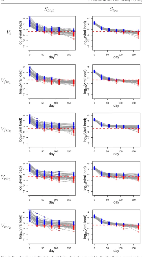
Figure 9 shows the result of the imputation directly on the data, for the same datasets as in Fig. 7. The red dots represent imputed data for observations which were censored, and comparing both figures shows that the imputation step allows to reconstruct a dataset very similar to the original.

Type I error For the sparse design (N = 300, n = 1), npd are identical to npde. For the rich design (N = 50, n = 6), performing tests on npd calculated for rich design results in elevated type I errors: 64.7% (Shighsetting) and 35.0% (Slow setting) compared to 5%. It is not surprising

that the type I error is higher with the Shighsetting as larger values of interindividual variability

used in this setting induce a high correlation within individuals. Table 4 presents the type I error of several statistical tests (Wilcoxon, Fisher, Shapiro-Wilk, global and KS tests) performed for the npde calculated using different methods, under the three designs Dsparse, Drich (Shigh and

Slow). As expected, in the absence of BQL data, the type I errors of different statistical tests for

npde (or npd for sparse design) are close to the significant level (5%). In the presence of BQL data, omitting BQL values (with "omit obs" method) results in a significant increase of type I errors for all designs. The increase in the type I error for the npde obtained with the "omit obs" method under censoring is particularly spectacular under Dsparse, because discarding one BQL

observation means discarding a whole individual. Using the "omit both" method, the type I error is satisfactory. For the new npde, the type I error only increases under Drichin the Shighsetting,

where the interindividual variability is highest. The inflation of the type I errors of the Fisher tests are thought to be the result of the imputation method and the decorrelation step. However, type I errors of the global test remain much lower than those obtained by omitting all BQL data and is very close to the theoretical level.

Model evaluation under alternative assumptions

Graphical illustration The scatterplots of npde versus time, calculated by the new methods, for different false models (Vf ix1, Vf ix2, Vvar1, Vvar2 ), are shown in Fig. 10. In absence of BQL data (first column), under the two alternative hypotheses basing on modifications of fixed effect (Vf ix1, Vf ix2), the scatterplots of npde versus time show a clear trend, which becomes more important

in later times. These trends allow us to detect model misspecification in the second decay phase, which is mainly characterised by parameter λ2 (upper two lines). Under the hypothesis Vvar1, npde are able to detect model deficiencies caused by an increase of the variability of λ2as their

10th _{percentile falls out of its prediction interval. However, npde appear less sensitive to detect}

a decrease of variability, even when there is no BQL data (last line).

These trends in the scatterplots of the new npde versus time remain in presence of BQL data, under the two assumptions Vf ix1, Vf ix2. Nevertheless, as the BQL fraction increases over the time course, the percentiles of npde tend to return to their prediction intervals, especially in regions with a high fraction of BQL data. Thus a high level of BQL data is thought to cause some loss of power. Also, we find in the datasets simulated with Vvar1 that trends can be seen in the Slow setting but not in the Shigh setting; this figure is not shown here as the difference was

only observed under the assumption Vvar1. In fact, it is logic that an increase of variability can be detected more easily on a system of lower interindividual variability. Moreover, the dataset Vvar1 simulated using Slow setting contains less BQL data than those obtained with Shigh (see Table 3). Therefore, model deviation due to modification of variability is more evident with Slow

setting. Finally, on the datasets simulated assuming a decrease of variability of λ2 (Vvar2), the new npde is not able to detect model misspecification, as their observed percentiles are within the corresponding prediction intervals, but this is also the case in the absence of BQL data. Spaghetti plots of imputed data for false models were shown in the last four rows of Fig. 9. As BQL data are imputed using the true model, it is not suprising that the imputed datasets are more comparable to datasets simulated under true model than the corresponding validation datasets. The difference between imputed data and the initial datasets can be more clearly observed in datasets simulated with increased variability.

Figure 11 displays the spaghetti plots of simulated and imputed data as well as the scatterplots of the new npde versus time for the false structure model Vmono. In absence of BQL data, npde

allow us to correctly detect a misspecification of the structural model. When the BQL data fraction increases, the new npde still allow us to identify this kind of misspecification but they seem to be less sensitive. This phenomenon is also observed under other false models. It is also predictable that the spaghetti plots of the imputed data (upper pattern, two last columns) appear to be different to the original simulated dataset as the true model was used to impute BQL data. Power We examined next the powers of statistical tests for the new metrics under several alter-native assumptions (Vf ix1, Vf ix2, Vvar1, Vvar2, Vmono). We also evaluated the power of the "omit both" method under the assumption Vf ix1 as the type I error obtained with this method is also satisfactory. The results are given in Table 5.

In the absence of BQL data, for all the designs, systematic deviations due to changes in fixed effect parameter (Vf ix1, Vf ix2) can be detected by the global test and the KS test with very high powers (100%). The increase in the variability of λ2(Vvar1) can also be detected by KS or global tests on npd or npde with very satisfactory powers when there are no BQL data (100% with the global test and greater than 93% with the KS test). On the contrary, the powers to detect model deficiencies due to a decrease of variability of λ2(Vvar2) are much lower even in absence of BQL observations. The power of the five tests used for detecting a false structure model, Vmono, is very

high, which indicates that npde are a good tool for evaluating this type of model misspecification. In presence of BQL data, using the new method, the powers of the global and KS tests to detect model deviations caused by changes in fixed effect parameter (Vf ix1, Vf ix2) remain very satisfactory (greater than 99%), even when the fraction of BQL data becomes more important. Nevertheless, a very slight loss of power (around 1%) can be observed when LOQ value is raised from 20 to 50 copies/mL. Under the third alternative assumption (Vvar1), the power to detect a modification of variability of λ2in datasets simulated using Shighsetting decreases rapidly when

BQL data fraction increases. The more BQL observations become frequent in the validation datasets, the more important is the loss of power. This can be clearly observed for both Dsparse

and Drich, Shigh. For Drich, Slow, the power to detect the increase of ωλ2remains very satisfactory, even when BQL data are present at very high percentages (100% at LOQ = 20 copies/mL and 99.4% at LOQ = 50 copies/mL). This illustrates that an important change of variability can be more easily detected when interindividual variability is low. Under the assumption Vvar2, the unsatisfactory powers to detect a model deviation could be expected, especially since even when

no BQL data are observed, the power was already very low. Under the alternative assumption based on a false structure model Vmono, the power remains very high even when BQL data are

present at a very high proportion. This high power indicates that the new npde can be used to detect structure model misspecification, a common issue in practical modeling when performing internal evaluation. We notice that in all cases, as the BQL data fraction increases, the power to detect model misspecification decreases, as expected.

Using the "omit both" method, the power for detecting an important change in fixed effect parameter of the false model Vf ix1 in presence of BQL data is much lower than the one obtained with the proposed method for all the test (Table 5). The loss of power when the BQL data proportion increases is also larger in comparison with the new method. Therefore, we did not try to evaluate power of the "omit both" method under other alternative assumptions or under the two rich designs.

Discussion

Evaluation of NLMEM is a crucial issue in population modelling. Therefore, numerous diagnostic tools have been developed and used to examine the adequation of these models. However, most recent evaluation methods are not yet developed to take into account BQL data, even though they are correctly handled in the modelling step by reliable estimation methods. Frequently, in many "goodness-of-fit" graphs, BQL data are discarded or imputed at an arbitrary value such as the LOQ. We have demonstrated in this paper that omitting BQL observations in the validation dataset can introduce patterns or trends in diagnostic graphs when BQL data are present at non-ignorable proportions and thus, could lead to wrong conclusions concerning model adequacy. It is therefore essential to develop new approaches to account for BQL data in the evaluation step.

We focused here on prediction discrepancies (pd) and normalised prediction distribution errors (npde). The two metrics are now widely used to evaluate PK/PD models. Like other diagnostic tools, the recent version of these metrics does not take BQL data into consideration. We proposed in this paper new methods to extend the two metrics to handle BQL data.

We first applied the new methods to evaluate a model obtained from real data. Using the new methods, trends in scatterplots of the classical npde (calculated using the "omit obs" method) disappear from the graph of the new metrics. However, as always in real life, we do not know whether the model is in fact correct for describing the datasets. For this reason, we carried out a simulation study in order to correctly evaluate the properties of the two extended metrics.

The new npde appear to be a promising diagnostic tool in the presence of BQL observations. Indeed, the simulation under H0 shows very satisfactory type I errors that are close to the

significant level for validation datasets with uncorrelated observations. Using the new npde on the datasets simulated with Shigh, we obtain type I errors that are close to 5%, except for some

values that are slightly higher than 5%. Unexpectedly, for about 9% of 1000 datasets, the Fisher test become significant and this value (9%) falls out of the 95% confidence interval of 5%. One possible explanation for the increase of type I errors of the Fisher test is the use of the proposed imputation method. In this method, BQL values if exist in the simulated data (MC samples) are also replaced using the same imputation method applied on the validation data and this step can cause the variance - covariance terms of the observed data to be modified. Indeed, simulated data in each of K MC samples, which correspond to data above LOQ in the validation dataset, may contain some values below LOQ and these BQL values are replaced independently using the imputation method. Thus, when a large number of values in MC samples corresponding to the observed data in the validation dataset are being imputed, the variance - covariance matrix estimated by the imputed MC samples may not reflex correctly the dispersion of the validation data, and change the distribution of the resulting npde. To test that explanation, we used a lower variability setting to study whether within subject correlation could have influence on the variance of npde. For datasets obtained with Slow setting, due to low variability data, MC samples are

much closer to the validation dataset or, in other words, the MC samples are more likely to have a similar number of data above or below LOQ as those of the validation dataset, in comparison with those simulated with Shigh setting, and we obtained lower type I errors of the Fisher test

with Slowsetting. Hence, the increase of type I errors of the Fisher test is probably a result of the

imputation method. However, in our opinion, we should keep treating identically the validation data and simulated data, i.e., applying the same imputation method on both observations and simulations. In fact, in any simulation-based method, we should account for all the factors that can have impact on the generation of the validation dataset during the simulation process. For example, if an adaptive design was used then this step should be reproduced during simulation; otherwise, model evaluation could be misleading [29]. In the proposed approach, we did impute BQL values in the validation dataset using a special method. For this reason, we should reproduce the same process on the simulated data. One possible approach to overcome the limitation of the present imputation method (high type I errors of the Fisher test) is to develop a new imputation method that can take into account correlations with data above LOQ within subject.

It should also be noted that the design used in the COPHAR 3 - ANRS 134 trial is, in fact, an adaptive design as the observations at week 20 are conditionnal on the observations at week 16. However, in this trial, there were only 5 over 35 patients having an additional measurement at week 20 (i.e. 5 samples out of 211 observations). Therefore, we considered that the adaptive design has little impact on the dataset. For this reason, we did not try to reproduce this process during simulation step to compute npde and VPC for the real data. Moreover, the objective of the study is to evaluate a new method for BQL data and hence, we did not simulate adaptive design (as in the COPHAR 3 trial) and assumed that there was no measurement at week 20 in our simulation study.

In spite of some problems of the Fisher tests, type I errors for the npde computed by the new method, especially those of the global test, are very close to 5% and much more lower than those obtained by the "omit obs" method or than those of tests performed on non-decorrelated npd. The type I error of the global test obtained with the "omit both" method is also satisfactory in the presence of BQL data. However, the power of this method to dectect an increased fixed effect is much lower than those obtained with the new method. Contrarily, the power to detect changes in fixed effect parameters of the new npde is very high, even at very high proportion of BQL data. Moreover, we observed an more important loss of power with the "omit both" method when the fraction of BQL data inscreases. The low power of the "omit both" method is the consequence of the loss of available information due to removing BQL data. In the new method, we proposed a method to impute values for BQL data, which means, to add a certain quantity of information into the dataset. This can lead to a gain of power when testing. However, as the information added is based on the use of the model to be validated, a loss of power is expected when BQL data increase. In addition to that, the "omit both" method is likely to have some disadvantages. First of all, a part of simulations which contains BQL values is discarded in the censoring step and only the remaining part of the simulation is used to calculate pd. As a consequence, if a model predicts many BQL values, then we lose an important number of simulations. In this case, pd may not be correctly calculated as the predictive distribution is not well approximated if we do not increase the number of MC samples. Another question is how many simulations we have to increase to assure that pd is correctly calculated. This should not only depend on the number of subjects, of observations but also depends on models and LOQ levels. The second disadvantage is that, when calculating npde for an individual, by removing BQL values in the simulations, we may not obtain vectors of the same length for each time point (each vector corresponds to the simulations at each time point). Thus, the variance - covariance matrix cannot be easily calculated and another method for decorrelating observations/simulations must be investigated. The high power to detect modifications in fixed effects (Vf ix1, Vf ix2) and also misspecifications in structure model (Vmono) of the new npde indicates that the extended metrics are probably good

diagnostic tools for checking the structural model in presence of BQL data. On the contrary, the powers to detect deficiencies of variability model are lower, especially much lower for detecting a decreased variability. This is consistent with the results of previous studies concerning PPC metrics in general, showing that it is difficult to detect a decrease of variability of a parameter [12, 16]. In all cases, we observed a loss of power (more or less important) as the BQL data fraction increases. This behaviour can be anticipated from the proposed methods. Indeed, our method uses the model to compute pd and/or npde: first, to compute the probability to be below LOQ which is used to quantify pd and/or to obtain the predictive distribution for each observation and the inverse of that distribution for imputing BQL observations. This dependency on the model

could account for the loss of power when increasing the proportion of BQL data. In addition to that, the more BQL data are present in the dataset, the less informative data we possess and this affects not only the evaluation step but also the estimation step. Despite this property, the new metrics show better performance than those computed by omitting BQL data in validation data ("omit obs" method) or also in simulations ("omit both" method). Therefore, the new npde is useful in evaluating models with not too high variability parameters and is acceptable to evaluate models with high variability parameters in presence of BQL data.

In the proposed methods, new pd and npde are quantified using a stochastic approach with a single imputation: pd of BQL observation is randomly drawn from a uniform distribution from 0 to the probability for the observation to be under LOQ. Consequently, using the same validation dataset and the same Monte Carlo samples, we could obtain different results (for instance, p-value) when performing the imputation several times. However, in a small simulation study (results not shown), the p-values obtained from different computations were not very different. In fact, we consider the random sampling step to quantify pd as a part of the stochastic properties of simulation-based metrics. For this reason, we performed a unique sampling for each BQL observation and obtained satisfactory type I errors as presented in Table 4. Extension to multiple imputation should be studied.

In this work, we did not include covariates into the model and the simulation study but it would be straightforward to perform another simulation study using this method to evaluate models with one or more covariates. This type of study has been conducted by Brendel et al to evaluate models with covariates on datasets containing no or only few censored data [19].

To test the distribution of npde under the null hypothesis, we used the KS test or the global test that is a combination of three sub-tests: the Wilcoxon test, the Fisher test and the Shapiro-Wilk test. The KS test is a general test that can be used to assess any distribution but it is conservative and may have lower power in comparison with other normality tests such as the Anderson - Darling, Cramer - von - Mises or Shapiro-Wilk tests [12]. In this simulation study, comparing results of the KS test and the global test, we also found that the KS test is less powerful than the global test. It is therefore worth performing the normalisation step to obtain normalised metrics in order to use the global test. In the global test, the Wilcoxon test is used to assess whether the mean of the npde is significantly different from 0 because in real life, we could never know if our npde (npd) follow a normal distributionn. However, the Wilcoxon does not test the mean but the ranks of our npde sample. In consequence, sometimes we observed a significant p-value of the Wilcoxon test while only the value of the variance was changed in the simulation (see Table 5, Vvar1assumption). In fact, for data received in a population-based clinical trial, the sample size is usually large enough to make the normal approximation and we can thus conduct a t-Student test to compare the mean of npde (npd) to 0. If the t-Student test can be used, it might be more powerful than the Wilcoxon test for detecting model deviation due to fixed effect parameters. A perspective of this work is to look for more appropriate tests to test the null hypothesis.

To evaluate a model, a large number of diagnostic tools have been developed, including qualitative (graphs) and quantitative tools (statistical tests). These tests were developed with a purpose to render interpretation more objective. For npde, statistical test results provide us another way interpreting model misspecifications instead of examining several graphs that may be not very easy to be visually investigated (for example, scatter plots of npde vs time or predictions when we have very large numbers of observations at each time). However, the use of statistical tests in model evaluation is still controversial and an agreed-upon solution may not exist. One should bear in mind that statistical tests can fail to reject a poor model due to lack of power or contrarily, a useful model can be refuted by high-power tests. For this reason, it is worth noting that statistical tests should never be used as a sole criterion for evaluating a model as they can be easily misinterpreted or misleading. It is, therefore, very important to understand the limitations of statistical tests and exercise caution in model evaluation.

Because of the complexity of NLMEM, evaluation should necessarily rely on several criteria and methods. As a consequence, it is important to develop new approaches to correctly handle BQL data for other evaluation methods (VPC, NPC, residuals or prediction errors and also individual - based metrics). In the meanwhile, the VPC plot in the presence of BQL data can be presented in several ways. One of the first approaches is to keep original simulations and to

plot the prediction intervals calculated from original simulation while for the observations, the percentiles lower than LOQ are not plotted [23]. Another approach is to impute BQL values in both observations and simulations at the LOQ in order to compute observed percentiles and the corresponding prediction intervals as proposed in MONOLIX 3.2. The final approach is to remove BQL values in both observations and simulations to compute VPC. These methods are usually used when there are BQL data in the validation dataset but they do not account for BQL data. One possible approach to take into account BQL data in the VPC plot is to use the proposed imputation method which is straightforward to be applied to compute metrics where a decorrelation step is not necessary (VPC). Another approach to impute BQL data in VPC plots was recently proposed by Lavielle and Mesa, which consisted in replacing BQL observations of an individual by values simulated with their conditional distribution (calculated using the model and data of that individual) [30]. VPC or residuals such as npde are then computed using these imputed BQL values. This method needs to be evaluated by simulation study.

In conclusion, the new pd and npde are useful diagnostic tools for evaluating NLMEM in presence of BQL data. Although they are not be able to detect model misspecification in some cases (modifications of variability, large fraction of BQL data), they offer better assessment of model adequacy than other classic metrics omitting all BQL data in the validation dataset or also in simulation data. The methods proposed in this paper to take BQL data into account will be implemented in the next version of the library npde for R.

Acknowledgements We would like to thank Professor Cecile Goujard (Hospital Bicêtre), principal inves-tigator of the COPHAR 3 - ANRS 134 trial, to let us have access to the viral load data. We also want to thank Novartis Pharma for funding the PhD of T.H.T. Nguyen during which a part of this work was completed.

References

1. Sheiner LB, Rosenberg B, Melmon KL (1972) Modelling of individual pharmacokinetics for computer-aided drug dosage. Comput Biomed Res 5:441–459.

2. Sheiner LB, Rosenberg B, Marathe VV (1977) Estimation of population characteristics of pharmacokinetic parameters from routine clinical data. J Pharmacokinet Biopharm 5:445– 479.

3. Hughes JP (1999) Mixed effects models with censored data with application to HIV RNA levels. Biometrics 55:625–9.

4. Jacqmin-Gadda H, Thiebaut R, Chene G, Commenges D (2000) Analysis of left-censored longitudinal data with application to viral load in HIV infection. Biostatistics 1:355–68. 5. Perelson AS, Ribeiro RM (2008) Estimating drug efficacy and viral dynamic parameters:

HIV and HCV. Stat Med 27:4647–57.

6. Samson A, Lavielle M, Mentré F (2006) Extension of the SAEM algorithm to left-censored data in nonlinear mixed-effects model: Application to HIV dynamics model. Comput Stat Data An 51:1562–1574.

7. Ding AA, Wu H (1999) Relationships between antiviral treatment effects and biphasic viral decay rates in modeling HIV dynamics. Math Biosci 160:63–82.

8. Ding AA, Wu H (2001) Assessing antiviral potency of anti-HIV therapies in vivo by com-paring viral decay rates in viral dynamic models. Biostatistics 2:13–29.

9. Wu H, Wu L (2002) Identification of significant host factors for HIV dynamics modelled by non-linear mixed-effects models. Stat Med 21:753–771.

10. Perelson AS, Neumann AU, Markowitz M, Leonard JM, Ho DD (1996) HIV-1 dynamics in vivo: virion clearance rate, infected cell life-span, and viral generation time. Science 271:1582–6.

11. Perelson AS, Essunger P, Cao Y, Vesanen M, Hurley A, Saksela K, Markowitz M, Ho DD (1997) Decay characteristics of HIV-1-infected compartments during combination therapy. Nature 387:188–91.

12. Mentré F, Escolano S (2006) Prediction discrepancies for the evaluation of nonlinear mixed-effects models. J Pharmacokinet Pharmacodyn 33:345–67.

13. Gelman A, Carlin JB, Stern HS, Rubin DB (2004) Bayesian Data Analysis Chapman & Hall/CRC, 2nd edn.

14. Yano Y, Beal SL, Sheiner LB (2001) Evaluating pharmacokinetic/pharmacodynamic models using the posterior predictive check. J Pharmacokinet Pharmacodyn 28:171–192.

15. Holford NH (2005) The Visual Predictive Check: superiority to standard diagnostic (Rorschach) plots. PAGE 14 Abstr 738 [www.page-meeting.org/?abstract=738].

16. Brendel K, Comets E, Laffont C, Laveille C, Mentré F (2006) Metrics for external model evaluation with an application to the population pharmacokinetics of gliclazide. Pharm Res 23:2036–49.

17. Comets E, Brendel K, Mentré F (2008) Computing normalised prediction distribution errors to evaluate nonlinear mixed-effect models: the npde add-on package for R. Comput Methods Programs Biomed 90:154–66.

18. Comets E, Brendel K, Mentré F (2010) Model evaluation in nonlinear mixed effect models with applications to pharmacokinetics. J Soc Fr Stat 151:106–128.

19. Brendel K, Comets E, Laffont C, Mentré F (2010) Evaluation of different tests based on observations for external model evaluation of population analyses. J Pharmacokinet Phar-macodyn 37:49–65 Comparative Study Evaluation Studies Journal Article United States. 20. Duval V, Karlsson MO (2002) Impact of omission or replacement of data below the limit

of quantification on parameter estimates in a two-compartment model. Pharm Res 19:1835– 1840.

21. Hing JP, Woolfrey SG, Greenslade D, Wright PMC (2001) Analysis of toxicokinetic data using nonmem: Impact of quantification limit and replacement strategies for censored data. J Pharmacokinet Pharmacodyn 28:465–479.

22. Ahn J, Karlsson M, Dunne A, Ludden T (2008) Likelihood based approaches to handling data below the quantification limit using nonmem vi. J Pharmacokinet Pharmacodyn 35:401–421. 23. Bergstrand M, Karlsson MO (2009) Handling data below the limit of quantification in mixed

effect models. AAPS J 11:371–80.

24. Beal SL (2001) Ways to fit a PK model with some data below the quantification limit. J Pharmacokinet Pharmacodyn 28:481–504.

25. Yang S, Roger J (2010) Evaluations of bayesian and maximum likelihood methods in pk models with below-quantification-limit data. Pharm Stat 9:313–330.

26. Wu L (2004) Exact and approximate inferences for nonlinear mixed-effects models with missing covariates. J Amer Statistical Assoc 99:700–709.

27. Goujard C, Barrail-Tran A, Duval X, Nembot G, Panhard X, Savic R, Descamps D, Vri-jens B, Taburet A, Mentré F (2010) Virological response to atazanavir, ritonavir and tenofovir/emtricitabine: relation to individual pharmacokinetic parameters and adherence measured by medication events monitoring system (MEMS) in naïve HIV-infected pa-tients (ANRS134 trial). International AIDS Society 2010 Abstr WEPE0094 [http://www. iasociety.org/Default.aspx?pageId=11&abstractId=200738161].

28. Laffont C, Concordet D (2011) A new exact test for the evaluation of population pharmacoki-netic and/or pharmacodynamic models using random projections. Pharm Res 28:1948–62. 29. Bergstrand M, Hooker A, Wallin J, Karlsson M (2011) Prediction-corrected visual predictive

checks for diagnosing nonlinear mixed-effects models. AAPS J 13:143–51.

30. Lavielle M, Mesa H (2011) Improved diagnostic plots require improved statistical tools. Implementation in MONOLIX 4.0. PAGE 20 Abstr 2180 [www.page-meeting.org/? abstract=2180].

0 50 100 150 200 2 3 4 5 days lo g10

(

)

Fig. 1 Spaghetti plot of viral load in logarithmic scale versus time from COPHAR 3 - ANRS 134 trial. Data above LOQ are presented as blue circles, data below LOQ are imputed at LOQ in this graph and presented as red circles

0 50 100 150 0 2 4 6 AMTN 0 50 100 150 0 2 4 6 BOID 0 100 200 0 2 4 6 CASL 0 50 100 150 0 2 4 6 CKPA 0 50 100 150 0 2 4 6 CNSR 0 50 100 150 0 2 4 6 COVK 0 50 100 150 0 2 4 6 DJAT 0 50 100 150 0 2 4 6 DMFO 0 50 100 150 0 2 4 6 DMOX 0 50 100 150 0 2 4 6 ELJI 0 50 100 150 0 2 4 6 FZDO 0 50 100 150 0 2 4 6 GHAR

Fig. 2 Some examples of individual fits for the final model. Data above LOQ are presented as blue cross. In this plot, BQL data are imputed at LOQ and are presented as black star symbol

0 1 2 3 4 5 0 1 2 3 4 5 observations predictions Using the population parameters

0 1 2 3 4 5 0 1 2 3 4 5 observations predictions Using the individual parameters

Fig. 3 Observations versus population predicted values and individual predicted values. Observations are plotted as blue closed circles. In these plots, BQL observations are imputed at LOQ values and are presented as black closed circles

0 100 200 −6 −4 −2 0 2 4 PWRES time 0 100 200 −4 −2 0 2 4 IWRES time 0 100 200 −4 −2 0 2 4 NPDE time −5 0 5 −6 −4 −2 0 2 4

Sample Quantiles (PWRES)

Theorical Quantiles −5 0 5 −4 −2 0 2 4

Sample Quantiles (IWRES)

Theorical Quantiles −5 0 5 −4 −2 0 2 4

Sample Quantiles (npde)

Theorical Quantiles

Fig. 4 Residuals (provided by MONOLIX) versus time plots and q-qplots versus the standard normal distribution N (0, 1) of different types of residuals for the final model. In these plots, BQL data are omitted

0 50 100 150 200 1.5 2 2.5 3 3.5 4 4.5 5 5.5 6 days log 10 (viral load)

(a) VPC for observed data

0 50 100 150 200 250 0.0 0.1 0.2 0.3 0.4 0.5 0.6 time BQL data (cum ulativ e frequency)

(b) BQL data fraction over time

Fig. 5 Visual Predictive Check for final model. Figure 5(a) is the classical VPC graph for data above LOQ. BQL data are imputed at LOQ in the graph. The green (dashed and solid) lines represent the 10th_{, 50}th_and

90th_{percentiles for observed data. The shaded blue and pink areas represent 90% prediction intervals for the}

corresponding percentiles calculated from simulated data. Figure 5(b) represents the observed cummulative fraction of BQL data versus time (the fraction of BQL data at a time point is calculated by the ratio between the number of BQL data and the total number of measurements obtained from the beginning to the study to this time) (green solid line) and its 90% prediction interval calculated under the final model (blue shaded area)

0 50 100 150 200 −3 −2 −1 0 1 2 3 time npde 0 50 100 150 200 −3 −2 −1 0 1 2 3 time npde −2 0 2 −3 −2 −1 0 1 2 3

Sample quantiles (npde)

Theoretical Quantiles −2 0 2 −3 −2 −1 0 1 2 3

Sample quantiles (npde)

Theoretical Quantiles

Omit obs method New method

Wilcoxon test: 0.482 Wilcoxon test: 0.204

Fisher test: 0.344 Fisher test: 0.366

Shapiro-Wilk test: 0.131 Shapiro-Wilk test: 0.937

Global test: 0.393 Global test: 0.611

KS test: 0.461 KS test: 0.551

Fig. 6 Scatterplot of npde versus time and the q-qplot of npde for the final model. npde are calculated using the "omit obs" method (left) or the new method (right). npde for data above LOQ are presented by blue closed circles, npde for BQL data are presented by red closed circles. Dashed (blue and dark red) lines in the scatterplot represent 10th_{, 50}th _{and 90}th _{percentiles of the npde corresponding to observed data.}

Light blue and pink shaded areas in the scatterplot are 95% prediction intervals of the selected percentiles calculated from K MC samples. Green shaded area in the q-qplot represents the 95% prediction intervals for the npde sample.

0 50 100 150 −4 −2 0 2 4 6 day lo g10 (vir al load) 0 50 100 150 −4 −2 0 2 4 6 day lo g10 (vir al load) 0 50 100 150 −4 −2 0 2 4 6 day lo g10 (vir al load) 0 50 100 150 −4 −2 0 2 4 6 day lo g10 (vir al load) 0 50 100 150 −4 −2 0 2 4 6 day lo g10 (vir al load) 0 50 100 150 −4 −2 0 2 4 6 day lo g10 (vir al load) 0 50 100 150 −4 −2 0 2 4 6 day lo g10 (vir al load) 0 50 100 150 −4 −2 0 2 4 6 day lo g10 (vir al load) 0 50 100 150 −4 −2 0 2 4 6 day lo g10 (vir al load) 0 50 100 150 −4 −2 0 2 4 6 day lo g10 (vir al load)

V

V

V

V

V

S

S

Fig. 7 Spaghetti plots of different validation datasets simulated using the rich design, under two variability settings Shigh, Slow. Data are not censored and two LOQ levels (20 and 50 copies/mL) are co-plotted as

0 50 100 150 −2 −1 0 1 2 time

Omit obs npde

0 50 100 150 −2 −1 0 1 2 time

Omit obs npde

0 50 100 150 −3 −1 1 2 3 time

Omit obs npde

0 50 100 150 −2 −1 0 1 2 time Ne w npde 0 50 100 150 −2 −1 0 1 2 time Ne w npde 0 50 100 150 −3 −1 1 2 3 time Ne w npde 0 50 100 150 −3 −1 0 1 2 time

Omit obs npde

0 50 100 150 −3 −1 0 1 2 time

Omit obs npde

0 50 100 150 −3 −1 0 1 2 time

Omit obs npde

0 50 100 150 −3 −1 0 1 2 time Ne w npde 0 50 100 150 −3 −1 0 1 2 time Ne w npde 0 50 100 150 −3 −1 0 1 2 time Ne w npde

LOQ = 0 copie/mL LOQ = 20 copies/mL LOQ = 50 copies/mL

S

_high

S

_low

Fig. 8 Scatterplots of npde (calculated using "omit obs" and new methods) versus time for datasets Vt

simulated under the true model. Three levels of censoring were applied on each datasets : 0 copie/mL (first column), 20 copies/mL (second column) and 50 copies/mL (third column).

0 50 100 150 −4 −2 0 2 4 6 day lo g10 (vir al load) 0 50 100 150 −4 −2 0 2 4 6 day lo g10 (vir al load) 0 50 100 150 −4 −2 0 2 4 6 day lo g10 (vir al load) 0 50 100 150 −4 −2 0 2 4 6 day lo g10 (vir al load) 0 50 100 150 −4 −2 0 2 4 6 day lo g10 (vir al load) 0 50 100 150 −4 −2 0 2 4 6 day lo g10 (vir al load) 0 50 100 150 −4 −2 0 2 4 6 day lo g10 (vir al load) 0 50 100 150 −4 −2 0 2 4 6 day lo g10 (vir al load) 0 50 100 150 −4 −2 0 2 4 6 day lo g10 (vir al load) 0 50 100 150 −4 −2 0 2 4 6 day lo g10 (vir al load)

V

V

V

V

V

S

S

Fig. 9 Samples of spaghetti plots of validation datasets presented in the Fig. 7, at a censoring level of 20 copies/mL after the imputation step (see methods).

0 50 100 150 −3 −2 −1 0 1 2 time Ne w npde 0 50 100 150 −3 −1 0 1 2 time Ne w npde 0 50 100 150 −2 −1 0 1 2 3 time Ne w npde 0 50 100 150 −1 0 1 2 3 time Ne w npde 0 50 100 150 −2 0 1 2 3 time Ne w npde 0 50 100 150 −2 0 1 2 3 time Ne w npde 0 50 100 150 −3 −1 1 2 3 time Ne w npde 0 50 100 150 −2 0 1 2 3 time Ne w npde 0 50 100 150 −3 −1 0 1 2 3 time Ne w npde 0 50 100 150 −2 0 1 2 3 time Ne w npde 0 50 100 150 −3 −1 1 2 3 time Ne w npde 0 50 100 150 −2 0 1 2 3 time Ne w npde

LOQ = 0 copie/mL LOQ = 20 copies/mL LOQ = 50 copies/mL

V

V

V

V

Fig. 10 Scatterplots of npde versus time for different validation datasets (Vf ix1, Vf ix2, Vvar1, Vvar2) simulated using the rich design and the high variability setting. npde are calculated by new method that accounts for BQL data. Data above LOQ are presented by blue closed circle, BQL data are presented by red closed circle. Dashed (blue and dark red) lines represent 10th_{, 50}th _{and 90}th _{percentiles of the npde}

corresponding to observed data. Light blue and pink shaded areas are 95% prediction intervals of the selected percentiles corresponding to simulated data