A coupled, two-phase fluid-sediment material model and mixture theory implemented using the material point method

A coupled, two-phase fluid-sediment material model and

mixture theory implemented using the material point

method

by

Aaron S. Baumgarten

Submitted to the Department of Aeronautics and Astronautics

in partial fulfillment of the requirements for the degree of

Master of Science in Aerospace Engineering

at the

MASSACHUSETTS INSTITUTE OF TECHNOLOGY

June 2018

@

Massachusetts Institute of Technology 2018.

Author...

Certified by. .

All rights reserved.

Signature

redacted-A / A

Department of Aeronautics and Astronautics

Signature red acted

May 24, 2018

Ken Kamrin

Associate Professor of Mechanical Engineering

Certified by...

Signature redacted

Accepted by ...

MASSACHUSETTS INSTITUTE OF TECHNOLOGY

JUN 28 2018

LIBRARIES

Thesis Supervisor

Raul Radovitzky

Professor of Aeronautics and Astronautics

Thesis Supervisor

...

Signature redacted...

Hamsa Balakrishnan

Associate Professor of Aeronautics and Astronautics

Chair, Graduate Program Committee

A coupled, two-phase fluid-sediment material model and mixture

theory implemented using the material point method

by

Aaron S. Baumgarten

Submitted to the Department of Aeronautics and Astronautics on May 24, 2018, in partial fulfillment of the

requirements for the degree of Master of Science in Aerospace Engineering

Abstract

A thermodynamically consistent constitutive model for fluid-saturated sediments, spanning dense to dilute regimes is developed from the integral form of the basic balance laws for two-phase mixtures. This model is formulated to capture the (i) viscous inertial rheology of wet grains under steady shear, (ii) the critical state behavior of granular materials under shear, (iii) the viscous thickening of fluid due to the presence of suspended grains, and (iv) the Darcy-like drag interaction for both dense and dilute mixtures. The full constitutive model is combined with the basic equations of motion for each mixture phase and implemented in the material point method (MPM) to accurately model the coupled dynamics of the combined system. Qualitative results show the breadth of problems, which this model can address. Quantitative results demonstrate the accuracy of this model as compared with analytical models and experimental observations.

Thesis Supervisor: Ken Kamrin

Title: Associate Professor of Mechanical Engineering

Thesis Supervisor: Raul Radovitzky

Acknowledgments

The completion of this work would not have been possible without the guidance and support of my research advisor Ken Kamrin and my academic advisor Raul Radovitzky. Raul has continually expected and encouraged me to be a better student and researcher, and Ken has been an invaluable tutor and resource for finding, addressing, and solving challenging problems. To both of these mentors, I am grateful.

I thank my parents and younger brother for their support, encouragement, and the open

invitation for a meal at home if I needed it.

I am thankful for all of my peers in AeroAstro and MechE, especially the AeroAstro

Blackbirds IM hockey team, the members of the Kamrin Group, and my friends in the ACDL, for making this entire experience a positive one. I am also indebted to an innumerable number of friends who have been there for me throughout my time at MIT, the MIT Heavyweight Rowing team, and the 'lab group of destiny'.

In particular, though, I want to thank Alex Feldstein and Connor McMahon, whose patience and friendship I could not do without.

Contents

1 Introduction

2 Theory and Formulation

2.1 Mixture Theory ...

2.1.1 Homogenization of Phases . 2.1.2 Overlapping Continuum Boc

2.1.3 Mass Conservation...

2.1.4 Momentum Balance...

2.1.5 Specific Form of Phase Stres

2.1.6 Specific Form of the Buoyan

2.1.7 Equations of Motion . . . .

ies . . . .

ses . . . t Body F

2.2 Methods for Formulating Drag Law . . . . . 2.2.1 Analytical Method: Stokes's Law 2.2.2 Empirical Method: Darcy's Law . 2.2.3 Simulation Method: van der Hoef's E 2.2.4 Comparison of Methods . . . .

2.3 Material Constitutive Models . . . . 2.3.1 First Law of Thermodynamics . . . .

2.3.2 Second Law of Thermodynamics . . .

2.3.3 Rules for Inter-Phase Heat Transfer . 2.3.4 Helmholtz Free Energy . . . .

2.3.5 Isothermal Assumption . . . .

2.3.6 Strain-Rate Definitions . . . .

2.3.7 Fluid Phase Free Energy Function.

2.3.8 Solid Phase Free Energy Function

2.3.9 Rules for Constitutive Relations . . . 2.3.10 Rules for Drag Law . . . . 2.3.11 Fluid Phase Pore Pressure . . . . 2.3.12 Fluid Phase Shear Stress . . . . 2.3.13 Solid Phase Effective Granular Stress 2.3.14 Solid Phase Plastic Strain-Rate . . . 2.3.15 Solid Phase Stress Evolution . . . . . 2.3.16 Solid Phase Plastic Flow Rules . . .

orce quation 15 17 . . . . 17 . . . . 17 . . . . 20 . . . . 20 . . . . 23 . . . . 24 . . . . 25 . . . . 26 . . . . 27 . . . . 27 . . . . 29 . . . . 31 . . . . 33 . . . . 33 . . . . 34 . . . . 39 . . . . 42 . . . . 42 . . . . 43 . . . . 44 . . . . 45 . . . . 45 . . . . 47 . . . . 48 . . . . 48 . . . . 49 . . . . 50 . . . . 50 . . . . 51 . . . . 52

2.3.17 Proof of Dissipation . . . . 3 Verification of Model

3.1 Com paction . . . .

3.2 Simple Shear Flow . . . .

3.2.1 Fluid Phase Behavior Under Simple Shear Flow

3.2.2 Solid Phase Behavior Under Simple Shear Flow

3.2.3 Combined Behavior Under Simple Shear Flow

3.2.4 Dry Granular Rheology . . . .

3.2.5 Viscous Granular Rheology . . . .

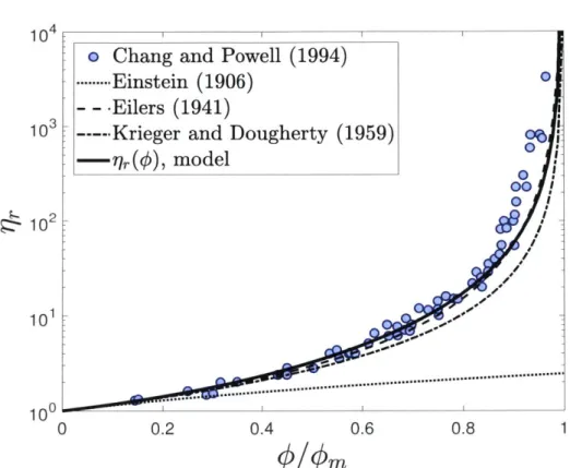
3.2.6 Suspension Effective Viscosity . . . .

4 Numerical Implementation

4.1 Material Point Method Discretization . . . . 4.1.1 Definition of Material Point Tracers . . . . . 4.1.2 Definition of Background Grid Basis . . . .

4.1.3 Definition of Lagrangian Motion . . . . 4.1.4 Weak Form of Momentum Balance Equations 4.1.5 Discrete Mass Balance . . . . 4.1.6 Discrete True Fluid Density Evolution . . .

4.1.7 Discrete Fluid Pore Pressure . . . . 4.1.8 Discrete Fluid Shear Stress . . . . 4.1.9 Discrete Effective Granular Stress Evolution 4.2 Time Marching Procedure . . . . 4.3 Semi-Implicit Effective Stress Algorithm . . . . 4.3.1 Definition of Trial Stress . . . . 4.3.2 Simplification to Scalar Relation . . . . 4.3.3 Complete Algorithm for Stress Update . . .

4.4 Specific Notes About Implementation . . . . 4.4.1 Kinematic Boundary Conditions . . . . 4.4.2 Mixed Boundary Conditions . . . . 4.4.3 Contact Algorithm . . . . 4.4.4 Partial Immersion . . . . 4.4.5 Dynamic Quadrature Error Reduction . . . 5 Results

5.1 Numerical Validation of Model and Method . . . . 5.1.1 Model Fit to Glass Beads . . . .

5.1.2 Granular Column Collapse of Glass Beads

5.1.3 Quasi-2D Flow of Glass Beads . . . .

5.2 Qualitative Results . . . . 5.2.1 2D Circular Intruder . . . . 5.2.2 2D Slope Collapse . . . . . . . . 54 57 57 59 59 60 63 64 64 66 71 . . . . 71 . . . . 74 . . . . 76 . . . . 78 . . . . 79 . . . . ... . . . . 82 . . . . 82 . . . . 83 . . . . 83 . . . . 83 . . . . 84 . . . . 87 . . . . 88 . . . . 89 . . . . 90 . . . . 93 . . . . 93 . . . . 94 . . . . 94 . . . . 94 . . . . 95 97 . . . . 97 . . . . 97 . . . . 98 . . . . 103 . . . . 106 . . . . 110 . . . . 110

List of Figures

2-1 Decomposition of representative mixture volume... 2-2 Definition of overlapping continuum bodies. . . . .

2-3 Inter-phase drag description for dilute mixtures. . . . . . 2-4 Inter-phase drag description for dense mixtures. . . . . .

2-5 _{Determining inter-phase drag for full range of regimes.} 2-6 Comparison between different inter-phase drag laws. . . . 2-7 Physical origin of plastic flow rates. . . . . 3-1 Simple compaction. . . . . 3-2 Simple shearing flow. . . . .

3-3 Comparison of viscous mixture rheology with Boyer et al. 3-4 Effective viscosity of mixture under steady shear. . . . .

Discretization of mixture problem .. . . . . Material point discretization of continuum bodies. . . .

Grid basis functions. . . . . Numerical time integration procedure. . . . . Projection procedure for solid phase plastic flow... Experimental setup from Pailha and Pouliquen [20091. Model fit to results from Pailha and Pouliquen [2009]. Experimental setup from Rondon et al. [20111. . . . . . Column collapse time series. . . . . Pore pressure and shear rate fields. . . . .

Column collapse contours. . . . .

Column collapse pore pressure and runout comparison. Experimental setup from Allen and Kudrolli [2017]. . . Erosion flow time series. . . . .

Erosion flow packing fraction comparison. . . . .

Erosion flow velocity profile comparison. . . . .

Intrusion problem time series. . . . . Slope stability problem time series. . . . .

Effect of water level on slope stability. . . . .

. . . . 74 . . . . 76 . . . . 78 . . . . 88 . . . . 91 . . . . 98 . . . . 99 . . . 100 . . . 102 . . . 102 . . . 104 . . . . 104 . . . . 105 . . . . 107 . . . . 108 . . . . 109 . . . . 110 . . . 111 .. ... 112 [2011]. 18 21 27 29 31 34 53 58 60 67 69 4-1 4-2 4-3 4-4 4-5 5-1 5-2 5-3 5-4 5-5 5-6 5-7 5-8 5-9 5-10 5-11 5-12 5-13 5-14

List of Tables

3.1 Fit Parameters for Figure 3-3 . . . . 66

4.1 Summary of Governing Equations . . . . 72

4.2 _{Summary of Plastic Flow Equations . . . . 73}

5.1 Experimental Setup for Rondon et al. [2011] . . . . 101

5.2 Simulation Parameters for Column Collapses . . . . 103

Chapter 1

Introduction

Mixtures of fluids and sediments play an important role in many industrial and geotechni-cal engineering problems, from transporting large volumes of industrial wastes to building earthen levees and damns. To solve these problems, engineers have traditionally relied on the myriad of empirical models developed in the last century.

These empirical models are derived by coupling relevant experimental observations to an understanding of the underlying physics governing the behavior of these mixtures. The model reported in Einstein [1906] describes the viscous thickening of fluids due to dilute suspensions of grains. The Darcy-like drag law given in Carman 119371 describes the pressure drop in a fluid as it flows through a bed of densely packed grains. The work by Turian and Yuan

[1977]

characterizes the flow of slurries in pipelines. Other models (such as in Pailha and Pouliquen [2009]) describe more complex problems (such as the initiation of submerged granular avalanches); however, each of these models can only provide a description of a specific regime of mixture and flows.

To address an engineering problem which involves complex interactions of fluids and sed-iments spanning many flow regimes requires a more general modeling approach. A natural first step is to model the underlying physics directly by solving the coupled fluid grain inter-actions at the micro-scale (as in the coupled lattice Boltzman and discrete element method, LBM-DEM, proposed in Cook et al. [2004]). Many problems of interest, however, involve far too much material for a direct approach to be computationally viable. We therefore turn to a continuum modeling approach, where the small scale structures and physics are homoge-nized into bulk properties and behaviors. Recent work simulating fluid-sediment mixtures as continua (see Soga et al. [2015]) has shown promise, but the reported results are highly sensitive to the choice of sediment constitutive model (see Ceccato and Simonini [2016] and Fern and Soga [20161); no existing dry granular plasticity models will correctly predict the behavior of saturated soils.

In this work, we begin with the integral form of the basic balance laws for two-phase mixture and carefully formulate a new set of constitutive rules governing the fluid and sed-inent phases of the continuum mixture. Using these rules, we construct a model which recovers the correct limiting empirical behaviors (i.e. dry and viscous granular inertial rhe-ologies, viscous thickening due to suspended grains, Stokes and Carman-Kozeny drags, and

Reynolds dilation) and smoothly transitions between flow regimes covering the range from dense slurry-like flow to dilute suspensions. We discretize the weak form of the governing equations of motion using MPM and validate this implementation against several dynamic experiments involving submerged glass beads. We also consider the application of our model to the problems of slope collapses and intrusion.

Chapter 2

Theory and Formulation

Here we lay out the theoretical framework for the two-phase mixture model. In the formula-tion of this theory, we use the standard notaformula-tion of continuum mechanics from Gurtin et al.

[20101.

In particular, the trace of the tensor A is given by tr A and the transpose by AT. Every tensor admits the unique decomposition into a deviatoric part AO and spherical part

by A = AO + -1 tr(A)1 with 1 the identity tensor.

2.1

Mixture Theory

To develop the model we start by considering a mixture of grains and fluid. We assume that the grains are rough (i.e. true contact can occur between grains), incompressible with density ps, and essentially spherical with diameter d. We also assume that the grains are fully immersed in a barotropic viscofluid with local density pf and viscosity rj. A representative volume of material, , can therefore be decomposed into a solid volume, Q5, and a fluid

volume, Qf, such that Q = Q, U

Qf.

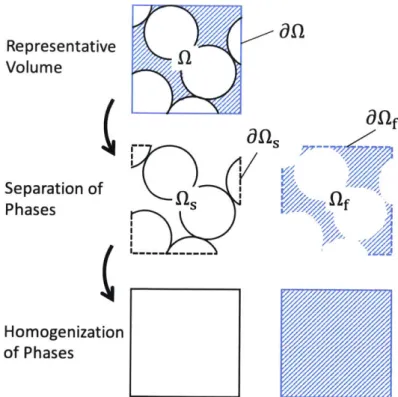
Figure 2-1 shows how this volume is decomposed and the important step of homogenizing the solid volume and fluid volume into two, overlapping continua. In the analysis that follows, b will refer to some field

4

defined on the solid phase, and of will refer to some field

4

defined on the fluid phase. If no subscript is given, then that field is defined on the mixture as a whole.

After defining the effective or homogenized fields, we derive the equations of motion through conservation of mass and momentum. This analysis is essentially identical to that of Bandara and Soga [2015], but explicating it fully here allows us to better present our novel constitutive model and numerical framework.

2.1.1

Homogenization of Phases

The effective densities -p, and pf, and phase velocities v, and vf of the mixture are defined such that conservation of mass and momentum in the continuum correspond to conservation of mass and momentum in the real mixture. For this, we consider a representative volume of

_'- f Representative Volume Separation of Phases s Homogenization of Phases

aflf

ft

Figure 2-1: Pictorial description of the representative volume Q and boundary iQ, the decomposition of the domain into fluid and solid volumes, and the homogenization of the two phases.

material, _{, that contains a large number of individual grains. For the continuum} approxi-mation to be valid, large is defined such that grain-scale phenomena are smoothed out and bulk behavior is captured.

j758 dv = psdv

(2.1)

We now introduce the concept of the local packing fraction and the local porosity. The packing fraction,

#,

_{is defined as the ratio of volume of solid grains to volume of mixture.} The porosity, n, is defined as the ratio of the volume of the fluid to the volume of mixture.

fq dv = fdv f_, dv fu dv jPfdv = pf dv j psvdv = ps vdv

4

pfvfdv = pfvdv

As a consequence of this definition, evaluation of Equation (2.1) over a small represen-tative volume (where small is defined such that changes in the local fields are negligible) leads to three important results. First, the packing fraction and porosity can be calculated from one another (their sum must be one). Second, the effective solid density is equal to the density of the grains scaled by the packing fraction. And third, the effective fluid density is equal to the local fluid density scaled by the porosity.

1- n

Ops (2.2)

pf = npf

We must also define the effective body force acting on each phase in the continuum, bo, and b0o. As with effective density, we require that the integral of the effective body force over

the whole volume be equal to the integral of the actual body force over the phase volume. In the presence of a constant gravity, g, and in the absence of other body forces, we state:

j bosdv = bodv = s gdv

f bodv = body = p gdv

Using the definitions in Equation (2.1), it can be shown that the effective body forces must have the following form,

;5(2.3)

bof =pf g

Lastly, we define the effective Cauchy stress, or, of the mixture according to the integral form of Cauchy's Theorem. This relation is given in Equation (2.4). Since we define the domain boundary dQ such that 8Q =

aQ,

U 9Qf, we can also define the effective Cauchy

stress on each phase, o.). In these expressions, t is the surface traction vector which is a function of the surface normal vector n.

I

o-nda = t(n)da

J

a-,nda = t(n)da (2.4)

j orfnda = t(n)da

It follows from 9Q = 0Q8 U 9Qf, that,

and therefore,

j

crnda=

j

Q nda+ a nda

Since this must hold for any choice of volume Q and boundary &Q, we require,

o as + 0f (2.5)

By defining the effective Cauchy stresses as in Equation (2.4), we show that the total

effective Cauchy stress of the mixture can be decomposed into a stress contribution belonging to the solid phase and another belonging to the fluid phase. This will become important later when we define the constitutive models for the two phases.

2.1.2

Overlapping Continuum Bodies

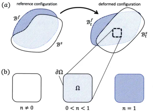
In the previous section, we defined a continuum representation for a mixture of grains and fluid. We now turn our consideration to the continuum mixture model. As shown in Figure 2-2(a), we first define two overlapping continuum bodies. Bs defines the solid phase reference body and Bf defines the fluid phase reference body. At some time t, Bs defines the solid phase deformed body and Bf defines the fluid phase deformed body. These definitions allow us to use the usual continuum definitions of motion, as in Gurtin et al.

[2010.

To determine the behavior of a volume of mixture Q, as shown in figure 2-2(b), we let that volume define a part in each continuum body. The full mixture is defined by the sum of these parts. If the volume of mixture is composed of fluid only, the porosity n is unity. We also enforce that, in the absence of a solid phase, the local solid phase stress is zero, 0, = 0. In this limit, we expect the behavior of the mixture to be identical to that of a barotropic viscous fluid. If the volume of mixture is solid only, the porosity n is not zero (it would only be zero in the limit of vanishing pore space). In this limit, the behavior of the mixture should be identical to that of a dry granular material. To ensure this, we enforce that the local fluid phase stress is zero, of = 0, and that the true fluid density is zero, pf = 0.

2.1.3

Mass Conservation

We now define the equations governing the evolution of the true fluid density (i.e. the density of the fluid that is between the grains), pf, and the effective densities of both phases, p, and Pf. Recalling that the solid grains are assumed incompressible, p, is constant. Since we will often have fields which belong to one phase or another (e.g. p, belongs to the solid phase), it is convenient to define the material derivatives on each phase as follows,

=s aV + _{v,-grad 0}

Dt t _(2.6)

S -

-

+v-gradV

Dt

at

a)

reference configuration deformed configuration

BfB

n*0 0<n<1 n=1

Figure 2-2: (a) Pictorial definition of the reference bodies, BS and Bf, and deformed bodies, Bt' and B{. (b) Parts in the deformed body are always fully saturated with porosity n > 0.

In the limit of a fluid-only volume, the porosity n = _{1. In the limit of a solid-only volume,} we do not let the porosity n go to zero, instead we let the fluid viscosity and bulk modulus go to zero.

enforced by setting the material derivative of solid mass in this volume to zero.

DSjPjdv = 0 Dt in

Using Reynolds' transport relation we can move the material derivative inside of the integral.

J

DPt _{+ 7, div(v,)dv = 0}

This must be true of any choice of volume Q, therefore the strong form statement must also be true. We therefore arrive at Equation (2.7) which governs the evolution of the effective solid density.

S+ P,, div v, = 0 _(2.7)

Dt

We then expand the first term of this evolution law according to Equation (2.6). O + _{v, - grad 7, + ;, div v. = 0}

Expanding with the identity, i, = ops = (1 - n)p,

0(1 - n)ps

+ v. - grad((1 - n)p,) + (1 - n)p, div v. = 0

at

and applying the chain rule,

(I - n) a - Pn + (1 - n)vs grad ps - ps - grad n + (1 - n)p, div vs = 0

at

Pt

Enforcing uniform incompressible grains (ps constant) and dividing out ps, we find,

an

- v - gradn + (1 - n) divv, = 0

at

and therefore, an = (1 - n) divvs - vs - gradn (2.8)

The significance of Equation (2.8) is that we can express the rate of change of the local porosity with knowledge of the current porosity and the solid phase velocity alone. Intuitively this makes sense, the porosity is a measure of the space between grains. We only need a description of the motion of the grains to describe how the porosity is changing.

Turning now to the fluid part defined by the volume Q, we enforce mass conservation in the fluid phase by setting the material derivative of fluid mass to zero.

Df j- dv = 0 Dt L Pf

As before, we use Reynolds' transport relation to move the material derivative inside the integral.

f

Di + pf div vfdv = 0

This must hold for any choice of volume Q, therefore we find Equation (2.9), which governs the evolution of the effective fluid phase density.

Dtf+ pf divvf = 0 (2.9)

We expand the first term according to Equation (2.6),

and replace ;5f above with it's definition in Equation (2.2),

at

+ vf -grad(npj) + npf div v = 0 Using the chain rule, we find,

n + pf On + nvf - grad(pf) + pfvf - grad(n) + npf div vf = 0

Wt at

We then group terms multiplied by n and pf

n

(

+ vf -vgrad Pf + Pf( + vf grad(n) + n div vf 0

Recognizing the material derivative in the first term and replacing !- with its definition in Equation (2.8), the above expression can be rewritten,

n Dt + pf ((1 - n) divvS - v - grad(n) + vf - grad(n) +n divvf) = 0

With some further simplification, we find Equation (2.10), which governs the evolution of the true fluid density.

n Df pf _{div ((1 - n)vS + nvf')}

pf Dt (2.10)

2.1.4

Momentum Balance

Conservation of linear momentum can be expressed for a volume Q in the deformed config-uration on the mixture as a whole or on each phase independently. For the entire mixture, this conservation law, in integral form is given as,

D do v=

4

bos + bof dv + t(n)da

Using Equation (2.3) and (2.4), the above expression can be rewritten as,

PS Dv + Pf D dv=

Dt Dt ₄ ( ps + pf)gdv +

Ia

ag- nda

and applying the divergence theorem,

D'v,

4

P

Dt

+5fDtDfvf dv = (jip + p5f)g + div odv (2.12) Equation (2.12) must hold for any choice of volume Q, therefore Equation (2.13) must

4s_

Ps Dt

4

be true everywhere,

D'vy _Dfvf

Ps _Dt + Pf _Dt =(Ps + Pf)g + div a (2.13)

This is the general strong form of momentum balance in the mixture. Intuitively, it matches our expectation that the rate of change of momentum in the mixture will depend on the total body force and total stress divergence. It will also serve as a check for the phase-wise momentum balance equations we derive next.

Recalling the expressions in Equation (2.4), the integral form of mass conservation in each phase can be written as,

fs Dvs dv = bos - fb - fddv + crnda

jj L fa (2.14)

Pf Dv dv = + + fdd + a nda ffbol

We've introduced two new body forces, fb and fd. fb has the form of the buoyant force described in Drumheller 12000]. As we will see in Equation (2.20) this term is necessary to recover the correct physical behavior of immiscible mixtures. fd is the drag or Darcy's law

force. We simplify this expression using the divergence theorem,

f 5 Dv "dv = _{2 Dt} bo,, - fb - fd + div a,,dv

-2 fv(2.15)

f

Dt d = fbof + fb + fd + div dfdV

As before, Equation (2.15) must be true for any choice of volume Q, therefore the strong form of momentum balance holds everywhere.

-Dvs _{= bos - fb - fd + div} o

Dt _(2.16)

- Dt = bof + f d + fd + div of

Because the buoyant and drag forces act between phases, we see that taking the sum of the expressions in Equation (2.16) yields Equation (2.13), showing consistency of our method. We leave the specific form of the buoyant and drag force and the phase stresses for later sections.

2.1.5

Specific Form of Phase Stresses

Equation (2.16) fully describes the motion of mixture; however, it is not very useful until we develop expressions for the inter-phase forces and stresses. Since our definitions in Section 2.1.1 rely on selecting a large domain, we expect that the stresses defined in Equation (2.4) will contain contributions from both phases of the real mixture.

As we will see in Section 2.1.7, in order to recover the form of momentum balance given in Jackson 2000], we let the solid phase stress a. take the classic form,

O. = & - (1 - n)pf l (2.17)

& is the portion of the solid phase stress resulting from true granular contacts and from microscopic viscous interactions between grains due to immersion in a fluid medium (e.g. lubrication forces). We will see later that this is also the Terzaghi effective stress that governs plastic flow in the solid phase. & is not necessarily deviatoric. pf is the true fluid phase pore pressure. Since the fluid is barotropic, this is determined by the true fluid density pf.

The expression for the fluid phase stress of is taken to be,

0_{f = rf - npf}1 _(2.18)

The fluid phase stress is decomposed into a deviatoric part, rf, and a spherical part, npfl. We expect the viscous shear stress in the fluid phase, -r, to be proportional to the shear rate of the fluid and a function of the porosity of the mixture.

2.1.6

Specific Form of the Buoyant Body Force

To gain an intuition for the form of the buoyant term, we substitute the expression for the solid phase stress in Equation (2.17) into the expression for the solid phase momentum balance in Equation (2.16),

-DSvS

-Ps Dt = psg fb - fd + div(& - (1 - n)pf 1)

We then separate the divergence of the total solid phase stress into the divergence of the Terzaghi effective stress and gradient of scaled pressure,

__ Dsvs

-Ps- = #pS - fb -fd + div(&) - grad ((1 - n)pf)

Dt

Then, applying the chain rule to the gradient term, we find

Ds t _Dt p g - fb - fd + div(&) + p grad(n) - (1 - n) grad(pf) (2.19)

Equation (2.19) has the unusual property that, as given, the acceleration of the solid phase appears to depend directly on the magnitude of the fluid pressure pf. To emphasize the oddity of this result, consider a bed of grains settled at the bottom of a fluid chamber.

If the acceleration does have this property, then it would be possible to unsettle the grains

simply by adding a uniform pressure to the entire chamber. Since we do not observe this in practice, we let the buoyant force take the form given in Drumheller 120001,

2.1.7

Equations of Motion

With the expressions for the stresses and the buoyant body force given in Equations (2.17),

(2.18), and (2.20), we recover the equations of motion from Jackson

[20001.

Substituting Equation (2.20) into Equation (2.19), we find the final expression of the solid phase momen-tum balance,

D~v

s t = p58g - fd + div(&) - (1 - n) grad(pf) (2.21)

Dt

For the fluid phase, we substitute Equation (2.18) into Equation (2.16),

Dfvf g

Pf Dt =pfg+fb+fd+div~rfnpfl)

and,

Dfvf

Pf Dt =Pfg +fb - fd + div rf - grad(npf) Using the chain rule,

-Dfvf-Pf Dt p fg + fb + fd + div(Tf) - n grad(pf) - pf grad(n)

and substituting in the expression for the buoyant body force, -Df vf

-Pf Dt = pfg + fd + div(r)- n grad(pf) (2.22)

Together, Equations (2.21) and (2.22) are the complete equations of motion of the mix-ture. If we let,

(f) = fd - (1 - n) grad(pf)

then we recover Equations (2.27') and (2.28') from Jackson [2000], #PDsV = div(&) - (f) + psg

Dt _(2.23)

RPf Dt = div(rf - pf 1) +

(f)

+ npf g

In addition to the equations of motion, we also need to define the equations of state to fully characterize the mixture. In the following sections, we will formulate the laws governing the inter-phase drag force fd, the Terzaghi effective granular stress &, the fluid phase effective shear stress rf, and the fluid pressure pf.

2.2

Methods for Formulating Drag Law

The flow of viscous fluid around and between grains of sediment will result in an inter-phase drag that we represent with the drag force fd. This drag force can be understood as a body force acting on one phase by the other and has units [N/m3]. In this work we assume that

this force depends only on the relative velocities of the two phases (v, - vf), the porosity of

the mixture n, the grain diameter d, and the fluid viscosity 7o. We neglect dependence on material orientation or rotation (e.g. a fabric tensor).

fd - fd(vS - vf, n, d, qo) (2.24)

There are three general methods which may be used to determine the form of Equation (2.24): analytical, empirical, and simulation.

2.2.1

Analytical Method: Stokes's Law

In a dilute mixture (0 -4 0), the individual solid grains are dispersed in the fluid and seldom

interact. In this limit, it is reasonable to assume that the fluid flow around a single grain will not be affected by the flow around neighboring grains. Therefore, (as shown in Figure

2-3) we calculate the force on a single grain in an large fluid domain and homogenize this

force through Equation (2.3). Large here is taken to mean that the inflow and outflow of the domain are approximately uniform.

U

-> F

-Figure 2-3: In a dilute mixture

(#4

0), the viscous drag of the fluid phase on the solid

phase can be calculated from the flow field around individual grains through Stokes' law. We consider a spherical grain with diameter d in a large fluid domain Q. The free stream fluid velocity is given as u, and the resulting drag force is F.

We begin by considering the Stokes-Einstein drag equation for a single sphere with di-ameter d in a Stokes' flow with free-stream velocity u and viscosity qo,

F = 37irodu (2.25)

Re -+ 0, where

Re - pfud (2.26)

TIo

To derive an expression for the inter-phase drag body force, we return to the intuition driving Equation (2.3). That is, we want to find fd such that,

-fddv

F

For a small domain, we let fd be uniform and,

-fd -f dv = F

Replacing F with the Stokes-Einstein equation, we find,

-fd - dv = 3irr 0du (2.27)

There are two identities which we will use to transform this integral equation. First, we let that the volume of the solid phase be the volume of a sphere with diameter d,

dv = ( 2.28)

Second we have the definition of an average pore velocity, Ue, which is related to the free stream velocity by,

U (2.29)

Ue =-n

Equation (2.29) was first shown by Dupuit

[1863]

for dense packings of grains, but it equally applicable in the dilute limit. Recognizing that Ue is expressible as the difference between the fluid phase velocity and the solid phase velocity, we let

u = nUe = n(Vf - vS) (2.30)

Replacing Equations (2.28) and (2.30) in Equation (2.27),

A

= 3nryod - (vdv -vf) -8

fd.]v3i~d( 5 v, ird3

which is equivalent to,

18nTo f , d

fd= d2 _{fo dv}

drag function derived from Stokes's Law.

fd= -18n(1 - n)?o (v, _ Vf) (2.31)

fa d2 .(, v)(.1

Although this method of formulating the drag term is analytically sound, its limitations are immediately apparent. Stokes's Law for drag on a sphere is valid only in the limit of Re -+ 0. Although other analytical expressions have been found for non-zero Reynolds

number, a thorough analysis in Clift et al. [20051 suggests that analytical expressions for drag on a single sphere "have little value" for Re > 1. Further, as the packing fraction increases

(0

> 0), we can no longer assume that the flow around one grain is independent of the

proximity of other grains, and an analytical solution for such a flow is clearly intractable.

2.2.2

Empirical Method: Darcy's Law

We now consider the other end of the packing spectrum. For dense packings of grains

(0 -+ 0.65), there is no analytical solution for the drag on the entire granular structure. In

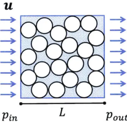
this limit, the grains of sediment pack tightly together forming what is essentially a porous solid. Therefore, (as shown in Figure 2-4) we can determine an expression for fd empirically

with Darcy's law. The steady flow of fluid through the pores of the solid phase will result in a measurable pressure drop across the solid phase. This pressure drop can be related to the inter-phase drag through Equation (2.22).

U

Pin L Pout

Figure 2-4: In a dense mixture (0 -+ 0.65), the viscous drag of the fluid phase on the solid phase can be determined empirically by relating the pressure drop, (pout -Pin) measure over some distance, L, to the measured steady inlet flow velocity, u.

The general method of determining an equation empirically, begins with the plotting of experimental results against dimensionless groups (in this analysis attributed to Blake

[19221). We therefore begin with the empirical relation given in Equation (10) of Carman [1937],

U d 3 _{(Pin Pout) (2.32)}

where u is the measured steady fluid velocity at the inlet (and outlet), k is the permeability of the granular packing, pi, and pout are the measured fluid pressures at the inlet and outlet of the packing, and L is the length of the granular packing (see Figure 2-4). The average pore fluid velocity ue is related to the inlet flow velocity u through Equation (2.29),

U

tie -n

Recognizing that ue is expressible as the difference between the fluid phase velocity and the solid phase velocity, we let,

te ~ Vf - Vs

and assuming that the pressure drop per unit length is approximately uniform, we let, (Pout - _{Pin) - grad(pf)}

L

then Equation (2.32) can be rewritten as,

d2

2

Vf

-

=

d n )2 . grad(pf)

kgo 36(1 - n) or,

grad(pf) = 36k(l _n2-_dd2 2n) 2 0 (vS - Vf) (2.33)

By plugging Equation (2.33) into Equation (2.22), we find

D___ 36k(1 - ri)2r

Pf DL pfg + fd + div(rf) - nd2 (V Vf)

In the steady-state flow considered, and assuming gravitational effects and wall drags are negligible, this becomes

0= fd- 36k(1 - n)271 (VS - Vf)

nd2

or,

fd = 36k(1 - n )211 (Vs - Vf) (2.34)

nd2

Carman gives an average measure for the permeability k of dense packings of spheres

(0.60 < q < 0.647) equal to about 5. Plugging this value into Equation (2.34), we recover the

common expression for fluid drag in soils and sediments, the Carman-Kozeny drag equation (as used in Bandara and Soga 2015]),

fd 180(1 - n)2170 (vS - Vf) (2.35)

nd2

of dense mixtures (0 > 0.6). By observing how measured quantities depend on the

non-dimensional groups describing the flow, a simple formula has been found. However, in the large range of regimes of interest (0 <

#

< 0.65), this expression is still insufficient. Direct

comparison of Equations (2.31) and (2.35) shows that the Carman-Kozeny equation does

not recover the analytical model from the Stokes-Einstein equation. In fact, at low packing

fractions (0 -4 0), the Carman-Kozeny equation under-predicts the drag associated with a

single grain. Although the methodology of presented here is sound, a larger range of packing fractions and flow velocities must be considered in order to form a complete expression for the inter-phase drag.

2.2.3

Simulation Method: van der Hoef's Equation

Determining an expression for the inter-phase drag for the full range of potential packing fractions (0

<

#

<

0.65) has historically been an intractable challenge. Analytical methods

cannot be used for high Reynolds number flows (Re > 1) and flows with non-negligible

packing fractions (# > 0). Experimentally, any loose packing (# < 0.58) without sustained

granular contacts will quickly compact, making the collection of accurate measurements near impossible. In the last 30 years, advances in computational fluid dynamics have made it possible to directly simulate the flows around large clusters of particles immersed in fluid. In particular, we are interested in simulation results that have used the lattice-Boltzman method, a discrete formulation of Navier-Stokes equations which is capable of modeling fluid flows involving complex boundary geometries. van der Hoef et al.

[2005]

and Beetstra et al.

120071 use the lattice-Boltzman method to simulate the flow around mono- and bi-disperse

packings of spheres in the range of 0.10 <

#

< 0.6 and up to Re ~ 1000. As shown in

Figure 2-5, the flow simulation allows the calculation of an average force vector, F. Once normalized, an empirical-like relation can be developed.

U

Figure 2-5: For an arbitrarily dense mixture (0

<

#

<

0.65), the fluid flow around the solid

grains can be simulated using the lattice-Boltzmann method. The resulting average force vector, F, can be normalized and empirically related to the free-stream flow velocity, u.

drags) of each grain, Fi, in the simulated domain, Q,

F = ZFi/N

iEQ

where N is the total number of grains in the domain. To recover the viscous drag component, van der Hoef et al.

[2005]

gives the following definition,

Fd = (1 - #)F

Fd _{is then normalized by the Stokes-Einstein drag from Equation (2.25),}

F = =(I- )F (2.36)

37rlodu 37riodu

where F is the normalized drag force measure and u is the inlet flow velocity of the simulation. Once F is determined for a wide range of simulations, an empirical relation can be developed

by plotting the results against non-dimensional groups and finding a good fit line.

F = F(0, Re)

van der Hoef et al.

[20051

give the following form of F at low Reynolds numbers (Re -4 0),

F(4, 0) -1002 + (1 - #)2(1 -1.5

4#)

(2.37)

(1 -) )0 2

Beetstra et al. [2007] expand on the previous work by considering mono-disperse flows up to Re = 1000 and bi-disperse flows up to Re = 120. The corrected form of F, is then,

0.413 Re (1 - ) -' + 30(1 - 4) + 8.4 Re-0.3 43

F(4, Re) = F(01 0) + 24(1 - 0)2 ( 1 + 1030 Re-(1+40)/2 (2.38)

Now, as in Section 2.2.1, we want to find fd such that,

S-fddv

= Fd

For a sufficiently large domain Q with sufficiently uniform fd,

-fd f dv = Fd

Substituting in Equation (2.36), we find an expression that looks remarkably similar to the expression in Equation (2.27),

Recalling the definitions in Equations (2.28), (2.29), and (2.30), we arrive at the final ex-pression for the inter-phase drag fd

180(1 - 0),qo

fd = d2 - F(#, Re) - (v, - vf) (2.39)

where F(#, Re) is given as in Equation (2.37) or (2.38). Since this expression derives from direct simulation of flows through a wide range of granular packings, we expect it to more accurately represent the inter-phase drag of the mixture than either Equation (2.31) or (2.35).

2.2.4

Comparison of Methods

As shown in Figure 2-6, Equations (2.37) and (2.38) have properties which will be useful in the simulation of our continuum. First, both expressions return finite values for packing fractions in the range 0 < q < 1 and Reynolds numbers in the range Re > 0. Although physically we do not expect packing fractions above ~_ 0.65, it is possible that the contin-uum representation could exceed this limit. In the dilute (# -+ 0), low Reynolds (Re -> 0) limit, Equation (2.38) reduces to Equation (2.38) with the final result,

F(0, 0) = 1

Plugging this into Equation (2.39), we recover the Stokes-Einstein inter-phase drag from Section 2.2.1,

180(1 - 0)710 18n(I - n)77o

fd= d2 .(VS - Vf) 1nd2 .(vs Vf)

In the dense (# -+ 1), low Reynolds (Re -+ 0) limit, Equation (2.38) reduces to Equation (2.38) with the final result,

100

F(1, 0) ~102 ' (1 --q) 2

Plugging this into Equation (2.39), we recover the Carman-Kozeny inter-phase drag from

Section 2.2.2,

18002710 180(1 - n)2

.

-(1 - O)d2 .id 2

2.3

Material Constitutive Models

In this section, we lay out the thermodynamic rules governing the behavior of the mixture.

When considering a single phase of material, it is often useful to assume that internal energy

(E), entropy (rI), and absolute temperature

(9)

are basic properties of a material. That is, they do not need to be defined in terms of other more basic properties. For this analysis, we assume that analogous continuum fields exist describing the energy, entropy, and temperature

106 10 5 10 4 Q 02 101 10 0 0 0.1 0.2 0.3 0.4 0.5 0.6 0.7 0.8 0.9

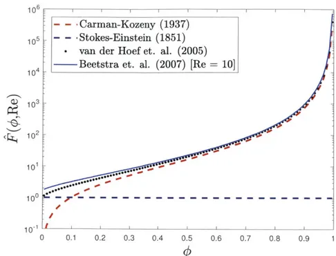
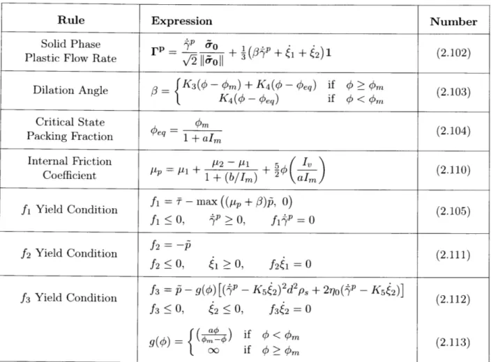
Figure 2-6: Comparison of the normalized drag force expressions, F(O, Re). In the dilute limit (0 -÷ 0), the Carman-Kozeny equation clearly under-predicts the analytical drag force

given by the Stokes-Einstein drag equation. In the dense limit (0 - 0.65), the

Stokes-Einstein drag equation under-predicts the experimentally derived Carman-Kozeny equation. The expressions from van der Hoef et al.

[20051

and Beetstra et al. 12007] capture both limits correctly.

of the two continuum phases; however, as stated by Wilmanski

[2008]

and Klika

[2014],

the physical basis of these fields is poorly defined. We therefore rely on the intuition developed in Gurtin et al.

[2010]

to develop the governing thermodynamic laws of the continuum mixture. Then, through careful consideration of microscopic flow behavior, experimental observations, and the results of particle simulations, we develop the constitutive laws governing the phase stresses in Equations (2.17) and (2.18). In Section 3, we verify that these relations recover the empirical limiting behaviors of fluid-sediment mixtures. For this formulation, we return to the continuum representation of the mixture shown in Figure 2-2. In particular, we are interested in the behavior of a part of the mixture defined by a volume Q.

2.3.1

First Law of Thermodynamics

The first law of thermodynamics states that the rate of change of the total energy stored within a volume must be equal to the rate of heat flow into the volume plus the external

power exerted on the volume. The total energy stored within a volume is the sum of internal energy and kinetic energy. We consider the part of the solid body defined by the volume Q,

- - Carman-Kozeny (1937) -Stokes-Einstein (1851)

van der Hoef et. al. (2005) Beetstra et. al. (2007) [Re = 10]

---I0 1

1

and we express the conservation of energy of this part as follows,

Ds (s(Q) ₊

Dt

KS(Q))

- QS(Q) +

W()

- Qi(Q) - WVi() (2.40)

where,

e Ss(Q) is the internal energy of the solid part.

* Is(Q) is the kinetic energy of the solid part.

" Qs(Q) is the external heat flow into the solid part.

* IN, (Q) is the external power exerted on the solid part.

" Qj(Q) is the inter-phase heat flow from the solid part to fluid part (defined by the volume Q).

" Wi(Q) is the inter-phase work power exerted on the fluid part by the solid part. We also consider the part of the fluid body defined by the volume Q and express energy conservation of this part similarly,

+

Kf(Q))

=

Qf()

+

W4f( ) +

Qi(Q)

+Wi)

(2.41)

where,

" Ef(Q) is the internal energy of the fluid part. " Ikf(Q) is the kinetic energy of the fluid part.

" Qf(Q) is the external heat flow into the fluid part.

" Wf(Q) is the external power exerted on the fluid part.

Summing the expressions for phase-wise energy conservation in Equations (2.40) and (2.41), we arrive at the expression for the combined conservation of energy in

volume, ,

the mixed

Dt (

CS

_{(Q) )}

D + f (Q)) = Qs(Q) + Qf (Q) + Ws (Q) + Wf (Q) (2.42)

We let the internal energies, Es(Q) and Ef(Q), be defined by integrating the specific internal

energies, Es and Ef over the volume Q,

(Es() = PsEsdv ef() j pfEfdV

(2.43) Dt

We let the kinetic energies, Ks(Q) and Kj(Q), be similarly defined by integrating the specific

kinetic energies over the volume Q,

IsCS Q) = P -(VS .VS) dv

= 2

(2.44) Cf(Q)= Ip (v vf)dv

The external heat flows, Qs(Q) and Qf(Q), are characterized by the phase-wise external heat

fluxes, q, and qf, at the boundary DQ and phase-wise internal heat generation, q, and qf,

within the volume Q as follows,

Q() = -f (q n)da + qsdv

(2.45)

Qf(Q) =-j (q n)da + qfdv

We also define an inter-phase heat flow, Qj(Q), in terms of the inter-phase heat transfer, qj (volume averaged heat transfer from the solid phase to the fluid phase),

Qi() = I qidv (2.46)

For the external powers, WlVs(Q) and /VfW(Q), we return to the definition of the phase stresses in Equation (2.4) and the expression for external body forces in Equation (2.3) to define,

WS() =

f

(o-,n- v)da +

f

(psg -v)dv

.ID~ JQ(2.47)

/Vf ()

J

(on- vf)da + j (pf g- vs)dv

To simplify the analysis of the combined conservation of energy in Equation (2.42), we will apply the definitions given above to each term individually, then recombine all the terms at the end. This will allow us to cleanly derive an integral expression for the combined conservation of energy within a mixed volume Q. We begin this analysis with the first term, the time rate of change of the total energy stored in the solid part defined by the volume Q. Using the relations for internal and kinetic energies from Equations (2.43) and (2.44), we can rewrite this term as,

Applying Reynolds' transport relation, we find,

j

[

S

((Es + (vs - V)) + PS (ES + (vs vs)) div(vs)1 dv

which is equivalent to,

J

Dsp[( d(v>

ES

+

+

P)

DS + 1

S

i

f [ Dt +PsdV~Vs)

(

2 Dt 5 + V(v5)) vD) dv

Using the expression for solid phase mass conservation from Equation (2.7), we get the final integral form for the rate of change of total energy in the solid part,

D ( (Q)+ ()

j

(S DQ) + S D -S dv (2.48)

A similar analysis can be performed for the expression of material rate of change for the total energy in the fluid part defined by the volume Q (the second term in Equation (2.42)); the result is given here,

Dt ( " Dt Dt vfd2.

Keeping these relations in mind, we continue through the terms in the combined ex-pression for conservation of energy. The first and second terms on the right hand side of Equation (2.42) we recognize as the external power acting on the mixed volume Q. Applying the definitions from Equation (2.47) to these terms, we find that,

/VV(Q) + )Wf () =

j

(on -v. + ofn -vf)da +

j

(isg -vs + pfg -vf)dv

Applying the divergence theorem to the above expression, we find the final integral form for the combined external power acting on the volume Q.

W)(Q) A+ )V1() =

f

[(div(a,) + js g) - vs + (div(of) + pf g) - vf] dv

(2.50) +

j

[a

: grad(v) + o : grad(vf)] dv

Lastly, we consider the third and fourth terms on the right hand side of Equation (2.42). These are the expressions for the external heat flow into the mixed volume Q. Applying the definitions from Equation (2.45) to these terms, we find that,

Applying the divergence theorem to the above expression, we arrive at the final integral form for the combined heat flow into the volume Q.

Qs(Q)+Q(Q) = (- div(q + qf) + q + qf)dv (2.51)

Substituting in the phase-wise energy conservation expressions from Equations (2.40), (2.41),

(2.50), and (2.51) into the combined energy conservation expression in Equation (2.42), we

find the integral form of the combined conservation of energy in the mixture,

f (

D + Pf Df + -f D 'v v + Vf D v f) dv = ((div(a ,) + ps g) -v ,,) d v + ((div(of ) + pf g) -vf) dv + as : grad(vs)dv + j : grad(vf)dv + (qs + qf - div(qs + qf)) dv (2.52)

Since this expression must hold for any choice of volume Q, the strong form must also be true. From here, we continue our analysis without the need for pesky integral expressions.

_ DsE DfEf Dsvs - Dfvf

Dt Dt +j5 D Vs+Pf Dt -vf=(div(7)+pg)-v6

+ (div(of ) + pf g) -vf

+ a. : grad(v,) + af : grad(vf)

+ qs + qf - div(qs + qf)

By momentum balance in Equation (2.16) and the definition of the buoyant term in Equation

(2.20), this is equivalent to

-Ds

DfEf Ps Dt PfDt =pf grad(n) - (vs - vf) + fd (vs - Vf) + a, grad(vs) + 0f : grad(vf) + q8 + qf - div(q. + qf)

Substituting in the expressions for the specific form of the phase stresses in Equations (2.17),

energy in the mixture,

_s Dtf _ D P5 n Dfp

SDt Dt p Dt

+ fd (v. - Vf) (2.53)

+ & grad(v,) + -rf : grad(vr) + qs + qf - div(qs + qf)

2.3.2

Second Law of Thermodynamics

The second law of thermodynamics states that the rate of change of the total entropy within a volume Q must always be greater than or equal to the combined entropy flow into the volume. Drumheller [2000] gives the following necessary condition for entropy imbalance of a mixed volume Q,

Dt( Dt J() - f() ;> 0 (2.54)

We add two additional conditions by considering the entropy flow into the part of the solid body defined by the volume Q,

DS(Q)- _{isJ() + Jis() ;> 0}

(2.55)

Dt

and the entropy flow into the fluid of the solid body defined by the volume Q, DfSf-(Q) _{i() - Jf() ;> 0}

(2.56)

Dt

where,

" S₈(Q) is the entropy of the solid part.

" Js(Q) is the external entropy flow into the solid part.

" Sf(Q) is the entropy of the fluid part.

" Jf(Q) is the external entropy flow into the fluid part.

* Ji,(Q) is the inter-phase solid entropy flow due to heat flowing from the solid part

into fluid part (defined by the volume Q).

* Jif(Q) is the inter-phase fluid entropy flow due to the heat flow into the fluid part

from solid part.

Together, Equations (2.54), (2.55), and (2.56) give the necessary and sufficient conditions for satisfying the second law of thermodynamics within a mixed volume Q. We now define

the integral forms of the terms in these expressions. We let the total entropies, S,(Q) and

Sf(Q), within a volume Q be defined in terms of the phase-wise specific entropies, YS and qf,

SSs(A)fjtisydv

(2.57)

Sf() = pf/f dv

The first term in Equation (2.54) can be rewritten with the definition for the solid phase entropy in Equation (2.57) as follows,

DSSs

(Q)

Dt

DS

- Dt jQ PSIsd Using Reynolds' transport relation,

DSS (Q) Dt

Ds

SDt (psTys) + gsqs div(vs) IdA

which, by solid phase mass conservation in Equation (2.7), is equivalent to

DsS,()

f

Dt Ja Dt

By similarity, the second term in Equation (2.54) is equivalently,

Df Sf()

Dt { DLnfaD o (2.59)

We let the external entropy flows, Js(Q) and Jf(Q), into the volume Q be given as follows, -. n da +

(qf

- n da

+

4dv

d which, by the divergence theorem, are equivalent to,

f () =

-J

/

div

j[div

qs

()--dv

q

(-)

- f]dv

where ds > 0 and i5 > 0 are the phase-wise absolute temperatures.

Unlike the inter-phase heat flow, Qj, which represents the heat flow out of the solid phase

(2.58)

J8(Q) =

-is(