A set of programs for analysis of kinetic and equilibrium data

A set of programs for analysis of kinetic and

equilibrium data

Marc Eberhard

Abstract

A program package that can be used for analysis of a wide range of kinetic and equilibrium data is described. The four programs were written in Turbo Pascal and run on PC, XT, AT and compatibles. The first of the programs allows the user to fit data with 16 predefined and one user-defined function, using two different non-linear least-squares procedures. Two additional programs are used to test both the evaluation of model functions and the least-squares fits. One of these programs uses

two simple procedures to generate a Gaussian-distributed random variable that is used to simulate the experimental error of measurements. The last program simulates kinetics described by differential equations that cannot be solved analytically, using numerical integration. This program helps the user to judge the validity of steady-state assumptions or treatment of kinetic measurements as relaxations.

Introduction

To analyse kinetic and equilibrium measurements, it is very often useful to reduce the experimental data to a model that is described by only few parameters and free of experimental errors. This reduction can be achieved most conveniently by fitting data to a model curve using least-squares procedures. Here, a set of programs is described to fit model curves to experimental data, to simulate measurements that are based on a model curve and to simulate kinetic transients.

Many of the commercially available fit programs provide anlaytical model functions that are in many cases not appropriate for fitting kinetic and equilibrium data. For this reason it was decided to write the program COSY, which offers useful analytical model functions and four variants of progress curves of enzymatically catalysed reactions. These transients have to be evaluated iteratively since they do not have analytical solutions. Additionally, COSY allows the user to define his or her own model functions. Since our experience shows that, in practice, only a small subset of all possible model functions is used, the most important models are provided as predefined functions. An additional motivation to write COSY was to combine algorithms useful for fitting experimental data,

Biozentrum, University Basel, Department of Biophysical Chemistry, Klingelbergstrasse 70, CH-4056 Basel, Switzerland

estimating errors and finding criteria for selecting one particular model.

It is important to find conditions that allow an unambiguous assignment of one particular set of data to one particular model function. These conditions usually involve a low experimental error and a suitable range of the measurements such that the data exhibit features characteristic for one model function. It is often misleading to take the model function that fits the experimental data with the lowest sum of squared deviations (Duggleby and Nash, 1989), because model functions with many parameters tend to fit experimental data better than those with few parameters. Furthermore there is no straightforward way to give confidence limits on parameters of non-linear models (Press et al., 1989). For these two reasons a second program, SYNDAT, was written. SYNDAT calculates curves from a model function given by the user, and introduces normally distributed errors. The calculated curves are then fitted in order to assess the precision with which the original parameters are reproduced. Alternatively, the curves may be fitted to model functions different from the original one, in order to judge whether the data can be unambiguously assigned to one model. COSY and SYNDAT provide three goodness-of-fit criteria, a x square, a signed rank and a runs test.

The utility MODFUN is used to assess the precision with which model functions and their derivatives are evaluated with respect to the fit parameters.

The simulation of enzymatic kinetics has been found to be very useful to judge the validity of the steady-state assumption. Simulations of mechanisms of binding may resolve discrepan-cies among experimental data (e.g. Wang, 1985) and find conditions for useful simplifications. For these reasons SIMKIN, a program that simulates six different kinetic mechanisms, has been included in the present package. Since a fourth-order Runge-Kutta procedure (Press et al., 1989) was found to give the most accurate results (among four one-step and predictor-corrector methods) when applied to kinetics with analytical solution, this algorithm is applied in SIMKIN.

Attempts have been made to introduce simulations as model functions into COSY, but the simulations together with the least-squares fit procedure are too time consuming and contain too many parameters to be conveniently applied. It is a better strategy to analyse complex kinetics by simulations and thereby evaluate conditions for useful simplifications. For example, kinetics may be simplified by using initial concentrations near

the thermodynamic equilibrium, such that the perturbations of higher orders can be neglected (Hiromi, 1979). The transients generated by SIMKIN may be analyzed with COSY.

The programs described here have been successfully applied in our laboratory for the analysis of enzyme kinetics, stopped-flow kinetics (Eberhard and Erne, 1989) and protein folding experiments (Herold and Kirschner, 1990).

System and methods

Hardware requirements

The programs were developed on a TWTX 88-XT equipped with a 8087 numeric coprocessor, 640 kbyte RAM, Hercules monochrome graphics, a 20 Mbyte hard disk and two floppy drives. The minimal configuration is a PC or compatible with 512 kbyte RAM, one floppy drive and Hercules, CGA, EGA or VGA graphics. All four programs described were success-fully tested on a TWIX 286-AT, TWIX 386-AT, and HP vectra ES/12, all with EGA or VGA graphics, but without numerical coprocessor.

Software requirements

MS-DOS or PC-DOS version 2.0 or later may be used as the operating system. The programs were developed under MS-DOS version 3.20. The programs were written in Turbo Pascal version 4.0, released on June 1987 (Borland Inc.). Apart from MS-DOS or PC-DOS, no further software is required to run the four programs (COSY, SYNDAT, MODFUN and SIMKIN). The Turbo Pascal command line compiler (TPC.EXE, available from Borland Inc.) is required to introduce self-defined model functions and kinetic mechanisms. Since COSY, SYNDAT, MODFUN and SIMKIN provide all definitions required, no programming experience is required. The ASCII files and the installation files may be processed with a text program.

Algorithms

Two non-linear least-squares algorithms have been inroduced into COSY: the Marquardt procedure (Marquardt, 1963) and the ELORMA procedure (Gampp et al, 1980). Both procedures use initial parameters estimated by the user to evaluate the model function and to refine the fit parameters. While the Marquardt procedure refines each of the fit parameters, the ELORMA procedure first eliminates the linear parameters from the model function and only fits the non-linear ones. In this way the number of parameters to be refined is reduced and convergence is achieved faster, in particular if the correlation between linear and non-linear parameters is high (Gampp et al., 1980). In COSY, both fit algorithms need approximately the same time for one iteration, but ELORMA requires usually fewer cycles to converge. Otherwise the two algorithms are equivalent. COSY, SYNDAT and MODFUN apply the Newton-Raphson

procedure to evaluate the steady-state progress of an enzymatically catalysed reaction and its derivative with respect to the fit parameters (Duggleby and Morrison, 1977; Press et

al, 1989). x 0 c • (T 0 L 2 3 Deviation -3 -2 -1 2 3 Deviation

Fig. 1. Comparison of the Gaussian curve with its model approximation. X-axis in a (standard deviation) units, X-axis in arbitrary unit. (A) Frequency histogram of 6000 random numbers calculated with the approximation function. The smooth curve represents the predicted distribution of a normal deviate. (B) Frequency histogram of 6000 random deviates obtained with die Box-Muller algorithm. The smooth curve is the distribution of a normal deviate. (C) The Guassian density function (solid curve) predicts the distribution of a random variable calculated with the Box-Muller procedure. The dashed curve predicts the distribution of a random variable obtained with the approximate function.

SYNDAT and SIMKIN each apply two different algorithms that produce normal deviates. The idea behind the first approach is that the integrated form of the normal frequency curve can be used to transform uniform deviates into Gaussian ones. Since the integral of the normal frequency cannot be obtained in analytical form, a function that approximates it is used (Barlow,

1985):

fix) = (expt(jtV8/Il)/ff] - l)/2{exp[(jcV8/Il)/ff] + 1) fix) approximates the integrated Gaussian density function

reasonably well (Figure 1C). The reverse function

xif) = aVn/8) ln[(l + 2/)/(l - 2/)]

produces approximately normally distributed values x(f) from uniformly distributed random numbers/(f being between - 0 . 5 and +0.5). The approximated density function is slightly sharper than the Gaussian curve but becomes broader at low density. Therefore the approximated random variable yields more frequently values with large deviations than a normal random variable.

The second algorithm uses the Box-Muller procedure as described by Press et al. (1989). A comparison of the two procedures is presented in Figure 1. Both SYNDAT and SIMKIN uses two sources of uniform deviates, either the random number generator provided by Turbo Pascal version 4.0 or one based on a subtractive method (termed ran3 in Press

et al., 1989), as specified by the user. The first source is about

five times faster than the second but produces deviates that have a higher recurrence.

The fourth-order Runge-Kutta method is applied in SIMKIN to simulate kinetic mechanisms, as described by Press et al. (1989).

Implementation

Data format and input/output

All the four programs use the same data format: a record of up to 100 pairs of reals (for experimental or simulated data), 16 real parameters and 16 integer parameters. Up to 10 records can be handled simultaneously. The records can be transformed to ASCII format and back to binary format. All four programs allow redirection of the output to various devices (printer, files, serial ports). Additionally, each of the programs provides an MS-DOS shell, i.e. they allow the user to switch to the operating system during program execution without losing any data. In this way, MODFUN, SYNDAT and SIMKIN or any other program can be called and executed within COSY, MODFUN, SYNDAT or SIMKIN. Each of the programs uses two configuration files: the first is used by all four programs of the package and contains control sequences for both matrix printers

and plotters and the setup of the graphics. The second type of configuration file is specific for each of the programs and contains default paths and specifications of algorithms, e.g. whether the Box—Muller or the approximate method is used to produce random deviates.

COSY offers an interface section which allows the user to call any other program. It differs from the MS-DOS shell mentioned above in that the foreign programs can be selected from a menu rather than by typing MS-DOS commands. The user specifies three lines for each of the programs in the configuration file of COSY. The first line contains the filename of the program to be executed, the second the entry that appears in the menu of COSY. The third line may specify an ASCII file that contains data to be transferred from the foreign program to COSY. In order to be correctly read the ASCII file should contain a table with a variable in one column and a measured value in a second. This option couples COSY to other programs that are involved in data acquisition and processing.

Model functions

COSY, MODFUN and SYNDAT offer the following 17 model functions:

1. Exponential function (one, two or three overlapping ex-ponentials).

2. Progress of an enzymatically catalysed single-substrate reaction under steady-state conditions (substrate or product concentration versus time).

3. As model 2 but including competitive product inhibition (substrate or product concentration versus time: Duggleby and Morrison, 1977).

4. Progress of an enzymatically catalysed Bi-Bi-ping-pong reaction under steady-state conditions. One of the substrates is assumed to be held at constant concentration by recycling of its product, according to Duggleby and Morrison (1978). 5. As model 4 but without the assumption of one substrate

to be present at constant level.

6. Steady-state kinetics (Briggs-Haldane kinetics, initial velocity versus substrate concentration).

7. Co-operative steady-state kinetics (all-or-none model, initial velocity versus substrate concentration).

8. Binding at equilibrium involving two components (signal versus total ligand concentration).

9. Kinetics of binding involving two components, treatment as single-step relaxation (observed rate constant versus total ligand concentration).

10. Binding at equilibrium involving three component (two components that compete for binding a third species; signal versus total concentration of the third species).

11. Binding at equilibrium involving three component (as model 10, but signal versus total concentration of one of the competing components).

single-step relaxation (two components that compete for binding a third species; observed rate constant versus total concentration of the third species).

13. As model 12 but observed rate constant versus total concentration of one of the binding components. 14. Titration of a signal with two pKa (signal versus pH).

15. Folding at equilibrium (signal versus concentration of a denaturant).

16. Spline interpolation (for any kind of data). 17. Function specified by the user.

Models 1 - 7 deal with steady-state enzyme kinetics, 8 - 1 3 with binding phenomena.

The Newton-Raphson algorithm (Duggleby and Morrison, 1977) is implemented in COSY, SYNDAT and MODFUN to evaluate the progress of enzymatically catalysed reaction, model functions 2—5. Models 2 and 3 are also useful to determine the initial velocity of enzymatically catalysed reactions that show curved transients. In these cases it is difficult to obtain reliable initial velocities from linear regression.

Models 10 and 11 allow one to assign a signal component to each of the five species (three monomers and two complexes). Model 10 may also be used to analyse binding of a ligand to a molecule with two different binding sites. Non-specific binding, which is often encountered when analysing binding properties, may be treated in this way.

Models 9, 12 and 13 treat the system as a single-step relaxation, assuming it to be near the final equilibrium (Hiromi, 1978). Models 12 and 13 assume that the interaction of the ligand with one of the two binding components is faster than that with the other. Conditions for this useful approximation may be evaluated by simulation, using SIMKIN. A possible application of models 12 and 13 is to couple the interaction of an indicator with a ligand to the interaction of ligand with protein (Hiromi, 1979).

Model 15 describes a system of two, three or four states of a protein: one native, up to two intermediates, and one denatured state. A contribution to the total signal of each of the four states is specified by the user. Since they are usually not known, the contribution of the intermediates to the total signal can be included as a fit parameter. The basis of this model is the observation that the free energy of unfolding of proteins in the presence of urea or guanidinium hydrochloride is linearly related to the concentration of denaturant (Pace, 1986). The free energy of conversion of one state into the next is also assumed to be a linear function of denaturant concentration. In the simplest case, with one native and one denatured state, the free energy of unfolding under physiological conditions may be evaluated. Model 16 is useful to represent spectra, elution diagrams or any data that cannot be described by a model curve.

COSY, MODFUN and SYNDAT allow the user to define further model functions (model 17). First, the programs ask

for a title of the new function and for names of each of the parameters. Up to 15 parameters may be specified. Then the user is requested to specify a model function which may include iterative procedures, local variables but no input/output commands such as 'read' and 'write'. The programs (COSY, MODFUN and SYNDAT) will convert the algorithm given by the user into a Pascal source code and compile it by using the Turbo Pascal command line compiler. The resulting program code is appended to the data file. Therefore each data set may be equipped with its own model function or procedure. The size of the program code must not exceed a certain limit (8000 bytes by default). The number of the user-defined function, 17, merely causes the programs, upon loading a data set, to look for the model function in the data file rather than in its internal list of predefined functions. Once loaded, a user-defined model function is kept in the memory (RAM) to ensure optimal speed of execution. The Turbo Pascal command line compiler (TPC.EXE, commercially available from Borland Inc.) is required for introducing new model functions.

Program 1: COSY

COSY is the most powerful and flexible of the four programs. The most important features are the following:

• Each of the parameters of a model function can be defined either as fit parameter or as constant parameter. In this way the user decides which parameters are to be refined by the fit procedures.

• Experimental error of the input data can be accounted for in three ways. The user may (i) specify the error of each of the values, (ii) assume the error to be the same for all data or (iii) specify the error to be a linear function of the input data. In any case, errors are given as standard deviations. The input data are weighted with the reciprocal variance (the variance is the square of the standard deviation). By default, all standard deviations are set to unity. • COSY provides three goodness-of-fit criteria which are all applied to the residuals (difference between observed and predicted values). A ranks order test, also known as Wilcoxon's signed rank test, and a runs test are used to judge whether the median of the residuals equal zero and whether the residuals are drawn at random from a single population respectively (Ostle and Mensing, 1975). A x-squared test applied to the frequency of the residuals estimates the probability that the residuals are normal deviates. These tests provide a basis to evaluate the appropriate model function (Atkins, 1976). In addition, the fit procedures calculate a X square due to the experimental values, which measures the closeness of the predicted and experimentally determined data, and the covariance matrix, which is used to estimate the standard deviations of each of the fit parameters

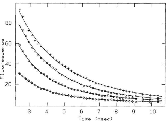
Table I. Example of a least-squares fit Temperature (°C) k2 (s"1) X square (data) X square (dist) (P) Rank test (P) Run test (P) 20.4 545.2(78) 209.5(24) 0.016 24.8 0.001 2218 0.68 32 0.0004 25.4 525.7(46) 172.3(37) 0.256 13.3 0.05 2162 0.55 44 0.2090 3 0 0 678.1(64) 177.4(32) 0.168 17.4 0.01 2050 0.31 35 0.0042 39.2 670.2(73) 108.5(44) 0.072 2.34 >0.05 2006 0.24 41 0.0808

The first halves of the measured curves are shown in Figure 2. ky and k2 denote

the rate constants of the two overlapping exponentials. Standard deviations are given in brackets, x square (data) denotes t(Y0 - ^J2/^ where Yo and Yp

refer to the observed and predicted values respectively. The measured data consist of 96 values. The test quantity of three statistical tests on residuals are evaluated by COSY and SYNDAT. x square (dist) denotes L(F0 - F^IFp where Fo

and Fp refer to the observed and predicted frequencies of the residuals

respec-tively. F. is a normal deviate. (P) denotes the approximate significance level.

(assuming normally distributed errors of the fit parameters). An example is presented in Table I. Upon request, COSY writes the residuals into a text file to allow further treatment with other programs.

• Both the Marquardt and the ELORMA fit procedures can be run with two different iteration protocols. In the first one the user is asked after each iteration whether to continue or to leave. In the second mode, COSY iterates automatically until convergence is achieved, i.e. until the sum of squared residuals changes by < 10~6 upon further iterations [the

sum of squared residuals is defined as Efvalue(observed) - value(modell2, cf. Duggleby and Nash, 1989]. If

convergence is not achieved within a certain number of iterations, which is related to the number of parameters to be fitted, COSY stops and gives a message. In any of the three modes, each of the fit parameters, their changes upon the next iteration and the sum of squares residuals are shown after each iteration. The automatic iteration procedure may be interrupted by the user.

• A variety of operations can be applied to whole data sets, either operations with one operand, like differentiation, integration and transformation to Scatchard representation, or transformations with several operands, such as addition and subtraction.

• Up to 10 curves may be displayed simultaneously. Any section of the graph may be enlarged to show details. The graph can be plotted on a HP plotter interfaced to an RS-232 port of the PC. (Figures 2 and 3 were obtained in this way, using a HP 7221A plotter.) Plots can be redirected to files. Hard-copies can be made on matrix printer.

In the current version of COSY the ELORMA algorithm is applied only to the exponential functions (models 1 - 3 ) while the Marquardt procedure can be applied to any of the model

functions. The fit procedures usually converge to the best fi' with few iterations ( 4 - 6 ) if no more than three fit parameters are included and if the initial parameters do not deviate by more than a factor of two from their final values. Even when the initial parameters deviate by orders of magnitude, convergence is often achieved after some 10 iterations. If more than five fit parameters are included, convergence problems may arise, in particular when the parameters are coupled to each other. On a PC-XT compatible with numeric coprocessor, one individual iteration is performed within < 1 s, with the exception of model 15 (cf. previous section). Therefore, in most cases, a set of experimental data is fitted within a few seconds.

The choice of the appropriate model function is straight-forward if it has a physical basis. It was found that the decision between the variants of the exponential function and those of the protein folding model is particularly difficult, for two reasons. Usually there is no physical reason to favour one variant over the other, and the model curve with the most parameters is normally the one that gives the best fit. As a general rule, the model with the fewest parameters that still produces a satisfactory fit should be selected. As an example, the result of stopped-flow experiments of CA2+ binding to a

fluorescent Ca2+ indicator is shown in Figure 2 and Table I.

In this case, residuals are normally distributed at a significance level of 5 %, except those of the data set obtained at 20°C. The number of runs is generally lower than expected (in the present case, 48 runs are expected), suggesting that the residuals exhibit serial correlations.

The decision whether to include competitive product inhibi-tion into the progress of an enzyme-catalysed reacinhibi-tion is straightforward for the single-substrate mechanism, because with the wrong model progress curves show systematic deviations. A a consequence the number of runs in % residuals may be as low as five rather than the 48 expected if the residuals are random. According to our experience the progress curves of the Bi-Bi mechanism (models 12 and 13) should be applied with caution. The reason is that Bi-Bi-ping-pong mechanisms with very different parameters, i.e. inhibition constants, produce progress curves of similar shape. The analysis of such progress curves is justified only if experimental errors are low and if there is independent support for a Bi-Bi mechanism (see, for example, Klotz and Hunston, 1984).

Program 2: MODFUN

This program evaluates and displays the value of any of the 17 model functions and their derivatives with respect to the fit parameters, for a given argument. The user selects one of the model functions, sets the parameters to the desired values and specifies one or several value of the variable. In this way, the result of a model function may be verified, which is useful to estimate initial fit parameters. MODFUN may be called from

6 7 8

Time (msec)

10

Figs 2. Application of COSY. Temperature dependence of the dissociation of a Ca2+-indicator complex, measured by stopped-flow fluorescence (Eberhard

and Erne, 1989). One micromole of the fluorescent Ca2+ indicator Fluo-3 (Minta et al., 1989) saturated with Ca2 + was mixed with 10 mM EGTA [ethylenebis(oxyethylenenitrilo)tetra-acetic acid] and the decrease of fluorescence emission above 495 nm observed (excitation at 470 nm). The experiments were performed in 50 mM HEPES [2-(4-2-hydroxyl)-1 piperazinyl)-ethanesulfonjc acid], 150 mM NaCl, pH 7.0. The transients were fitted to two overlapping exponentials, using COSY. The result of the Marquardt fit is presented in Table I. The symbols are the following: + (20.4°C), x (25.4°C), • (30.0°C), o (39.2°C). The transients start at 2.4 ms due to the dead-time of the stopped-flow instrument.

COSY since all the programs are equipped with an interface to MS-DOS.

Program 3: SYNDAT

SYNDAT is used to evaluate confidence limits of the parameters of model functions by Monte Carlo simulation in the following way. The user selects a model function, specifies all the parameters, the number of data to be generated, the range of the data on the abscissa, and a standard deviation, assuming the data to have normal deviates (see below). SYNDAT calculates up to 2048 data sets, each of which contain values that are scattered around the model function. If the user tells SYNDAT to produce > 10 data sets, the program fits each of the data sets automatically and saves only the fit parameters, otherwise the whole data sets are saved. If convergence cannot be achieved, SYNDAT writes a message to the output file.

Subsequently the distribution of each of the fit parameters is analysed, in one dimension. Since the output files have ASCII format, other programs may be used to analyse the whole

Table D. Monte Carlo simulation of progress curves performed with SYNDAT

Data set Initial model 1 2 3 4 5 6 7 8 9 10 Mean Standard deviation Fit parameter y mix 20 20.176316 20.485252 19.348404 20.004785 20.105892 19.776956 19.739686 20.008679 19.809770 20.015587 19.947133 0.303395 450 450.464388 447.402295 451.499968 448.960495 449.987801 450.010470 451.241196 450.838957 451.973546 448.452075 450.085345 1.439206 600 560.608905 528.403395 717.382651 609.023680 579.326085 644.104495 639.517936 590.260840 618.557794 611.780048 609.896473 51.715996

parameter space. SYNDAT gives one-dimensional confidence limits and a standard deviation for each parameter to be analysed. Calculation of one data set from a simple model

c

8

u

100

80

60

20

-300

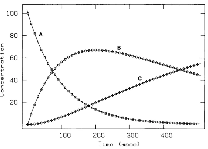
Fig. 3. Reliability of numerical integration. The simulation of a two step irreversible reaction was carried out with SIMKIN with the following parameters: <fc, = 10 s~' (rate constant of A — B); k2 = 2 s"1 (rate constant of B — C); [A], = 100, [B], = 0, [C], = 0 (initial concentrations). Numerical integration was

performed with 0.001 s steps, from 0 to 0.5 s, using the fourth-order Runge-Kutta algorithm. Every 0.01 s the actual concentrations of A, B and C were saved and plotted versus time. The solid curves represent the analytical solutions. Under the above conditions, the numerical solution deviates from the analytical one by < 1 0 "9.

function, e.g. a single exponential described by three parameters, and the fit of the data set take - 2 - 4 s (SYNDAT run on a 8 MHz PC-XT compatible with numeric coprocessor). In order to obtain a statistically significant distribution of the fit parameters, some 1000 data sets have to be calculated and fitted.

As mentioned above, SYNDAT introduces normally distributed random deviates into the calculated data. The standard deviation of the deviates is assumed to be a linear function of the calculated data. Therefore SYNDAT asks for an offset and a proportionality factor that relates the data to their standard deviations. The rationale of this feature is that most experimental data are obtained by subtraction of some sort of baseline from the proper data. Therefore, experimental error is introduced not only by the measurement, but also from the baseline. The errors of the baseline are accounted for by a constant standard deviation, while the experimental error is assumed to be proportional to the measured value. The algorithm that generates approximately Gaussian deviates

produces — 105 random numbers per second when run on a XT compatible without numerical coprocessor, and ~ 1900 per second with numerical coprocessor. Under the same conditions, the Box-Muller method produces 105 and 1620 numbers per second. Thus, the approximate functions has the advantage of being slightly faster than the Box — Muller algorithm when run on a computer with numerical coprocessor support. On the other hand the Box-Muller procedure produces true normal deviates. A summary of an output file generated by SYNDAT is shown in Table II. In this example 10 progress curves of enzyme-catalysed reactions, with competitive product inhibition, were generated by SYNDAT, each from t = 0 - 1 2 0 s, using [S]j = 600 (initial substrate concentration); [P]j = 40 (initial product concentration). The experimental error was simulated with the approximate function (see previous section) using a standard deviation offset of 6 and a proportionality factor of 0.001 (i.e. a value of 500 is associated with a standard deviation of 6.5). SYNDAT fits the 10 transients automatically and writes the result to a text file, from which the table was compiled.

Between three and five iterations were required to achieve convergence of the three fit parameters. Table II reveals that

Km is reproduced accurately, whereas Kp fluctuates

considerably, indicating that Kp is sensitive to experimental

error.

Program 4: S1MKIN

SIMKIN allows the simulation of seven mechanisms:

1. Kinetics of binding involving three components (two components that compete for binding to a third species). 2. Kinetics of binding involving four components (three components that compete for binding to a fourth species). 3. Kinetics of binding involving five components (four components that compete for binding to a fifth species). 4. Kinetics of binding involving three components (two components that compete for binding of a ligand; one of the binding components is assumed to bind successively four ligand molecules, each with different rate constants). 5. One-substrate kinetic mechanism of an enzymatically catalysed process (five enzyme species: free enzyme, two different substrate complexes, an enzyme-transition state complex, and an enzyme —product complex).

6. Same as 3 but with the second enzyme-substrate complex as a branch rather than on the reactive pathway (non-productive binding).

7. Kinetic mechanism defined by the user.

If some of the rate constants are set to zero or if various components are used in large excess, a wide variety of kinetic mechanisms can be simulated. In addition, SIMKIN allows the user to specify kinetic mechanisms in the following way: SIMKIN asks for a title of the mechanism and names for each of the species involved (up to 16). Up to 16 rate constants can be defined to connect the various components according to a list of differential equations which define the time evolution of each of the components. The user specifies a set of differential equations in the same way as the model function 17 (cf. previous section). SIMKIN generates a program code from the equations by using the Turbo Pascal command line compiler (available from Borland Inc.) and saves it in a file along with the names of the mechanism and the components. Upon loading such a file, the program code of the equations is kept in the memory until a new file is read that specifies another user-defined mechanism.

Like in SYNDAT, the user specifies the model mechanism, enters the parameters (rate constants and initial concentration of each of the components) and defines a time protocol. Upon request, SIMKIN divides the system up into two compartments and calculates the equilibrium concentrations in each of them. At time zero, the two compartments are mixed together, with

a mixing ratio given by the user. In this way, the progress of a system initiated by mixing two solutions can be modelled. As a control, a two-step irreversible reaction was simulated and compared with its analytical solution (Figure 3). For the complete transients, which were evaluated in 500 steps, SIMKIN needed 6.2 s, when run on a 8 MHz PC-XT compatible with a numerical coprocessor, and 23.8 s without a numerical coprocessor.

Discussion

Four programs are described that allow analysis of a wide range of kinetic and equilibrium data. Data can be modelled, simulated, manipulated and displayed in many ways, in order to test fit procedures, to judge the validity of assumptions, and to reduce experimental data to a model curve. The programs allow redirection of output to files or various devices and provide an operating system shell. The user may define further model functions or equations. Data can be entered either manually or by a text file. In this way, data from other calcula-tion programs can be read.

The programs run on PC-, XT- and AT-compatible computers equipped with graphics (Hercules, CGA, EGA or VGA).

The four programs, COSY, MODFUN, SYNDAT and SIMKIN, some utilities and configuration files, and a comprehensive documentation for the four programs are available on 5!4-in. floppy disks (360 kbyte or 1.2 Mbyte format) from the author.

Acknowledgements

I am indebted to Marzell Herold, Jorg Eder and Bemd Leistler for providing experimental data and pointing out the bugs of the programs. I would like to thank Professor K.Kirschner for stimulating discussions and Charles Robert for useful comments on the manuscript. This work was supported by grant 31.25711.88 of the Swiss National Science Foundation.

References

Atkins.G.L. (1976) Tests for goodness of fit of models. Biochem. Soc. Trans., 4, 357-361.

Barlow.R.B. (1985) A program for random numbers which are roughly normally distributed. Trends Pharmacol. Sd., 6, 195-196.

Duggleby.R.G. and Mornson.J.F. (1977) The analysis of progress curves for enzyme-catalysed reactions by non-linear regression. Biochim. Biophys. Aaa, 481, 297-312.

Duggleby.R.G. and Morrison,J.F. (1978) Progress curve analysis in enzyme kinetics: model discrimination and parameter estimation. Biochim. Biophvs.

Aaa, 526, 398-409

Duggleby.R.G. and NashJ.C. (1989) A single-parameter family of adjustments for fitting enzyme kinetic models to progress-curve data. Biochem. J., 257. 57-64.

Eberhard,M. and Erne,P. (1989) Kinetics of caJcium binding to Fluo-3 determined by stopped-flow fluorescence. Biochem. Biophys. Res. Common..

163, 309-314.

Gampp,H., Maeder.M. and ZuberbuhJer.A.D. (1980) A general non-linear least-squares program for the numerical treatment of spectrophotometric data on a single-precision game computer. Talanta, 27, 1037-1045.

Herald,M. and Kirschner.K. (1990) Reversible dissociation and unfolding of aspartate aminotransferase from Escherichia coli: characterization of a monomeric intermediate. Biochemistry, 29, 1907—1913.

Hiromi.K. (1979) Kinetics of Fast Enzyme Reaction. John Wiley, New Yorlc/Kodansha, Tokyo, Chap. 4.

Klotz.I.M. and Hunston.D.L. (1984) Mathematical models for ligand-receptor binding. J. Biol. Chem., 259, 10060-10062.

Marquardt.D.W. (1963) An algorithm for least squares estimation of nonlinear parameters. J. Soc. lnd. Appl. Math., 11, 431-441.

Minta.A., KaoJ.P.Y. and Tsien.R.Y. (1989) Fluorescent indicators for cytosolic calcium based on rhodamine and fluorescein chromophores. J. Biol. Chem., 264, 8171-8178.

Ostle.B. and Mensing.W.R. (1975) Statistics in Research, 3rd edn. Iowa State University Press, Ames, LA.

Pace.C.N. (1986) Determination and analysis of urea and guanidine hydrochloride denaturation curves. Methods Enzymoi, 131, 266-279. Press.W.H., Flannery.B.P., Teukolsky.S.A. and Vetterling.W.T. (1989)

Numerical Recipes. Cambridge University Press, Cambridge, Chapts 7, 14

and 15.

Wang,C.-L.A. (1985) A note on Ca2+ binding to calmodulin. Biochem.

Biophys. Res. Common., 130, 426-430

Received on September 19, 1989; accepted on March 16, 1990