HAL Id: hal-03066026
https://hal.archives-ouvertes.fr/hal-03066026
Submitted on 15 Dec 2020
HAL is a multi-disciplinary open access
archive for the deposit and dissemination of
sci-entific research documents, whether they are
pub-lished or not. The documents may come from
teaching and research institutions in France or
abroad, or from public or private research centers.
L’archive ouverte pluridisciplinaire HAL, est
destinée au dépôt et à la diffusion de documents
scientifiques de niveau recherche, publiés ou non,
émanant des établissements d’enseignement et de
recherche français ou étrangers, des laboratoires
publics ou privés.
Explaining Automated Data Cleaning with CLeanEX
Laure Berti-Équille, Ugo Comignani
To cite this version:
Laure Berti-Équille, Ugo Comignani. Explaining Automated Data Cleaning with CLeanEX.
IJCAI-PRICAI 2020 Workshop on Explainable Artificial Intelligence (XAI), Jan 2021, Online, Japan.
�hal-03066026�
Explaining Automated Data Cleaning with CLeanEX
Laure Berti- ´
Equille
1,2, Ugo Comignani
2 1IRD, UMR ESPACE DEV, Montpellier, France
2
Aix Marseille Universit´e, Universit´e de Toulon, CNRS, LIS, DIAMS, Marseille, France
[email protected], [email protected]
Abstract
In this paper, we study the explainability of automated data cleaning pipelines and propose CLeanEX, a solution that can generate explana-tions for the pipelines automatically selected by an automated cleaning system, given it can provide its corresponding cleaning pipeline search space. We propose meaningful explanatory features that are used to describe the pipelines and generate predicate-based explanation rules. We compute quality indicators for these explanations and pro-pose a multi-objective optimization algorithm to se-lect the optimal set of explanations for user-defined objectives. Preliminary experiments show the need for multi-objective optimization for the generation of high-quality explanations that can be either in-trinsic to the single selected cleaning pipeline or relative to the other pipelines that were not selected by the automated cleaning system. We also show that CLeanEX is a promising step towards gener-ating automatically insightful explanations, while catering to the needs of the user alike.
1
Introduction
When it comes to real-world data, inaccurate, noisy, uncer-tain, or incomplete data are the norm rather than the excep-tion. In many applications of machine learning (ML), the cost of an error can be high. However, explaining the re-sults of an ML pipeline is as crucial as reducing the impact of dirty data input and estimating the uncertainty in the pre-dictions of a model. Data scientists have to spend consid-erable time integrating data from multiple sources, manu-ally curating and preparing the data with their expertise of the domain. They use various libraries and tools to cor-rect erroneous values, impute missing ones, eliminate du-plicate records or disambiguate conflicting data, to prevent unreliable data being delivered downstream to a machine-learning model. Although data cleaning in ML pipelines is still considered to be “intractable” or “AI-hard” –as it is dif-ficult to fully automate and often requires human expertise– several solutions of automated data cleaning have been pro-posed recently [Shang et al., 2019; Krishnan et al., 2017;
ML Application
Data Cleaning Pipeline Search Space
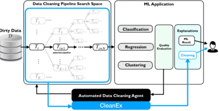
Regression Clustering State s Classification Quality Evaluation … Ti T1 … TK … Ti+1 … TK−1 … T1 Ti+1 … TK−2 … T1 Ti+1 … TK−2 … T1 Ti+1 … TK−3 … T1 Ti+N … … … … … … … … … …
Automated Data Cleaning Agent
CleanEx Explanations Cleaning ML Result selected pipeline Dirty Data D
Figure 1: CLeanEx Overview
Krishnan et al., 2015]. While important, however, we ar-gue that a critical missing piece of this line of work be the explainability of automated cleaning methods, i.e., why/how a particular data value is detected as an anomaly, how it is fixed, and why it is fixed the way it is fixed.
Current automated cleaning methods hardly ever explain their choice in building automatically data cleaning pipelines. However, the lack of convincing explanations may severely limit the scope of an end-to-end ML pipeline (including data cleaning and data preparation) and the broader adoption of ML-based Artificial Intelligence for critical decision-making. In this paper, therefore, we study the explainability of au-tomated data cleaning pipelines and propose CLeanEX, a solution that can generate explanations for a pipeline gen-erated by an automated data cleaning system that can pro-vide its pipeline search space. CLeanEX extends the auto-mated cleaning system Learn2Clean1we proposed in
[Berti-Equille, 2019a; Berti- ´Equille, 2019b], based on Q-Learning, a model-free reinforcement learning technique adapted for automating data cleaning and data preparation.
The paper proceeds as follows. In Section 2, we discuss related work. Section 3 presents our definitions and describe how to generate explanations from a sequence of cleaning tasks. Experiments are reported in Section 4. Section 5 con-cludes the paper.
1
2
Related Work
As illustrated in Fig. 1, data cleaning and preparation re-quire a sophisticated sequence of tasks Ti for the detection
and elimination of a variety of intricate data quality prob-lems (e.g., duplicates, inconsistent, missing, and outlying values). Generally, the users may not know which prepro-cessing methods can be applied to optimize the final results downstream. The selection of the optimal sequence of tasks would require for him/her executing all possible methods for each potentially relevant preprocessing task, as well as all the possible combinations of the methods with different order-ings and configurations (see all the alternative pipelines rep-resented in grey in the figure). Successfully automating this daunting manual process would definitively improve data sci-entists’ every day life. Related to our work, we review recent advances for scalable and automated data cleaning and ex-plainable systems.
ML-based data and pipeline curation. A recent line of work is to use machine learning to improve the efficiency and reliability of data cleaning and data repairing [Yakout et al., 2013; Rekatsinas et al., 2017; Krishnan et al., 2017; Shang et al., 2019]. [Yakout et al., 2013] train ML mod-els and evaluate the likelihood of recommended replacement values to fix erroneous and missing ones. [Rekatsinas et al., 2017] propose a framework for data repairing based on prob-abilistic inference to handle integrity constraints or external data sources seamlessly, with quantitative and statistical data repairing methods. [Krishnan et al., 2017] propose a method for data cleaning optimization for user-defined ML-based an-alytics. Their approach selects an ensemble of methods (sta-tistical and logic rules) and boosting to combine error detec-tion and repair. AutoML approaches can optimize the hyper-parameters of a considered ML model, but they support only a limited number of preprocessing steps with by-default meth-ods. Recently, Alpine Meadow [Shang et al., 2019] com-bines an AutoML approach and a cost model to select can-didate logical ML pipeline plans (as in DB query optimiza-tion). Multi-armed bandits are used to select promising logi-cal ML pipeline plans, and Bayesian Optimization is used to fine-tune the hyper-parameters of the selected models in the search space. However, these approaches do not provide ex-planations justifying how the data preparation pipeline search space is built and pruned. We argue that more efforts should be devoted to proposing a principled and efficient explainable automated data cleaning approach to help the user in under-standing the sequence of data preparation tasks selected by the automated cleaning system.
Explainable systems for data quality and data pro-filing. The explanation of predictive models has been an overgrowing field in the last years [Guidotti et al., 2018; Pedreschi et al., 2019]. Despite the numerous works on black box models explanation, few of them address the prob-lem of explaining the choices performed during data clean-ing tasks [Bertossi and Geerts, 2020]. [Rammelaere and Geerts, 2018] proposes to explain repairs performed by the user over small data sets by extracting the most relevant con-ditional functional dependencies (CFDs) according to the re-pairs. However, while this approach can be adapted to explain
the output of an automated data cleaning task, the CFDs can be hard to understand for the user and they have a limited expressiveness, which might be detrimental to explain the result of non rule-based repairing tasks. The T-REx frame-work [Deutch et al., 2020] provides explanations taking the form of a ranking of the set of Denial Constraints (DCs) ac-cording to their influence during the repairing process. This approach has to provide the same set of DCs that is used as input of the data repairing task. In the context of Entity Reso-lution (ER) [Ebaid et al., 2019], local explanations have been proposed to explain why a tuple pair was predicted to be a duplicate. In this context, other approaches include identify-ing a ranked list of features that contribute to the prediction as a duplicate (such as LIME [Ribeiro et al., 2016]) or as a rule that holds in the vicinity of the tuple-pair with high pre-cision (such as Anchor [Ribeiro et al., 2018]). While the cur-rent approaches explain the effect of a single repairing task, we choose to address the problem of explaining the full quence of cleaning tasks (the cleaning pipeline). As this se-quence has been selected and generated by an automated data cleaning system, we argue that the explanations should also offer the perspective related to the other candidate pipelines that were not selected by the system using various indicators to characterize the quality of an explanation.
3
Our Definitions
In this work, we represent the pipeline exploration space of the automated cleaning agent A as a tree. Each cleaning task updates the input data set and the updated version is repre-sented as a node in a tree structure: the cleaning tree. As il-lustrated in Fig. 1, the cleaning tree is composed of branches representing alternative cleaning pipelines among which the cleaning agent A may select the optimal one with respect to an ML goal and a quality performance metric. Each pipeline has features that can be used and exposed to explain the agent decision independently of the ML quality performance met-ric optimization. Explanation rules can be generated using such features. More formally, we define the cleaning tree as follows.
Definition 1 (Cleaning tree). Let D be a data set, T = {t1, . . . , tn} be the set of data preprocessing tasks that
can be executed by the automated cleaning agentA using an ML modelM that maximizes the model quality performance metricq. A cleaning tree for A, M , and q over D is an ori-ented treeCA,M,q = (V, vr, E ) such that:
• V is the set nodes formed by triples vp =
(Dp, q(M, Dp), sp) with:
– Dp, a data set resulting from the application of a
clean-ing task tp to the parent node data set or, for the root
node, the input data setD;
– q(M, Dp), the value of the quality metric of the ML
modelM measured over the pre-processed data set Dp;
– sp a vector associating, for each explanatory feature
f ∈ F , its value sp[f ] for the current node;
• vr the root node of the cleaning tree CA,M,q such that
vr∈ V and vr= (D, q(M, D), sr);
• E is the set of edges in CA,M,q, with each edgee from a
(D0, q(M, D0), s0) being labelled with the task used to clean and update D as D0. We define the bijection φ : E → V × V which maps each edge e ∈ E to the pair of nodes(v, v0) connected by e.
Definition 2 (Cleaning pipeline). Given a cleaning tree
CA,M,q = (V, v0, E ) and a node vn ∈ V. A cleaning
pipeline pvn over CA,M,q is a path σE = he1, . . . , eni of
edges inE such that there exists a sequence of nodes from V, σV = hv0, v1, . . . , vn−1, vni such that each edges ei∈ σE
connects the node vi−1 to the nodevi ∈ σV: ∀ei ∈ σE,
φ(ei) = (vi−1, vi).
After the automated cleaning agent A selects the node with the best quality metric value, the path from the root to this selected node corresponds to the best pipeline popt(M,q)that
is the optimal sequence of tasks evaluated by A for the ML model M and quality metric q.
To ground our explanations, we use explanatory features: the values of the explanatory features changing from one node to the next in a cleaning pipeline will serve as key el-ements for generating explanations of an automatically se-lected cleaning strategy. For each pipeline, we compute the following explanatory features, denoted sp[f ] in Definition 1:
• cost: The normalized cost of the pipeline;
• data quality improvement: The percentage of data quality problems solved by the pipeline (e.g., remove 100% of missing values by imputation). Note that quantifi-able data quality indicators have to be defined beforehand to characterize the main dimensions of data quality (i.e., consistency, accuracy, etc. Please see [Comignani et al., 2020; Berti- ´Equille, 2007] for more detail to specify and compute data quality indicators);
• distortion: The distortion as defined in [Dasu and Loh, 2012] as the Mahalanobis distance between the origi-nal and cleaned version of the data set;
• satisfaction: The satisfaction of ML model require-ments by the pipeline defined as a Boolean: e.g., for regres-sion, satisfaction equals 1 if linearity, multivariate normal-ity, no or little multicollinearnormal-ity, no auto-correlation, and homoscedasticity constraints are satisfied by the cleaned data set;
• corr ratio: The fraction of the number of pipelines sharing the same tasks over the sum of their respective ranks and the total number of explored pipelines; and • non corr ratio: The fraction of the number of
pipelines that do not share the same task over the sum of their respective ranks and the total number of explored pipelines.
Other features could be added but the ones we consider define a representative and relevant signature that can be used for generating meaningful explanations of a cleaning pipeline in-dependently from the ML model and the model quality metric used by the automated cleaning system.
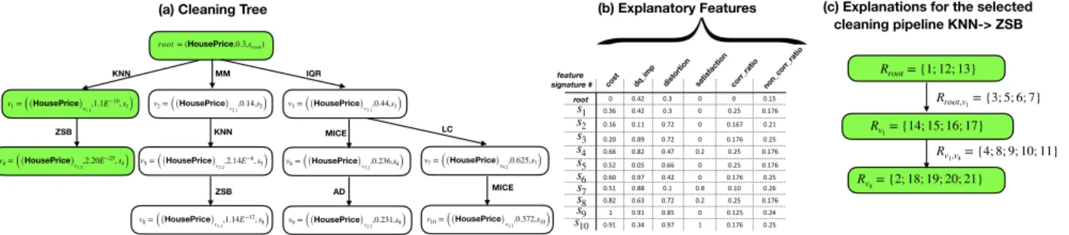
Example 1. We illustrate the notations with an example us-ing the House Price data set from Kaggle2 with 81 vari-ables and 1.46k observations to predict the SalePrice at-tribute with regression and MSE as the quality metric. We
2
https://www.kaggle.com/datasets
Table 1: Learn2Clean results on House Price data set for OLS regression over SalePrice attribute.
Rank# Sequence of Actions for Data Preparation MSE Time (ms)
1 KN N → ZSB 2.20E-25 45.1
2 M M → KN N → ZSB 1.44E-12 64.2
3 IQR → M ICE → AD 0.231 154.9
4 IQR → M ICE 0.236 94.1
5 IQR → LC → M ICE 0.372 141.5
ranLearn2Clean [Berti-Equille, 2019a] as the automated cleaning agent and reported the top-5 cleaning strategies pre-sented in Table 1 generated byLearn2Clean for OLS regres-sion. The best strategy has been selected based on minimal MSE. The MSE value, execution time (in milliseconds), and tasks of the explored cleaning pipelines are reported in the table. Data cleaning strategies include various tasks such as K-nearest neighbors (KNN) or MICE imputation, outlier detection/removal using InterQuartile Range (IQR), Z-scobased (ZSB), or LOF methods, approximate duplicate re-moval (AD), MinMax normalization (MM), and linearly cor-related (LC) feature exclusion (see [Berti-Equille, 2019a] for more details about the preprocessing methods). These strate-gies can be represented as the cleaning tree of Fig. 2(a) for which each nodevihas explanatory feature signaturesi
pre-sented in the table of Fig. 2(b). In the table, we observe cost= 0 for the root and cost= 1 for s9 as the
maxi-mal cost for the leaf node of the pipelineIQR → M ICE → AD. The pipeline KN N → ZSB selected byLearn2Clean is represented in green. corr ratio of KN N in s1 is
2
5+1+2 = 0.25 as it appears in 2 pipelines out of 5 with rank#
1 and 2 respectively (similarly forZSB). no corr ratio ofKN N is 3
5+3+4+5 = 0.176 as it does not appear in 3
pipelines ranked #3, 4, and 5 respectively.
3.1
Explaining via Feature Changes and
Comparisons
Next, we define two types of explanation predicates: (1) Change predicates that characterize the evolution of the explanatory features, and (2) Comparison predicates that characterize the relative changes by comparing with other pipelines in the cleaning tree.
Change Predicates. Given a cleaning tree
CA,M,q = (V, vr, E ), a set of features F , two distinct
nodes v, v0 ∈ V and s, s0their respective vectors of features values. We define the following set of change predicates: • succ(v, v0) iff there exists an oriented path from v to v0;
• increase(f, v, v0) iff: s[f ] < s0[f ] ∧ succ(v, v0)
• decrease(f, v, v0) iff: s[f ] > s0[f ] ∧ succ(v, v0) • stable([f0, . . . , fn], v, v0) iff:
∀fi ∈ [f0, . . . , fn], s[fi] = s0[fi] ∧ succ(v, v0)
• equiv(v, v0) iff: ∀f ∈ F , s[f ] = s0[f ].
Comparison Predicates. We define the following set of comparison predicates to express that a value of feature f for node v is respectively: (i) more, less than, or as a% of the fea-ture f values of the other nodes in the cleaning tree with a, a decimal constant in [0,1]; (ii) the best value, the worst value, or (iii) different from another node v0 feature value within a certain distance d in [0,1]:
root= (HousePrice,0.3,sroot) v1= ((HousePrice)v1.1,1.1E −10, s1) v4= ((HousePrice)v1.2,2.20E −25, s4) v2= ((HousePrice)v2.1,0.14,s2) v3= ((HousePrice)v3.1,0.44,s3) KNN ZSB MM KNN v8= ((HousePrice)v1.3,1.14E −12, s 8) ZSB v5= ((HousePrice)v2.2,2.14E −6, s5) IQR MICE v9= ((HousePrice)v2.3,0.231,s9) AD v6= ((HousePrice)v3.2,0.236,s6) LC v10= ((HousePrice)v3.3,0.372,s10) MICE v7= ((HousePrice)v4.2,0.625,s7) 0 0.42 0.3 0 0 0.15 0.36 0.42 0.3 0 0.25 0.176 0.16 0.11 0.72 0 0.167 0.21 0.20 0.89 0.72 0 0.176 0.25 0.66 0.82 0.47 0.2 0.25 0.176 0.52 0.05 0.66 0 0.25 0.176 0.60 0.97 0.42 0 0.176 0.25 0.51 0.88 0.1 0.8 0.10 0.26 0.82 0.63 0.72 0.2 0.25 0.176 1 0.91 0.85 0 0.125 0.24 0.91 0.34 0.97 1 0.176 0.25
cost dq_imp distortion satisfactioncorr_ratio non_corr_ratio
s1 s2 s3 s4 s5 s6 s7 s8 s9 s10 (b) Explanatory Features (a) Cleaning Tree
root
PS: su cc(root, v1) ∧ su cc(v1,v4): equ iv(root, v1)
C: δ(cost, root, v4,0.43) ∧ decrease(cost, root, v4)
C: δ(dq_imp, root, v4,0.4) ∧ increase(dq_imp, root, v4)
C: δ(distortion, root, v4,0.17) ∧ increase(distortion, root, v4)
C: δ(satisfaction, root, v4,1) ∧ increase(satisfaction, root, v4)
C: δ(corr_ratio, root, v4,0.55) ∧ decrease(corr_ratio, root, v4)
C: δ(non_corr_ratio, root, v4,0.05) ∧ increase(non_corr_ratio, root, v4)
C: δ(cost, v1,v4,0.43) ∧ decrease(cost, v1,v4) C: δ(dq_imp, v1,v4,0.4) ∧ increase(dq_imp, v1,v4) C: δ(distortion, v1,v4,0.17) ∧ increase(distortion, v1,v4) C: δ(satisfaction, v1,v4,1) ∧ increase(satisfaction, v1,v4) C: δ(corr_ratio, v1,v4,0.55) ∧ decrease(corr_ratio, v1,v4) C: δ(non_corr_ratio, v1,v4,0.05) ∧ increase(non_corr_ratio, v1,v4)
(c) Explanations for the selected cleaning pipeline KNN-> ZSB Rroot= {1; 12; 13} Rv4= {2; 18; 19; 20; 21} Rv1= {14; 15; 16; 17} Rroot,v1= {3; 5; 6; 7} Rv1,v4= {4; 8; 9; 10; 11} feature signature #
Figure 2: Example of a selected cleaning tree (in green) in the pipeline space of our illustrative example (a), with its corre-sponding explanatory features (b), and explanation tree (c) composed of the sets of rule IDs described in Table 2.
• more([f0, . . . , fn], v, a) iff: ∀fi∈ [f0, . . . , fn], a = |{v 0∈V|s[f i]>s0[fi]}| |V|−1 • less([f0, . . . , fn], v, a) iff: ∀fi∈ [f0, . . . , fn], a = |{v 0∈V|s[f i]<s0[fi]}| |V|−1 • as([f0, . . . , fn], v, a) iff: ∀fi∈ [f0, . . . , fn], a = |{v 0∈V|s[f i]=s0[fi]}| |V|−1 • most([f0, . . . , fn], v) iff: ∀fi∈ [f0, . . . , fn], ∀v0∈ V s.t. v 6= v0, s[fi] > s0[fi] • least([f0, . . . , fn], v) iff: ∀fi∈ [f0, . . . , fn], ∀v0∈ V s.t. v 6= v0, s[fi] < s0[fi] • δ(f, v, v0, a) iff: |s0[f ] − s[f ]| = d
Additionally to the axioms of the predicate logic, we define the following set of axioms for our explanation language: • ∀p1, p2∈ {more, as, less} s.t. p16= p2:
p1(f, v, 1) ≡ p1(f, v, 1) ∧ p2(f, v, 0) • more(f, v, a) ∧ less(f, v, a0) ≡ more(f, v, a) ∧ as(f, v, 1 − (a + a0)) ≡ as(f, v, 1 − (a + a0)) ∧ less(f, v, a0) • most([f0, . . . , fn], v) ≡ V i∈[0,n] more(fi, v, 1) • least([f0, . . . , fn], v) ≡ V i∈[0,n] less(fi, v, 1) • equiv(v1, v2) ⇔Vf ∈Fstable(f, v1, v2)
Now, we can define formally the explanation rules that will be automatically generated.
Definition 3 (Explanation Rule). Given a cleaning tree
CA,M,q = (V, vr, E ), a feature f in F , v and v0 two nodes
inV, three decimals constants, a, a0, a00∈ [0, 1], and the
ex-planation predicates:
p0∈ {increase; stable; decrease};
p1, p2∈ {more; as; less} such that p16= p2;
p3∈ {most; least}.
We define the following types of explanation rules:
Pv,v0 : ∃v1, . . . , vn ∈ V, succ(v, v1) ∧ . . . ∧ succ(vn, v0) Bf,v,v0 : p0(f, v, v0) ∧ δ(f, v, v0, a) Cf,v: p1(f, v, a0) ∧ p2(f, v, a00) Ef,v: p3(f, v) Sf,v,v0 : stable(f, v, v0) Sv,v0 : equiv(v, v0)
Table 2: Explanation rules generated for pipeline#1 KN N → ZSB
Rule# Type Rule
0 P succ(root, n1) ∧ succ(n1, n4)
1 E least([cost, corr ratio, non corr ratio], root)
2 E most([cost, dq imp, distortion, satisfaction], n4)
3 S stable([dq imp, distortion, satisfaction], root, n1)
4 S stable([corr ratio, non corr ratio], n1, n4)
5 B increase(cost, root, v1) ∧ δ(cost, root, v1, 0.36)
6 B increase(corr ratio, root, v1) ∧ δ(corr ratio, root, v1, 0.25)
7 B increase(non corr ratio, root, v1)
∧δ(non corr ratio, root, v1, 0.026)
8 B increase(cost,v1, v4) ∧ δ(cost, v1, v4, 0.3)
9 B increase(dq imp, v1, v4) ∧ δ(dq imp, v1, v4, 0.4)
10 B increase(distortion, v1, v4) ∧ δ(distortion, v1, v4, 0.17)
11 B increase(satisfaction, v1, v4) ∧ δ(satisfaction, v1, v4, 0.2)
12 C as([dq imp, distortion, satisfaction], root, 0.5)
13 less([dq imp, distortion, satisfaction], root, 0.5)
14 C less(cost, v1, 0.5)
15 C more(cost, v1, 0.5)
16 C as([dq imp, distortion, satisfaction, corr ratio,
non corr ratio], v1, 0.5)
17 C less([dq imp, distortion, satisfaction, corr ratio,
non corr ratio], v1, 0.5)
18 C as(corr ratio, v4, 0.5)
19 C more(corr ratio, v4, 0.5)
20 C as(non corr ratio, v4, 0.5)
21 C more(non corr ratio, v4, 0.5)
TypeP explanation rules are path explanations between two nodesv and v0. Type B explanation rules are behavior change
explanations witha constant representing the δ change value of some featuref between two nodes v and v0. Type C ex-planations are comparative exex-planations with respect to the change of other nodes. Type E explanation rules are related to extreme value description. Type S explanation rules are stability explanation rules betweenv and v0.
These explanation rules can be either focused on one fea-ture f for the Sf,v,v0explanation rules, or all the features
cov-ered by CA,M,q for the Sv,v0 explanation rules. Table 2 gives
the explanation rules automatically generated for the cleaning pipeline KN N → ZSB. Finally, all the generated rules can be organized into an explanation tree mirroring the cleaning tree defined earlier, as follows.
Definition 4 (Explanation Tree). Let CA,M,q = (V, vr, E )
be a cleaning tree andR be a set of explanation rules such
thatCA,M,q |= R. An explanation tree for R in CA,M,q is an
oriented treeXC = (V, E ) such that:
• V is the set nodes such that each node vRiis formed by the
subset of rulesRi ⊆ R such that each r ∈ Riis a rule of
typeCf,viorEf,vi;
• E is the set of edges in XC, with each edgee from a node
rulesRi,jsuch that eachr ∈ Ri,jis a rule of typeBf,vi,vj,
Sf,vi,vj orSvi,vj.
The branch of the explanation tree corresponding to the selected pipeline of the example is provided in Fig. 2(c).
3.2
Quality Indicators of Explanations
Given an explanation tree XC, its set of predicates,
denoted PC including the set of predicates Pml of
the form most([f0, . . . , fn], v) or least([f0, . . . , fn], v),
f eatures(p), the function returning the set of features cov-ered by a predicate p, and delta(r) the function returning the value a of the delta predicate δ(f, v, v0, a) in a rule r. We select the best explanations to provide to the user using the following relevant quality indicators defined as follows. Definition 5 (Polarity). The polarity of XCis defined as:
polarity(XC) = P ∀p∈Pml|f eatures(p)| P ∀p0∈PC|f eatures(p0)| .
Definition 6 (Distancing). Given the set X of explanation trees overCA,M,q such thatXC 6∈ X. The distancing of XC is
defined as:
distancing(XC) =
P
∀ delta predicate r in XCdelta(r)
P
∀ delta predicate r in Xdelta(r)
.
Definition 7 (Surprise). Given a set X of explanation trees
overCA,M,qsuch thatXC 6∈ X. The surprise of XC is defined
as:
surprise(XC) =
P
∀X ∈X
P
∀ rule r of type B in Xdelta(r)
P
∀predicate p in Xf eatures(p)
.
Definition 8 (Diversity). Given S the set of all predicates symbols excepting δ in the rules of XC (defined in Def. 3
for P,B,C,E and S types of explanations), and Ps the set of
all predicates with predicate symbols in the rules of XC.The
diversity ofXC is defined as:
diversity(XC) = − P ∀s∈S ns N log2 ns N |S|
withns, the number of nodes features over predicates with
symbols: ns= P
∀p∈Ps
|f eatures(p)|, and N , the total num-ber of nodes features:N = P
∀s∈S
P
∀p∈Ps
|f eatures(p)|.
3.3
Multi-Objective Optimization
Next, we use these quality indicators as optimization objec-tives to select the optimal explanations of the automated choice of a cleaning pipeline. When dealing with more than one dimension to optimize, there may be many incomparable sets of explanation. Therefore, we adapt the notion of expla-nation plan and Pareto plan as follows.
Definition 9 (Explanation Plan). Explana-tion plan πi, associated to xi, a branch of
an explanation tree XC, is a tuple πi =
hpolarity(xi), distancing(xi), surprise(xi), diversity(xi)i.
Definition 10 (Explanation Sub-Plan). Explanation plan πi
is the sub-plan of another planπj if their associated
expla-nation sub-trees satisfyxi⊆ xj.
Algorithm 1 Approximated Pareto-optimal Explanations Input: The user-defined optimization objective O, the
preci-sion value α, the maximum number of rules of an ex-planation k, the exex-planation tree X , and the pipeline to explain x
Output: The set of explanations Παfor x
1 Πα←− πx
2 for all explanation branches B of the tree X \ x do 3 πB←− construct plan(B)
4 if πBis notα-dominated wrt O by any other plan in Πα 5 then Πα.add(πB)
6 for d ∈ [1, k] do
7 for all explanation branches b of d rules in X \ x do 8 πb←− construct plan(b)
9 if πbis notα-dominated wrt O by any other plan in Πα 10 then Πα.add(πb)
11 return Πα
Definition 11 (Dominance). Plan π1dominatesπ2ifπ1has
better or equivalent values thanπ2 in every quality
indica-tor. The term better is equivalent to greater for maximization objectives (e.g., diversity or polarity), and lower form in min-imization ones (e.g., distancing or surprise) depending on the user’s preferences. Furthermore, planπ1strictly dominates
π2ifπ1dominatesπ2and the values of indicators forπ1and
π2are not equal.
Definition 12 (Pareto Plan). Plan πi is Pareto if no other
plan strictly dominatesπi. The set of all Pareto plans is
de-noted asΠ.
Now, we define our problem as a multi-objective optimiza-tion (MOO) problem as follows: for an explanaoptimiza-tion tree XC,
the problem is to find all the explanation branches x, such that each branch satisfies:
• diversity(x) is maximized; • surprise(x) is optimized; • polarity(x) is optimized; • distancing(x) is optimized;
Note that while we always maximize diversity, we may ei-ther minimize or maximize the distancing, surprise, and po-larity based on the user’s needs. The main challenge in de-signing an algorithm for finding optimal explanations of auto-mated data cleaning is the multi-objective nature of the prob-lem. A multi-objective problem can be easily solved if it is possible to combine all quality indicators into one or if the op-timization of one indicator leads an optimized value of other indicators. However, in our problem, the indicators may be conflicting, i.e., optimizing one does not necessarily lead to an optimized value for others and they cannot be combined into one single indicator. Therefore, we propose Algorithm 1 based on approximation to select the Pareto-optimal explana-tion rules. The algorithm makes less enumeraexplana-tions with a the-oretical guarantee on the quality of results. Its pruning mech-anism uses the precision value α. In the special case of α = 1, the algorithm operates exhaustively. If α > 1, the algorithm prunes more and hence is faster. In the latter case, a new plan is only compared with all plans that generate the same result. But a new plan are only inserted into the buffer if no other
C58 : increase(cost, root, n7) ∧ δ(cost, root, n7,0.332) C70 : least([satisfaction], n7)
C59 : d ecrease(d q_imp, root, n7) ∧ δ(d q_imp, root, n7,0.332) C72 : less([cost], n7,0.1)
C71 : more([cost], n7,0.9)
Maximize diversity Maximize surprise
C85 : most([d q_imp, corr_ratio], root) C115 : more([cost], root,0.3) C105 : less([cost], root,0.7) C125 : less([d istortion], root,0.8) Minimize all indicators
C34 : increase(cost, root, n7) ∧ δ(cost, root, n7,0.332) C35 : d ecrease(d q_imp, root, n7) ∧ δ(d q_imp, root, n7,0.332) C36 : increase(d istortion, root, n7) ∧ δ(d istortion, root, n7,0.091) C37 : d ecrease(satisfaction, root, n7) ∧ δ(satisfaction, root, n7,0.005)
Maximize all indicators Maximize polarity
C58 : increase(cost, root, n7) ∧ δ(cost, root, n7,0.332) C71 : most([corr_ratio, d q_imp], root) C81 : least([non_corr_ratio], root) C160 : least([satisfaction], n7)
Maximize distancing
C28 : increase(cost, root, n7) ∧ δ(cost, root, n7,0.332) C29 : d ecrease(d q_imp, root, n7) ∧ δ(d q_imp, root, n7,0.332) C30 : increase(d istortion, root, n7) ∧ δ(d istortion, root, n7,0.091) C32 : d ecrease(corr_ratio, root, n7) ∧ δ(corr_ratio, root, n7,0.892) C33 : increase(non_corr_ratio, root, n7) ∧ δ(non_corr_ratio, root, n7,0.686) C26 : d ecrease(corr_ratio, root, n7) ∧ δ(corr_ratio, root, n7,0.892)
C27 : increase(non_corr_ratio, root, n7) C107 : least([satisfaction], n7) C145 : most([d q_imp, corr_ratio], root) C155 : least([non_corr_ratio], root) ∧ δ(non_corr_ratio, root, n7,0.686) Max_all Max_Polarity Max_distancing Max_diversity Max_surprise Objectives Number of Rules Ex pla nation R anki ng max_de pt h
Figure 3. Optimal sets of explanations with their quality indicators
depending on the multiple (left) single (right) objectives Figure 4. Explanation ranking with varying explanation tree depth, objectives, and number of rules
1 10 100 1000 10000 100000 1 2 3 4 5 1 2 3 4 5 1 2 3 4 5 1 2 3 4 5 1 2 3 4 5 1 2 3 4 5 1 2 3 4 5 1 2 3 4 5 (-;-;-;-) (+;-;-;-) (+;-;+;-) (+;+;+;+) (+;0;0;0) (0;+;0;0) (0;0;+;0) (0;0;0;+) Av er ag e Ti m e (s ) Execution time with varying cleaning tree size and optimization objectives size=10 size=100 diversity diversity diversityE3 surprise surprise surprise
Figure 3. Quality Indicators
Figure 5. Time with varying explanation tree size (10, 100), max_depth (1 to 5), and objectives
diversity E2 E1 E4 E3 E2 E1 E3 E2 E1 E4 E3 E2 E1
E4 Min_all Max_polarity_ Max_all Max_polarity Max_distancing Max_surprise Max_diversity
Min_others Max_polarity_surprise
_Min_others
plan approximately dominates it. This means that the algo-rithm ends to insert fewer plans than the exhaustive variant. Given a maximization objective O (e.g., diversity, surprise, distancing, polarity), plan π1with sub-plans π11and π12, and
α. Derive π2 from π1 by replacing π11 by π21and π12 by
π22. Then O(x21) ≥ O(x11) × α and O(x22) ≥ O(x12) × α
together imply O(x2) ≥ O(x1) × α. Similarly, the extension
for a minimization objective is straightforward.
The algorithm 1 exploits a dynamic programming ap-proach. The algorithm begins by constructing a plan for each single branch of an explanation tree (lines 2 to 3). It keeps all non α-dominated plans in a buffer. Then, it examines all the branches of the explanation tree with depth 1 up to k (lines 6 to 10). After each iteration, it removes α-dominated plans from the buffer. Finally, it returns the buffer content as result.
4
Preliminary Experiments
Based on our observations from the automated cleaning pipeline search spaces, we generated two types of clean-ing tree structures with 10 and 100 nodes respectively and a maximal depth varying from 1 to 5 levels from root to leaves. The number of nodes per level follows a Beta dis-tribution (alpha=2, beta=2.35). The values of the six ex-planatory features were generated randomly five times. We ran five trials of picking one cleaning pipeline to explain among all the candidate ones for each of the 250 configu-rations (2 × 5 × 5 × 5) and we averaged the results. We perform all experiments on a laptop Dell XPS machine with an Intel Core i7-7500U quad-core, 2.8 GHz, 16 GB RAM, powered by Windows 10 64-bit with Python. CLeanEX, data sets, and more detailed experiments are available at
https://github.com/ucomignani/cleanex.
Fig. 3 illustrates different Type C explanations for explain-ing the same cleanexplain-ing pipeline. Each set of explanations has
been selected as it optimizes specific objectives in terms of quality indicators. We can observe that in general, no correla-tion exists between the optimized value of the objectives and the explanation set can be very different. Thus, each objec-tive should be optimized independently and according to the user’s preferences. Fig. 4 shows the result of our algorithm (with α = 1 exhaustive search) for the top-10 ranked explana-tions depending on the optimization objectives. The ranking depends on the explanation size and the maximal depth of the tree: 2-3 rules for the explanations maximizing all objectives for depth from 2-3 (Max all). In Fig. 5, we can also exam-ine the effect of the tree structure (in terms of the number of nodes and maximal depth) on execution time of CLeanEX to find the optimal explanations. We observe that the execu-tion times for trees containing 10 and 100 nodes have similar values as their respective depth increases. The reason is that the number of subsets of candidate rules for a given branch increases quickly when the depth of the tree also increases. Inversely, reducing the depth of the branches increases the number of branches to explore, for which the depth generally decreases, reducing the time complexity for the cases with few nodes. The execution time of our algorithm is spent on the computation of the quality indicators, the generation of the rules, and the exploration of a large number of candidates rules sets. However, changing α will reduced this last dimen-sion while providing an approximation guarantee.
5
Conclusions
In this paper, we propose CLeanEX, a framework to gener-ate explanations for automgener-ated data cleaning. The key ad-vantages of our approach is that our explanation system is: (1) model-agnostic: it can be applied to any ML model, any set of data cleaning tasks, and any automated cleaning agent that can provide its cleaning pipeline search space; (2) logic-based: explanations are comprehensible to humans with di-verse expertise and can be extensible to handle causal reason-ing; (3) both local and global: it can explain both some part or the whole cleaning pipeline; (4) model quality-independent: it provides a reliable set of explanations independently from the ML model quality performance metric that is used by the automated cleaning agent for the selection of the optimal cleaning pipeline; and (5) user-defined: optimization is based on the user’s objectives.
References
[Berti- ´Equille, 2007] Laure Berti- ´Equille. Quality Awareness for Data Management and Mining. HDR, Univ. Rennes 1, France, http://pageperso.lis-lab.fr/˜laure.berti/ pub/Habilitation-Laure-Berti-Equille.pdf, 2007.
[Berti-Equille, 2019a] L. Berti-Equille. Learn2Clean: Optimizing the Sequence of Tasks for Web Data Preparation. In Proc. of the World Wide Web Conference, The Web Conf 2019, pages 2580– 2586, 2019.
[Berti- ´Equille, 2019b] Laure Berti- ´Equille. Reinforcement learning for data preparation with active reward learning. In Proc. of the 6th International Conference on Internet Science, INSCI 2019, pages 121–132, 2019.
[Bertossi and Geerts, 2020] L. Bertossi and F. Geerts. Data quality and explainable ai. ACM Data and Information Quality J., 2020. [Comignani et al., 2020] Ugo Comignani, No¨el Novelli, and Laure
Berti- ´Equille. Data quality checking for machine learning with
mesqual. In Proc. of the 23nd International Conference on
Extending Database Technology, EDBT 2020, pages 591–594, 2020.
[Dasu and Loh, 2012] T. Dasu and J. M. Loh. Statistical distortion: Consequences of data cleaning. PVLDB, 5(11):1674–1683, 2012. [Deutch et al., 2020] D. Deutch, N. Frost, A. Gilad, and O. Schef-fer. T-rex: Table repair explanations. In ACM SIGMOD, 2020. [Ebaid et al., 2019] A. Ebaid, S. Thirumuruganathan, W. G. Aref,
A. K. Elmagarmid, and M. Ouzzani. EXPLAINER: entity reso-lution explanations. In IEEE ICDE, pages 2000–2003, 2019. [Guidotti et al., 2018] R. Guidotti, A. Monreale, S. Ruggieri,
F. Turini, F. Giannotti, and D. Pedreschi. A survey of methods for explaining black box models. ACM Comput. Surv., 51(5), August 2018.
[Krishnan et al., 2015] S. Krishnan, J. Wang, M. J. Franklin,
K. Goldberg, T. Kraska, T. Milo, and E. Wu. Sampleclean:
Fast and reliable analytics on dirty data. IEEE Data Eng. Bull., 38(3):59–75, 2015.
[Krishnan et al., 2017] S. Krishnan, M. J. Franklin, K. Goldberg, and E. Wu. Boostclean: Automated error detection and repair for machine learning. CoRR, abs/1711.01299, 2017.
[Pedreschi et al., 2019] D. Pedreschi, F. Giannotti, R. Guidotti, A. Monreale, S. Ruggieri, and F. Turini. Meaningful explana-tions of black box ai decision systems. In AAAI, volume 33, pages 9780–9784, 2019.
[Rammelaere and Geerts, 2018] J. Rammelaere and F. Geerts. Ex-plaining repaired data with cfds. PVLDB, 11(11):1387–1399, 2018.
[Rekatsinas et al., 2017] T. Rekatsinas, X. Chu, I. F. Ilyas, and C. R´e. Holoclean: Holistic data repairs with probabilistic in-ference. PVLDB, 10(11):1190–1201, 2017.
[Ribeiro et al., 2016] M. T. Ribeiro, S. Singh, and C. Guestrin. ”why should I trust you?”: Explaining the predictions of any clas-sifier. In ACM SIGKDD 2016, pages 1135–1144, 2016.
[Ribeiro et al., 2018] M. T. Ribeiro, S. Singh, and C. Guestrin. An-chors: High-precision model-agnostic explanations. In AAAI, 2018.
[Shang et al., 2019] Z. Shang, E. Zgraggen, B. Buratti, F. Koss-mann, P. EichKoss-mann, Y. Chung, C. Binnig, E. Upfal, and
T. Kraska. Democratizing data science through interactive cu-ration of ML pipelines. In ACM SIGMOD, pages 1171–1188, 2019.
[Yakout et al., 2013] M. Yakout, L. Berti- ´Equille, and A. K. Elma-garmid. Don’t be scared: use scalable automatic repairing with maximal likelihood and bounded changes. In ACM SIGMOD, pages 553–564, 2013.