Recoverable Robust Timetables: An Algorithmic Approach on Trees

HAL Id: hal-00643980

https://hal.inria.fr/hal-00643980

Submitted on 23 Nov 2011

HAL is a multi-disciplinary open access

archive for the deposit and dissemination of

sci-entific research documents, whether they are

pub-lished or not. The documents may come from

teaching and research institutions in France or

abroad, or from public or private research centers.

L’archive ouverte pluridisciplinaire HAL, est

destinée au dépôt et à la diffusion de documents

scientifiques de niveau recherche, publiés ou non,

émanant des établissements d’enseignement et de

recherche français ou étrangers, des laboratoires

publics ou privés.

Approach on Trees

Gianlorenzo d’Angelo, Gabriele Di Stefano, Alfredo Navarra, Cristina Pinotti

To cite this version:

Gianlorenzo d’Angelo, Gabriele Di Stefano, Alfredo Navarra, Cristina Pinotti. Recoverable Robust

Timetables: An Algorithmic Approach on Trees. IEEE Transactions on Computers, Institute of

Electrical and Electronics Engineers, 2011, 60 (3), pp.433 - 446. �10.1109/TC.2010.142�. �hal-00643980�

Recoverable Robust Timetables: an Algorithmic

Approach on Trees

Gianlorenzo D’Angelo, Gabriele Di Stefano, Alfredo Navarra, and Cristina M. Pinotti

Abstract—In the context of scheduling and timetabling, we study a challenging combinatorial problem which is very interesting for both practical and theoretical points of view. The motivation behind it is to cope with scheduled activities which might be subject to unavoidable disruptions, such as delays, occurring during the operational phase. The idea is to preventively plan some extra time for the scheduled activities in order to be “prepared” if a delay occurs, and absorb it without the necessity of re-scheduling all the activities from scratch. This realizes the concept of designing robust timetables. During the planning phase, one should also consider recovery features that might be applied at runtime if disruptions occur. This leads to the concept of recoverable robust timetables. In this new concept, it is assumed that recovery capabilities are given as input along with the possible disruptions that must be considered. The main objective is the minimization of the overall needed time. The quality of a robust timetable is measured by the price of robustness, i.e. the ratio between the cost of the robust timetable and that of a non-robust optimal timetable. We show that finding an optimal solution for this problem isN P-hard even though the topology of the network, which models dependencies among activities, is restricted to trees. However, we manage to design a pseudo-polynomial time algorithm based on dynamic programming and apply it on both random networks and real case scenarios provided by Italian railways. We evaluate the effect of robustness on the scheduling of the activities and provide the price of robustness with respect to different scenarios. We experimentally show the practical effectiveness and efficiency of the proposed algorithm.

✦

Index Terms—Timetable, Scheduling Activities, Robustness, Price of

Ribusteness, Combinatorial Optimization, Dynamic Programming

1

I

In many real-world applications, the design of a solution is divided in two main phases: a strategic planning phase and an operational planning phase. The two planning phases differ in the time in which they are applied. The strategic planning phase aims to plan how to optimize the use of the available resources according to some objective function before the system starts operating. The operational planning phase aims to have immediate reaction to disturbing events that can occur when the system is running. In general, the objectives of strategic and operational planning might be in conflict with each other. As disturbing events are unavoidable in large and complex systems, it is fundamental to understand the interaction between the objectives of the two phases. An example of real-world systems, where this interaction is important, is the timetable planning in railway systems. It arises in the strategic planning phase and requires to compute a timetable for passenger trains that deter-mines minimal passenger waiting times. However, many

• G. D’Angelo and G. Di Stefano are with the Department of Electrical and Information Engineering, University of L’Aquila, L’Aquila, Italy. Email:{gianlorenzo.dangelo, gabriele.distefano}@univaq.it

• A. Navarra and C. M. Pinotti are with the Department of Mathe-matics and Computer Science, University of Perugia, Perugia, Italy. Email:{navarra, pinotti}@dmi.unipg.it

This work was partially supported by the Future and Emerging Technologies Unit of EC (IST priority - 6th FP), under contract no. FP6-021235-2 (project ARRIVAL).

Preliminary results contained in this paper appeared in [6], [7], [8].

disturbing events might occur during the operational phase, and they might completely change the scheduled activities. The main effect of the disturbing events is the arising of delays. The conflicting objectives of strategic against operational planning are evident in timetable optimization. In fact, a train schedule that lets trains sit in stations for some time will not suffer from small delays of arriving trains, because delayed passengers can still catch potential connecting trains. On the other hand, large delays can cause passengers to lose trains and hence imply extra traveling time. The problem of deciding when to guarantee connections from a delayed train to a connecting train is known as delay management (see [3], [9], [11], [12], [15], [16]). Despite its natural for-malization, the problem turns out to be very complicated to be optimally solved. In fact, it is N P -hard in the general case, while it is polynomial in some particular cases (see [3], [4], [11], [12], [15], [16]).

To cope with the management of delays, we follow the recent recoverable robustness approach provided in [2], [5] and [14], continuing the recent studying in robust optimization. Our aim is the design of timetables in the strategic planning phase in order to be “prepared” to react against possible delays. If a delay occurs, the de-signed timetable should guarantee to recover the sched-uled events by means of allowed operations represented by given recovery algorithms. Events and dependencies among events are modeled by means of an event activity network (see [3], [4], [16], [17]). This is a directed graph where the nodes represent events (e.g., arrival or de-parture of trains) and arcs represent activities occurring between events (e.g., waiting in a train, driving between stations or changing to another train). We assume that

only one delay of at most α time might occur at a generic activity of the scheduled event activity network. An activity may absorb the delay if it is associated with a so called slack time. A slack time assigned to an activity represents some extra available time that can be used to absorb limited delays. Clearly, if we associate a slack time of at least α to each activity, every delay can be locally absorbed. However, this approach is not practical as the overall duration time of the scheduled events would increase too much. We plan timetables able to absorb the possible occurring delay within a fixed amount of events, ∆. This means that, if a delay occurs, it is not required that the delay is immediately absorbed (unless ∆ = 0) but it can propagate to a limited number of activities in the network. Namely, the propagation might involve at most ∆ events. The objective function is then to minimize the total time required by the activities in order to serve all the scheduled events and to be robust with respect to one possible delay. The challeng-ing combinatorial problem arischalleng-ing by those restrictions is of its own interest. We restrict our attention to event activity networks whose topology is a tree. In fact, in [3], the authors show that the described problem is N P -hard when the event activity network topology is a directed acyclic graph, and they provide approximation algorithms which cope with the case of ∆ = 0. In [4], these algorithms have been extended to ∆ ≥ 0.

In this paper, we study event activity networks which have a tree topology. Surprisingly, the described problem turns out to be N P -hard even in this restricted case. For trees, we present an algorithm that solves the problem, when ∆ ≥ 1, in O(∆2_{n) time and O(∆n) space, where n}

is the number of events in the input event activity net-work. Whereas, O(n) time and O(n) space are required to solve the problem when ∆ = 0. The result implies that the problem can be solved in pseudo-polynomial time. In fact, the parameter ∆ can be clearly provided using dlog ∆e bits. Moreover, since we prove that the size of some input event activity network instances, for which the problem remains N P -hard, can be encoded by means of O(log n) bits, the proposed algorithm is also pseudo-polynomial in n. The algorithm exploits the tree topology in order to choose which arc must be associated with some slack time. On trees, intuitively, we prove that the choice to carefully postpone the assignment of a slack time to descendent activities as much as possible leads to cheapest solutions. Another interesting property for tree topologies when ∆ ≥ 1 shows that there is always an optimal solution without two consecutive activities both associated with a slack time. We also implement the algorithm and test its performances on both real case and random scenarios. Based on data provided by Trenitalia [18], we make use of the devised algorithm in order to obtain robust timetables with respect to the possibility of an occurring delay of duration α. We show and discuss the interesting obtained results about the applicability and the low costs in terms of slack times needed for making robust the considered timetables

with respect to different scenarios. The small execution time elapsed by the algorithm on real-world instances revels its effective applicability. Moreover, experiments on random instances show that the good behavior of the algorithm does not depend on the particular structure of the input tree arising from the real-world instances.

1.1 Outline

The next section describes the model used to transform an optimization problem into a recoverable robust prob-lem as shown in [5]. Section 3 presents the timetabling problem and its recoverable robust version. Section 4 is devoted to the study of the computational complexity required for solving the proposed recoverable robust timetabling. Section 5 presents the pseudo-polynomial time algorithm and provides its correctness. Section 6 is devoted to the experimental studies obtained by apply-ing the algorithm to real-world and random instances. Finally, Section 7 provides conclusive remarks and useful outcomes for further investigation on the studied prob-lem.

2

R

R

M

In this section, we summarize the model of recoverable robustness given in [5]. Such a model describes how an optimization problem P can be turned into a robustness problem P. Hence, concepts like robust solution, robust algorithm for P and price of robustness are defined. In the remainder, an optimization problem P is characterized by the following parameters. A set I of instances of P ; a function F that associates to any instance i ∈ I the set of all feasible solutions for i; and an objective function f : S → R where S =S_i∈IF (i) is the set of all feasible solu-tions for P . Without loss of generality, from now on we consider minimization problems. Additional concepts to introduce robustness requirements for a minimization problem P are needed:

• M : I → 2I – a modification function for instances

of P . Let i ∈ I be the considered input to the problem P . A disruption is meant as a modification to the input i. Hence, M (i) represents the set of disruptions of the input of P that can be obtained by applying all possible modifications to i.

• A – a class of recovery algorithms for P . Algorithms

in A represent the capability of recovering against disruptions. An element Arec∈ A works as follows: given (i, π) ∈ I × S, an instance/solution pair for P , and j ∈ M (i), a disruption of the current instance i, then Arec(i, π, j) = π0_{, where π}0_{∈ F (j) represents} the recovered solution for P .

Definition 2.1: A recoverable robustness problem P is de-fined by the triple (P, M, A). All the recoverable robust-ness problems form the class RRP.

Definition 2.2: Let P = (P, M, A) ∈ RRP. Given an instance i ∈ I for P , an element π ∈ F (i) is a feasible

solution for i with respect to P if and only if the following relationship holds:

∃Arec∈ A : ∀j ∈ M (i), Arec(i, π, j) ∈ F (j). In other words, π ∈ F (i) is feasible for i with respect to P if it can be recovered by applying some algorithm Arec ∈ A for each possible disruption j ∈ M (i). The solution π is called a robust solution for i with respect to problem P . The quality of a robust solution is measured by the price of robustness.

Definition 2.3: Let P = (P, M, A) ∈ RRP. A robust algorithm for P is an algorithm Arob such that, for each i ∈ I, Arob(i) is a robust solution for i with respect to P .

Definition 2.4: Let P ∈ RRP and let Arob be a robust algorithm for P. The price of robustness of Arob is:

Prob(P, Arob) = max i∈I ½ f (Arob(i)) min{f (π) : π ∈ F (i)} ¾ . The price of robustness of P is:

Prob(P) = min{Prob(P, Arob) : Arob is robust for P}. Arob is P-optimal if Prob(P, Arob) = Prob(P). A robust solution π for i ∈ I is P-optimal if

f (π) = min {f (π0_{) : π}0 _{is feasible for i w.r.t. P} .}

3

R

T

P

In this section, we turn a particular timetable problem (T T ) into a recoverable robustness problem, the Robust Timetabling problem (RTT ).

Given a Directed Acyclic Graph (DAG) G = (V, A), where the nodes represent events and the arcs represent the activities1_{, the timetabling problem consists in}

assign-ing a time to each event in such a way that all the constraints provided by the set of activities are respected. Specifically, given a function L : A → N that assigns the minimal duration time to each activity, a solution π ∈ R|V |_≥0 for the timetable problem on G is found by assigning a time π(u) to each event u ∈ V such that π(v) − π(u) ≥ L(a) for all a = (u, v) ∈ A.

Given a function w : V → R≥0 that assigns a weight to each event, an optimal solution for the timetabling problem minimizes the total weighted time for all events. Formally, the timetabling problem T T is defined as fol-lows.

T T

GIVEN: A DAG G = (V, A), functions L : A → N and

w : V → R≥0.

PROB.: Find a function π : V → R≥0 such that π(v) − π(u) ≥ L(a) for all a = (u, v) ∈ A and f (π) = P

v∈V w(v)π(v) is minimal.

Then, an instance i of T T is specified by a triple (G, L, w), where G is a DAG, L associates a minimal 1. Indeed G is the so called event activity network described in the introduction.

duration time to each activity, and w associates a weight to each event. The set of feasible solutions for i is: F (i) = {π : π(u) ∈ R≥0, ∀u ∈ V and π(v) − π(u) ≥ L(a), ∀a = (u, v) ∈ A}.

A feasible solution for T T may induce a positive slack time sπ(a) = π(v) − π(u) − L(a) for each a ∈ A. That is, the planned duration π(v) − π(u) of an activity a = (u, v) is greater than the minimal duration time L(a).

When in T T the DAG is an out-tree T = (V, A), any feasible solution satisfies, for each v ∈ V , π(v) ≥ π(r) + P

a∈P (r,v)L(a), where r is the root of T and P (r, v) the directed path from r to v in T . Moreover, without loss of generality, we can focus our attention only on instances of T T with L(a) = 1 ∀a ∈ A. Indeed, as proved below, the cost f (π) of a feasible solution π for an instance of T T with an arbitrary function L easily derives from the cost f (π0_{) of a feasible solution π}0 _{for the same instance} of T T with L0_{(a) = 1, ∀a ∈ A.}

Lemma 3.1: Consider an out-tree T = (V, A), rooted at r, and an instance i = (T, L, w) of T T . Let i0_{= (T, L}0_{, w)} be an instance such that L0_{(a) = 1, ∀a ∈ A. For any} feasible solution π for i, there exists a feasible solution π0 _{for i}0 _{such that}

f (π) = f (π0_{) +}X v∈V

X a∈P (r,v)

w(v)(L(a) − 1). Proof: Any feasible solution π of i is in the form:

π(v) = π(r) + X a∈P (r,v) (L(a) + sπ(a)), v ∈ V. We define π0 _{as π}0_{(r) = π(r) and} π0_{(v) = π}0_{(r) +} X a∈P (r,v) (1 + sπ(a)).

Note that, π0 _{is feasible for i}0_{. The values of the} objective functions of π and π0 _are

f (π) = π(r)w(r) +X v∈V π(v)w(v) = = π(r)w(r) +X v∈V X a∈P (r,v) (L(a) + sπ(a))w(v) and f (π0_{) = π}0_{(r)w(r) +}X v∈V π0_{(v)w(v) =} = π(r)w(r) +X v∈V X a∈P (r,v) (1 + sπ(a))w(v), respectively. Hence, f (π) = f (π0_{) +}X v∈V X a∈P (r,v) w(v)(L(a) − 1).

Problem T T can be solved in linear time by assigning the minimal possible time to each event (i.e. by using the Critical Path Method [13]). However, such a solu-tion cannot always cope with possible delays occurring at running time to the activities. Recovery (on-line)

strategies might be necessary. For this reason, let now transform T T into a recoverable robustness problem RTT = (T T , M, A), according to Section 2. Given an instance i = (G, L, w) for T T and a constant α ∈ N, we limit the modifications on i by admitting a single delay of at most α time. We model it as an increase on the minimal duration time of the delayed activity. Formally, M (i) is defined as follows: M (i) = {(G, L0_{, w) : ∃ ¯a ∈ A :} L(¯a) ≤ L0_{(¯a) ≤ L(¯a) + α, L}0_{(a) = L(a) ∀a 6= ¯a}.}

We define the class of recovery algorithms A for T T by introducing the concept of events affected by one delay.

Definition 3.2: Given a DAG G = (V, A), a function s : A → R≥0, and a number α ∈ R≥0, a node x is α-affected by a = (u, v) ∈ A (or a α-affects x) if there exists a path p = (u ≡ v0, v ≡ v1, . . . , vk ≡ x) in G such that Pk

i=1s((vi−1, vi)) < α. The set of nodes α-affected by an arc a = (u, v) is denoted as Aff(a).

In the following, given a feasible solution π for T T , we will use the slack times sπ defined by π as the function s in the previous definition. Thus, an event x is affected by a delay α occurring on the arc a = (u, v) if the sum of the slack times assigned by the function π to the events on the path from u to x is smaller than α. That is, the planned durations of the activities are not able to absorb the delay α and thus x will be delayed.

We assume that the recovery capabilities allow to change the time of at most ∆ events. Formally, given ∆ ∈ N, each algorithm in A is able to compute a feasible solution π0 _{if |Aff(a)| ≤ ∆ for each a ∈ A. This} implies that a robust solution for RTT must guarantee that a delay of at most α time may affect at most ∆ events. Note that, RTT only requires to find a feasible solution. Nevertheless, it is worth to find a solution that minimizes the objective function of T T .

From now on, we restrict our attention to rooted out-trees and we define the RTToptoptimization problem as follows:

RTTopt

GIVEN: A tree T = (V, A), a function w : V → R≥0, and

α, ∆ ∈ N.

PROB.: Find a function π : V → R≥0 s. t. each arc in A α-affects at most ∆ nodes, according to the function sπ : A → R≥0 defined as sπ(a = (i, j)) = π(j) − π(i) − 1, a ∈ A, and s. t. f (π) =P_v∈V π(v)w(v) is minimal

In the next lemma, we prove that, when the modifi-cations are confined to a single delay of at most α time, there exists a solution for the RTTopt problem which assigns only slack times equal to α.

Lemma 3.3: Given an instance i of RTT , for each fea-sible solution π for i there exists a solution π0 _{for i} such that f (π0_{) ≤ f (π) and either π}0_{(y) = π}0_{(x) + 1 or} π0_{(y) = π}0_{(x) + 1 + α for each arc a = (x, y) ∈ A.}

Proof: Let π0 _{= π, we define π}k _{as the solution} obtained from πk−1 _{by applying one of following}

op-erations starting from the root, downward to the leaves until none of them can be applied.

1) For an arc a = (x, y) such that πk−1_{(y) > π}k−1_{(x) +} 1 + α, we assign πk_{(y) = π}k−1_{(x) + 1 + α;}

2) For an arc a = (x, y) such that πk−1_{(x) + 1 <} πk−1_{(y) < π}k−1_{(x) + 1 + α, we assign π}k_{(y) =} πk−1_{(x) + 1.}

The last obtained solution is π0_{. By construction π}0_{(x) ≤} π(x), for each x ∈ V , therefore f (π0_{) ≤ f (π).}

To show that π0_{is a feasible solution, we prove that π}k is feasible if πk−1_{is feasible. To this end, it is sufficient to} show that if a node z is α-affected by an arc b in πk _then it was also α-affected by the same arc in πk−1_{. If a is not} in the path from b to z, the statement easily follows. We then assume a in the path from b to z.

Let us suppose that πk _{is obtained from π}k−1 _by operation 1) on arc a. Since z is not α-affected by b in πk because the sum of the slack times on the path from b to z is at at least α, we don’t care whether it was α-affected or not by b in πk−1_.

Now, let us assume that πk _{is obtained from π}k−1 _by operation 2) on arc a = (x, y). First of all, observe that the sum S of the slack times on the path C from b = (u, w) to z is given by S = P_c∈Csπk(c) = πk(z) − πk(u) −

P

c∈CL(c). If a is not incident to z, then sum S is equal to the same sum computed at πk−1_{. In fact, the durations} L(c) of the activities c on the path C are unchanged and the operation 2) modifies only the time assigned to y, hence obtaining πk−1_{(z) − π}k−1_{(u) = π}k_{(z) − π}k_(u).

On the other hand, if a = (x, y) is the last arc in the path C to z, i.e., y = z, the sum S of the slack times changes. By contradiction, assume z is not affected at πk−1_{, but it is α-affected at π}k_{. Then, there must exist at} least another arc c on C such that either sπk−1(c) ≥ α or

0 < sπk−1(c) < α. In the former case, z is not α-affected

by b in πk_{. In the latter case, the hypothesis that the} operations are applied from the root downward to the leaves is contradicted, since operation 2) is applicable to c.

Lemma 3.3 implies that, without loss of generality we can focus on solutions that assigns only slack times of either 0 or α.

4

C

Let RTTdecbe the underlying decision problem of RTTopt. RTTdec

GIVEN: A tree T = (V, A), function w : V → R≥0, α, ∆ ∈

N, and K0 _{∈ R≥0.}

PROB.: Is there a function π : V → R≥0 such that each arc in A α-affects at most ∆ nodes, according to the function sπ : A → R≥0 defined as sπ(a = (i, j)) = π(j) − π(i) − 1, and such that P

v∈V π(v)w(v) ≤ K0?

In the next theorem, we show that RTTdec is N P -complete by a transformation from Knapsack [10].

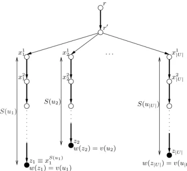
x2 1 x1 1 x2 2 x1 2 r0 r . . . z1≡ xS(u1 1) z|U | z2 w(z2) = v(u2) w(z1) = v(u1) x2 |U | x1 |U | S(u1) S(u2) _S(u |U |) w(z|U |) = v(u|U |) Fig. 1. Instance ofRTT used for the transformation from an instance of knapsack.

Knapsack

GIVEN: A finite set U , for each u ∈ U a size S(u) ∈

Z>0, a value v(u) ∈ Z>0, and positive integers B, K ∈ Z>0.

PROB.: Is there a subset U0 ⊆ U s. t.P_u∈U0S(u) ≤ B

andP_u∈U0v(u) ≥ K?

Theorem 4.1: RTTdec is N P -complete.

Proof: A solution for RTTdeccan be verified in poly-nomial time, as we only need to find out whether there exists a subtree of size bigger than ∆ where no slack time α has been added. This can be performed by counting for each node v, how many descending nodes are affected if a delay of α is assumed to occur at the in-arc of x. Starting from the leaves of the tree and moving up until the root, the procedure needs a simple visit of the tree, hence RTTdec is in N P .

Given an instance IKnapsack _{of Knapsack where U =} {u1, u2, . . . , u|U |}, we define an instance IRTT of RTTdec. See Fig. 1 for a visualization of IRTT_{. Without loss of} generality, we assume that S(ui) ≤ B, for each ui ∈ U . The set of nodes is made of: nodes r, r0 _{and the sets of} nodes Xi = {x1

i, x2i, . . . , xS(ui i) ≡ zi}, for each ui ∈ U . The set of arcs A is made of: arc (r, r0_{); arcs (r}0_{, x}1

i), for each i = 1, 2, . . . , |U |; and arcs (xj_i, xj+1_i ), for each i = 1, 2, . . . , |U | and for each j = 1, 2, . . . , S(ui) − 1.

The weight of each node in V is 0 except for nodes zi, i = 1, 2, . . . , |U |, where w(zi) = v(ui). Finally, ∆ = B + 1, α = 1 and K0₌P

ui∈Uv(ui)(S(ui) + 2) − K. It is worth

noting that the particular tree construction preserves the size of the Knapsack instance, as each path of nodes of the same weight w can be compacted and implicitly be represented by two numbers, namely, the number

of nodes of the path and the weight w of each node. This implies that each path (x1

i, x2i, . . . , xS(ui i)−1) of our construction will be represented by the pair (S(ui)−1, 0). Also the operations performed on such paths do not need the explicit representation of the tree. In particular, the check needed to verify whether a solution is feasible can be done efficiently with respect to the compacted instance.

Now we show that, if there exists a “yes” solution for Knapsack, then there exists a “yes” solution for RTTdec.

Given a “yes” solution U0 _{⊆ U for I}Knapsack_{, we define} the following solution π for IRTT_{: π(r) = 0; π(r}0_{) = 1;} π(x1

i) = 2 for each ui∈ U0 and π(x1i) = 3 for each ui 6∈ U0_{; π(x}j

i) = π(x1i) + j − 1, for each i = 1, 2, . . . , |U | and for each j = 2, 3, . . . , S(ui).

Note that, for each ui ∈ U0_{, π(zi) = S(ui) + 1} while for each ui 6∈ U0_{, π(zi) = S(ui) + 2. As the} weight of each node in V is 0 except for nodes zi, then f (π) =P|U |_i=1π(zi) · w(zi) = P_u

i∈U0(S(ui) + 1) · v(ui) +

P

ui6∈U0(S(ui) + 2) · v(ui) =

P

ui∈U(S(ui) + 2) · v(ui) −

P

ui∈U0v(ui) ≤

P

ui∈U(S(ui) + 2) · v(ui) − K = K

0_{. We} have to show that each arc in A α-affects at most ∆ nodes. As ∆ = B + 1 > S(ui), for each ui ∈ U , then all the arcs but (r, r0_{) do not α-affect more than ∆ nodes.} Moreover, for each ui6∈ U0_{, π(x}1

i) − π(r0) = 1 + α. Hence, the arc (r, r0_{) α-affects r}0 _{and nodes x}j

i for each ui ∈ U0 and for each j = 1, 2, . . . , S(ui). Then, the overall number of affected nodes is 1 +P_ui∈U0S(ui) ≤ 1 + B = ∆.

Now we show that, if there exists a “yes” solution for RTTdec, then there exists a “yes” solution for Knapsack. Given a “yes” solution π0 _{for I}RTT_{, we define a “yes”} solution π that assigns slack times only to arcs (r0_{, x}1

i), i = 1, 2, . . . , |U | as follows: π(r) = 0; π(r0_{) = 1; π(x}1

i) = 3 for each i such that π0 _{assigns at least a slack time in} the path from r0 _{to z}

i, i.e. π0(zi) − π0(r0) ≥ S(ui) + α; π(x1

i) = 2 for each i such that π0(zi) − π0(r0) < S(ui) + α; π(xj_i) = π(x1

i) + j − 1, for each i = 1, 2, . . . , |U | and for each j = 2, 3, . . . , S(ui). Note that, if π0_{is a “yes” solution} for IRTT _{then π is also a “yes” solution for I}RTT_{. In fact,} π(zi) ≤ π0_{(zi) and then f (π) ≤ f (π}0_{) ≤ K}0_{. Moreover, the} number of nodes α-affected by (r, r0_{) in π is less than or} equal to the number of nodes α-affected by (r, r0_{) in π}0_. We define a “yes” solution for IKnapsack _{as U}0 _{= {ui :} π(x1

i) = 2}. We have to show that P

u∈U0S(u) ≤ B and

P

u∈U0v(u) ≥ K. As the number of nodes α-affected

by (r, r0_{) in the solution π is less than or equal to ∆,} then ∆ ≥ 1 +P_i:π(x1

i)=2|Xi| = 1 +

P

ui∈U0S(ui). Hence

P

ui∈U0S(ui) ≤ ∆ − 1 = B. As the weight of each node

in V is 0 except for nodes zi, then f (π) = P|U |_i=1π(zi) · w(zi) =P_i:π(x1 i)=2(S(ui) + 1) · w(zi) + P i:π(x1 i)=3(S(ui) + 2)·w(zi) = P i:π(x1 i)=2(S(ui)+1)·v(ui)+ P i:π(x1 i)=3(S(ui)+

2) · v(ui) = P|U |_i=1(S(ui) + 2) · v(ui) −P_i:π(x1

i)=2v(ui)

= P_ui∈U(S(ui) + 2) · v(ui) − P_ui∈U0v(ui) ≤ K0 =

P

ui∈U(S(ui) + 2) · v(ui) − K. Hence

P

ui∈U0v(ui) ≥ K.

Corollary 4.2: RTTopt and computing Prob(RTT ) are N P -hard.

5

P

-P

T

A

Based on the dynamic programming techniques, in this section we devise a pseudo-polynomial time algorithm for RTTopt.

Let us introduce further notation. Note that, a solu-tion for RTTopt is RTT -optimal. Let T = (V, A) be an arbitrarily ordered rooted tree, i.e. for each node v we can distinguish its children, denoted as No(v), as an ar-bitrarily ordered set {v1, v2, . . ., v|No(v)|}. For an arbitrary

subtree S(v) rooted at v ∈ V , let No(S(v)) denote the set of nodes y such that (x, y) ∈ A, x ∈ S(v) and y 6∈ S(v). Clearly, when S(v) = {v}, No(S(v)) ≡ No(v). In addition, for each node v ∈ T , let T (v) be the full subtree of T rooted in v and let Ti(v) denote the full subtree of T rooted at v limited to the first (according to the initially chosen order) i children of v. Moreover, recalling that T is a weighted tree, let c(v) = P_{x∈T (v)}w(x) be the sum of the weights of the nodes in T (v) and let |T (v)| be the number of nodes belonging to T (v). Note that, the values |T (v)| and c(v) for all v ∈ V can be computed in linear time by visiting T (r) where r is the root of T . Finally, given a node v, let us denote as d(r, v) the number of arcs on the path from the root r of T and v.

In the next lemma, we prove that when the slack time of an arc (u, v) changes, all the times associated with the events in T (v) changes accordingly.

Lemma 5.1: Given a tree T , consider two feasible so-lutions π0 _{and π such that, for an arc ¯a = (u, v),} sπ0(¯a) = s_π(¯a) − α and s_π(a) = s_π0(a), for each a 6= ¯a.

Then, f (π0_{) = f (π) − αc(v).}

Proof: By construction, all the events contained in the subtree T (v) are delayed in π of α time with respect to π0 _{due to the slack time associated with arc ¯a. For each} node x ∈ T (v) then, it holds π0_{(x) = π(x) − α. Hence,} f (π0_{) = f (π) − αc(v).}

Definition 5.2: Given a feasible solution π for the RTT problem and a node v ∈ V , the ball Bπ(v) is the largest subtree rooted at v such that each node in Bπ(v) (including v) has its incoming arc a with sπ(a) = 0. Given a feasible solution π, Bπ(v) represents the set of nodes in π which are surely affected by each possible delay occurring at a = (u, v). Due to the feasibility of π, no more than ∆ nodes can belong to Bπ(v), that is |Bπ(v)| ≤ ∆. Note that, if sπ(a) = α, then Bπ(v) is empty. We say that Bπ(v) can be extended if there exists an arc (x, y) such that x ∈ Bπ(v), y 6∈ Bπ(v), w(y) > 0, and for each a ∈ A such that x ∈ Aff(a), |Aff(a)| < ∆. A ball is said maximal if it cannot be extended.

Lemma 5.3: For each instance of RTT , with ∆ ≥ 1, there exists an RTT -optimal solution such that at most one of two consecutive arcs has a slack time of α.

Proof: Suppose that there is some RTT -optimal so-lution π that assigns a slack time to both of two con-secutive arcs, i.e. there exist (x, y), (y, z) ∈ A such that sπ(x, y) = α, spi(y, z) = α, and sπ(w) = 0 for each w ∈ No(z). Then, we can define a solution π0 _such that sπ0(x, y) = α, sπ0(y, z) = 0, and spi0(z, w) = α

for each w ∈ No(z). Note that π0 _{is feasible because} |Bπ0(z)| = 1 ≤ ∆, |Bπ0(w)| ≤ |Bπ0(w)| for w ∈ No(z), and

the remaining balls are not changed. Moreover, π0_differs from π only in z. Specifically, π0_{(z) = π(x) + 2 + α, while} π(z) = π(x) + 2 + 2α, whereas, for every node w ∈ No(z), π0_{(w) = π}0_{(z)+1+α = π}0_{(y)+2+α = π(x)+3+2α = π(w).} Clearly, π0 _{remains unchanged for every other node of} T . Thus, f (π0_{) = f (π) − αw(z) ≤ f (π) because w(z) ≥ 0.} Therefore, π0 _{is a feasible solution, with cost no greater} than the optimal one, with no two consecutive arcs having a slack time α.

The above proof implies a stronger result: no RTT -optimal solution can have two consecutive arcs with a slack time α when all the events have positive weights. For arbitrary weights, there is an optimal solution that satisfies such a property. Thus, from now on, without loss of generality we can focus on optimal solutions that do not have two consecutive arcs with a slack time α.

Lemma 5.4: There exists an RTT -optimal solution π such that Bπ(v) is maximal for each v ∈ V .

Proof: By contradiction, we assume that there exists an instance such that, for an RTT -optimal solution π there exists a non empty set of nodes V which contradicts the thesis: for each v ∈ V, Bπ(v) can be extended by adding a node from No(Bπ(v)). Let v ∈ V be a node such that the distance d(r, v) from r to v is minimal. As Bπ(v) can be extended, then there exists an arc (x, y) such that x ∈ Bπ(v), y 6∈ Bπ(v) and for each a ∈ A such that x ∈ Aff(a), |Aff(a)| < ∆. It follows that π(y) = π(x)+1+α. Then, let us define π0_{as the solution derived} by setting sπ0(x, y) = 0 and sπ0(y, w) = α for each w ∈

No(y). Specifically, π0 _{assigns π}0_{(y) = π(x) + 1, π}0_{(w) =} π0_{(y)+1+α, for w ∈ N}

o(y). Clearly, π0is feasible. Indeed, |Bπ0(u)| = |Bπ(u)|+1 ≤ ∆ for each u such that x ∈ Bπ(u)

and |Bπ0(y)| ≤ |Bπ(y)| ≤ ∆. Finally, since by Lemma 5.3

sπ(y, w) = 0 for each w ∈ No(y), it holds π0_{(u) = π(u)} for each u ∈ V \ {y}. In fact, for each w ∈ No(y), π0_{(w) =} π(x)+2+α = π(w). Thus, f (π0_{) = f (π)−αw(y) and thus} f (π0_{) ≤ f (π) because w(y) ≥ 0. Repeating the above} construction for each node in V, a feasible solution is built, with cost no greater than the optimal one, such that Bπ(v) is maximal for each v ∈ V .

From now on, without loss of generality, we focus on optimal solutions with maximal balls.

As regards to compute an optimal solution for the RTToptproblem on T , it is easy to see that, when ∆ = 0, there is a trivial optimal solution ˆπ which associates to each arc a ∈ T a slack time equal to α. From now on, let

ˆ

f =P_v∈Tπ(v)w(v) denote the cost of ˆˆ π on T .

When ∆ > 0, we are now in position to describe a dynamic programming algorithm to compute an RTT -optimal solution π∗_{. Let us start deriving the slack time} on the arcs outgoing from the root r of T . Since r has no incoming arcs, it cannot be affected by any delay. Thus, r can be considered as a node having an incoming arc associated with a slack time of α. Therefore, by Lemma 5.3, for each arc a outgoing from the root r it holds sπ∗(a) = 0. Moreover, according to Lemma 5.4,

for each v ∈ No(r), π∗ _{must have a ball Bπ}

∗(v) of size

min{|T (v)|, ∆}.

In order to complete π∗_{, let us introduce the following} notations. For any RTT solution π, let fv

i(π) denote the value of the objective function P_u∈Ti(v)π(u)w(u) computed only on the nodes of Ti(v). Moreover, let fv_(π) be the objective functionP_{u∈T (v)}π(u)w(u) evaluated on T (v).

With Gv[i, j], with i, j 6= 0, we mean the maximum gain with respect to the solution ˆπ achievable with any solu-tion π that has a ball Bπ(v) of size at most j in the subtree limited to its first i children Ti(v) rooted at v, i.e. |Bπ(v)∩ Ti(v)| ≤ j. As Gv[i, j] must be the maximum gain, solu-tion π must be optimal with respect to Ti(v), and thus |Bπ(v) ∩ Ti(v)| = min{j, |Ti(v)|}. Formally, when i, j 6= 0, Gv[i, j] = maxπ{fv

i(ˆπ) − fiv(π) : |Bπ(v) ∩ Ti(v)| ≤ j} = {fv

i(ˆπ) − fiv(π∗) : |Bπ∗(v) ∩ Ti(v)| = min{j, |Ti(v)|}}.

Moreover, with Gv[0, j], for 1 ≤ j ≤ ∆, we desig-nate the maximum gain with respect to the solution ˆπ achievable with any solution π that has a ball Bπ(v) of size at most j in the subtree limited to node v, i.e. |Bπ(v) ∩ v| ≤ j. As Gv[i, j] must be the maximum gain, solution π must be optimal with respect to T0(v), and

thus |Bπ(v) ∩ T0(v)| = min{j, |T0(v)|} = 1. Thus, Gv[0, j],

for 1 ≤ j ≤ ∆ denotes the gain of a solution π∗ _that has a ball of size 1 in node v, that is π∗ _{differs from ˆπ} only for the slack time on the incoming arc a to v, i.e. sπ(a) = 0. As proved in Lemma 5.1, we can directly set Gv[0, j] = fv_{(ˆπ) − f}v_(π∗_{) = αc(v) for 1 ≤ j ≤ ∆.}

Finally, we denote with Gv[i, 0], for 0 ≤ i ≤ |No(v)|, the maximum gain with respect to ˆπ achievable with an optimal solution π∗_{that, having a slack time of α on the} incoming arc in v, must set (by Lemma 5.3) the slack time equal to 0 for each arc (v, v`), for 1 ≤ ` ≤ i. Thus, π∗_must have a ball of size min{∆, |T (v`)|} in each subtree rooted at the first i children v1, . . . , vi of v. Formally, Gv[i, 0] = Pi

`=1{fv`(ˆπ) − fv`(π∗) : |Bπ∗(v`)| ≤ min{∆, |T (v`)|}}.

Lemma 5.5: When i, j 6= 0, the gains Gv[i, j] can be recursively computed as Gv[i, j] = max0≤s<j{Gv[i − 1, j −

s] + Gvi[|No(vi)|, s]}.

Proof: By definition, let π∗ _{be an optimal solution} such that Gv[i, j] = {fv

i(ˆπ) − fiv(π∗)} and let the ball Bπ∗(v), associated with the optimal solution π∗, be of

size t = min{j, |Ti(v)|}. As trees T (vi) and Ti−1(v) are node-disjoint, Bπ∗(v) ∩ Ti−1(v) and Bπ∗(v) ∩ T (vi) are

two disjoint subtrees, which represent the balls of π∗ restricted to Ti−1(v) and to T (vi), respectively. Let s be the size of the latter ball (which can be empty), and t − s the size of the former one (which cannot be empty because contains at least the node v).

Therefore, Gv[i, j] can be rewritten as Gv[i, j] = {fv i(ˆπ) − fiv(π0)} + {fvi(ˆπ) − fvi(π00)}, where π0_{(u) =} ½ π∗_{(u) if u ∈ Ti−1(v)} ˆ π(u) otherwise, and π00_{(u) =} ½ π∗_{(u) if u ∈ T (vi)} ˆ π(u) otherwise.

Note that both π0 _{and π}00 _{must be optimal, otherwise} one can contradict the optimality of π∗ _{by using a} cut-and-paste argument. Indeed, suppose, by contradiction, that π0_{(u) is not optimal. Then, there is another solution} in Ti−1(v), say π, with |Bπ(v)| = t − s, whose gain {fv

i(ˆπ) − fiv(π)} is greater than that of π0. Substituting π0 _{with π, one can build a new solution}

π(u) =    π(u) if u ∈ Ti−1(v) π00_{(u) if u ∈ T (vi)} ˆ π(u) otherwise,

which contradicts the optimality of the solution π∗_{. Thus,} Gv[i, j] = Gv[i−1, j−s]+Gvi[|No(vi)|, s], for some s ∈ [0, j).

Finally, since it is not known in advance how the optimal ball Bπ∗_(v) is partitioned between Ti−1(v) and

T (vi), one has to check all the feasible combinations, that is: Gv[i, j] = max0≤s<j{Gv[i − 1, j − s] + Gvi[|No(vi)|, s]}.

In order to compute an RTT -optimal solution, we propose a dynamic programming algorithm which re-quires O(∆2_{n) time complexity and O(∆n) space, when}

∆ ≥ 1, whereas it requires O(n) time and O(n) space when ∆ = 0. The algorithm makes use of the two procedures SA-DPand BUILD, given below. Algorithm

SA-DP (which stands for Slack Assignment with

Dy-namic Programming) considers an arbitrarily ordered tree T in input and performs a visit of T . It uses for each node v ∈ T two matrices Gv and SOLv, both of size (No(v) + 1) × (∆ + 1). Concerning a generic node v in T and the matrix G, theSA-DPalgorithm stores in

each entry Gv[i, j] the corresponding value Gv[i, j].

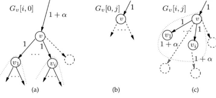
1 + α 1 ₁ v 1 v 1 Gv[i, 0] Gv[0, j] Gv[i, j] (a) (b) (c) 1 v . . . 1 + α 1 . . . . . . 1 + α vi . . . . . . vi v1 v1

Fig. 2. The three configurations that must be considered when computing matrixGv.

Fig. 2 shows the possible configurations to consider when evaluating Gv[i, j].

Note that when j > |Ti(v)|, we set Gv[i, |Ti(v)|] = Gv[i, |Ti(v)| + 1] = . . . = Gv[i, j].

If j = 0 (Fig. 2(a)), since as discussed above Gv[i, 0] = Pi

`=1{fv`(ˆπ) − fv`(π∗) : |Bπ∗(v`)| ≤ min{∆, |T (v`)|}},

we compute Gv[i, 0] =Pi<sub>`=1</sub>Gv`[|No(v`)|, ∆].

If i = 0 and j > 0 (Fig. 2(b)), by the above discussion, Gv[0, j] = αc(v), for each 1 ≤ j ≤ ∆.

Finally, if i > 0 and j > 0 (Fig. 2(c), by Lemma 5.5), Gv[i, j] = max0≤s<j{Gv[i − 1, j − s] + Gvi[|No(vi)|, s]}.

Concerning a generic node v in T and the matrix SOLv, the SA-DP algorithm memorizes in SOLv the

AlgorithmSA-DP

Input: v ∈ V

Output: SOLu, for each u ∈ T (v) 1. for i = 1 to k 2. SA-DP(vi) 3. Gv[i, 0] =Pi `=1Gv`[|No(v`)|, ∆], for 0 ≤ i ≤ No(v) 4. Gv[0, j] = αc(v), for 1 ≤ j ≤ ∆ 5. for i = 1 to k 6. for j = 1 to ∆ 7. if j ≤ |Ti(v)| then 8. Gv[i, j] = max 0≤s<j{Gv[i − 1, j − s] + Gvi[|No(vi)|, s]}

9. let s∗ _{be the index giving the maximum at Line 8} 10. SOLv[i, j] = s∗

11. else Gv[i, j] = Gv[i, j − 1] 12. SOLv[i, j] = SOLv[i, j − 1]

choices that lead to the optimal gains computed in the corresponding matrix Gv (Lines 10 and 12 of the algorithm). All matrices SOLv, v ∈ T , are first initialized by assigning 0 to each entry. Then, if i, j > 0, the entry SOLv[i, j] stores the size s of the ball Bπ(vi) rooted at the i-th child vi of v which gives the maximum gain when evaluating Gv[i, j]. Basically, if SOLv[i, j] 6= 0, then the arc (v, vi) has no slack time. Viceversa, if SOLv[i, j] = 0, either the arc (v, vi) has a slack time of α (i.e., |Bπ(vi)| = 0 that is j = 0) or such an arc does not exist (i.e., i = 0).

Now, we have to show how to construct the optimal solution π from matrices SOLv, i.e. how to assign to each v ∈ T the value π(v). Recall first that, by the discussion after Lemma 5.3, π(r) = 0 and, for each v` ∈ No(r), π(v`) = π(r) + 1 = 1. Moreover, a ball Bπ(v`) of size min = {|T (v`)|, ∆} is rooted at each v` ∈ No(r). An optimal solution is computed by calling, for each child v`∈ No(r), the procedure BUILD(v`, |No(v`)|, ∆).

AlgorithmBUILD

Input: v ∈ V , i ∈ [0, |No(v)|], j ∈ [0, ∆] 1. if i > 0 then

2. if SOLv[i, j] > 0 then

3. s := SOLv[i, j]; π(vi) := π(v) + 1 4. BUILD(vi, |No(vi)|, s)

5. BUILD(v, i − 1, j − s)

6. else

7. π(vi) := π(v) + 1 + α 8. for each w ∈ No(vi) 9. π(w) := π(vi) + 1 10. BUILD(w, |No(w)|, ∆) 11. BUILD(v, i − 1, j)

Algorithm BUILD(v, i, j) recursively builds the most

profitable ball Bπ(v) of size j with respect to Ti(v). At first, it determines the slack time on the arc (v, vi) depending on SOLv[i, j]. If SOLv[i, j] > 0, then the slack time on the arc (v, vi) is equal to 0, and the ball Bπ(v) consists of two sub-balls: one of size SOLv[i, j] in T (vi) and one of size j − SOLv[i, j] in Ti−1(v). Whereas, if SOLv[i, j] = 0, the ball of size j in the subtree T (v) does

not contain nodes in T (vi) but only in Ti−1(v). However, since the slack time on the arc (v, vi) is equal to α, by Lemma 5.3, all the arcs outgoing from vi, say (vi, wk) for 1 ≤ k ≤ |No(vi)|, have slack time equal to 0. The balls of size at most ∆ rooted at the nodes w ∈ No(vi), are recursively built by invoking |No(vi)| times Algorithm

BUILD, one for each child of vi.

Finally, we define AlgorithmSA-DP BUILDwhich

out-puts a robust timetable π by performing first SA-DP(r)

and BUILD(v`, |No(v`)|, ∆), for each v` ∈ No(r). By

construction, the following theorem can be stated.

Theorem 5.6: For any ∆ ≥ 0, SA-DP BUILD is RTT

-optimal. Moreover:

Theorem 5.7: For ∆ ≥ 1, SA-DP BUILD requires

O(∆2_{n) time and O(∆n) space. For ∆ = 0,SA-DP BUILD}

requires O(n) time and O(n) space.

Proof: The time complexity of the SA-DP

proce-dure follows by observing that, for a given v ∈ T , to fill the entry of Gv[i, j] requires O(i) time if j = 0 (Line 3), O(1) if i = 0 and j > 0 (Line 4), and O(j) if i, j > 0 (see the recurrence defined by Lines 5– 12), and hence the matrices Gv and SOLv are filled in O(|No(v)|∆2_{) time. Thus, to fill all the matrices in T , it}

costs P_v∈TO(|No(v)|∆2_{) = O(n∆}2_{). On the other side,}

procedureBUILD performs a visit of T to compute the

assignment π(v) for each node v ∈ T and thus, it takes O(n) time.

If ∆ = 0, Lines 6–12 of procedure SA-DP are not

executed and hence SA-DP only performs a visit of T

requiring O(n) time.

Theorem 5.8: For ∆ ≥ 1, Prob(RTT ,SA-DP BUILD) ≤

1 +α

2 and Prob(RTT ) ≥ 1 +∆+1α .

Proof: For the first part of the theorem, as ∆ ≥ 1,

SA-DP does not leave slack times associated to two

consecutive arcs. In fact, for any pair of consecutive arcs a = (x, y), b = (y, z) ∈ A either π(z) = π(x) + 2 or π(z) = π(x)+2+α. Then, for each v ∈ V , π(v) ≤ d(r, v)+ αbd(r,v)₂ c ≤ d(r, v)¡1 +α

2

¢

. For any optimal solution π0_of T T , π0_{(v) ≥ d(r, v). When ∆ = 0, π}0_{(v) ≥ d(r, v)α and} this is equal to the solution provided bySA-DP BUILD,

as it does not remove any slack time. Therefore, the statement holds.

Regarding the second part of the theorem, it is suffi-cient to give an instance such that any robust solution π implies f (π) ≥ (1 + α

∆+1) · f (π0), where π0 is an optimal

solution for T T . Let us consider a tree consisting of a single path of ∆+1 arcs (xi, xi+1), i = 0, 1, . . . , ∆, x0≡ r.

For each i = 0, 1, . . . , ∆, w(xi) = 0 and w(x∆+1) >

0. Each solution π of RTT is such that π(x∆+1) ≥

d(x0, x∆+1) + α = ∆ + 1 + α. An optimal solution π0 for

T T is such that π0_(x ∆+1) = d(x0, x∆+1) = ∆ + 1. Hence, f (π) = (∆+1+α)w(x∆+1) = (1+_∆+1α )·(∆+1)w(x∆+1) = (1 + α ∆+1) · f (π0).

6

E

S

We present the experimental results first on real-world data provided by Trenitalia [18] and, then, on randomly

generated data.

6.1 Real-world data

We consider real case scenarios of Single-Line Corridors. A corridor is a sequence of stations linked by multiple tracks. Each station is served by many trains of different types. Types of trains mostly concern the locations that each train serves and its maximal speed. For an example, see Figure 3. In these systems, it is a practical evidence that slow trains wait for faster trains in order to serve passengers to small stations. This situation is modelled with the only assumption that the changes of passengers from one train to another at a station must be guaranteed only when the second train is starting its journey from the current station. In practice, the only restriction is that we do not require as a constraint the possibility for passengers to change for a train which has already started its journey. This does not mean that passengers cannot change train at some station in the middle of a train journey, but only that this is not considered as a constraint. Further motivations for this model can be found in [6], [7].

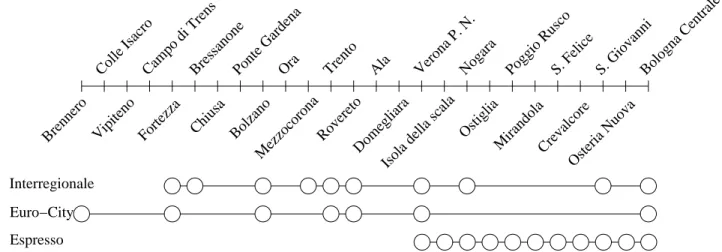
Let us consider the real-world example provided in Figure 3 where three trains serve the same line. The slowest train, the Espresso, goes from Verona to Bologna, the Interregionale goes from Fortezza to Bologna, and the fastest one, the Euro-City, goes from Brennero to Bologna.

The Euro-City starts its journey before all the other trains, and it arrives at Fortezza station before the depar-ture event of the Interregionale. At Verona Station, the Espresso is scheduled to start its journey after the arrival event of the Euro-City. Hence, there is an arc between the Euro-City and the starting event corresponding to the Interregionale at Fortezza station, and another arc connecting the Euro-City to the starting event of the Espresso at Verona station. As described above, an arc which represents a changing activity can only connect one node to the head of a branch. The DAG obtained by this procedure is a tree, as shown in Figure 3. In general, the result of this procedure is a forest and we link the roots of the trees in this forest to a unique root event. The weights on the events are assigned according to the relevance of the trains which they belong to, and the weight of the root is 0. The rationale behind such a choice is given by the priority that faster trains have with respect to the slower ones, and to the fact that they also serve more passengers. Another interest-ing weightinterest-ing function could be to associate different weights to different events according to the number of involved passengers. Unfortunately, this would require more precise input data than that we could retrieve.

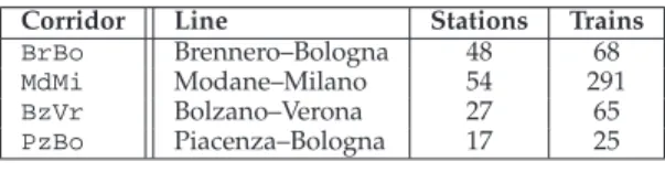
Table 1 shows the data used in the experiments re-ferring to 4 corridors provided by Trenitalia. Starting from the provided data and according to the described requirements, we derived event activity networks having tree topologies whose sizes are reported in Table 2. We

Corridor Line Stations Trains

BrBo Brennero–Bologna 48 68

MdMi Modane–Milano 54 291 BzVr Bolzano–Verona 27 65

PzBo Piacenza–Bologna 17 25

TABLE 1

Data used in the experiments.

then apply theSA-DP BUILDalgorithm on different

sce-narios, comparing the obtained robust timetables with the optimal non-robust ones.

Corridor N. of Max. time Avg activity Max. N.

nodes of traveling time of hops

BrBo 1103 516 9 66

MdMi 4358 318 8 27

BzVr 648 197 5 37

PzBo 163 187 10 14

TABLE 2 Sizes of the trees.

We now show and discuss interesting results about the applicability and the low costs in terms of slack times needed for making robust the considered timetables with respect to different scenarios.

Our experiments are based on three main parameters. Namely, we vary on the maximum number ∆ of events that can be affected by an occurring delay, the maximum time delay α, and the case of average or real times L needed to perform the scheduled activities. In what fol-lows, all the activities times and the delays are expressed in minutes.

In order to obtain RTT instances, for each corridor among BrBo, MdMi, BzVr and PzBo, we vary ∆ ∈

[1, 2, . . . , 1000] and α ∈ {1, 5, 9, 13, 17}. Moreover, we use two different functions L: the first one is based on the real values obtained by available data; the second one is the constant average function which assigns to each activity the same duration time obtained as the average among all real values of each instance. This second function is used to test the behavior of the algorithm based only on the tree network topology, in order to understand the dependability with respect to real values. The average activity times for each instance are shown in Table 2.

For each corridor we show three diagrams concerning the objective function f , the price of robustness Prob of

SA-DP BUILD, and the computational time t needed by

SA-DP BUILDin the mentioned cases. In each diagram,

we show three curves which represent the results ob-tained by setting L to real values and α ∈ {1, 5, 9}. Results obtained by assigning α ∈ {13, 17} are not shown as they are less significant being α too large compared with the average activity time. Furthermore, for the instance BrBo, we give the three diagrams obtained by

setting L to the corresponding average activity time. For any other instance we do not give these diagrams as

Brennero

Colle Isacro

Osteria Nuova Crevalcore Isola della scala

Domegliara Rovereto Mezzocorona Fortezza Mirandola Ostiglia Bolzano Chiusa Vipiteno

Campo di TrensBressanonePonte GardenaOra Trento Ala Verona P. N.Nogara Poggio RuscoS. Felice S. GiovanniBologna Centrale

Espresso Euro−City Interregionale

Fig. 3. Example of three trains serving a same line. For the sake of clarity, for each station and for each train, we represented only one circle which indeed corresponds to an arrival and a departure event.

Euro−City Interregionale

Espresso

Fig. 4. A tree obtainable from the example provided by Figure 3.

α = 9 α = 5 α = 1 ∆ Prob 1000 100 10 1 5.5 5 4.5 4 3.5 3 2.5 2 1.5 1

Fig. 5. Theoretical lower bounds toProb.

the inferred properties do not change. The full set of results can be found in [1]. All the experiments have been carried out on a workstation equipped with a 2,66 GHz Intel Core2 processor, 8Gb RAM, Linux (kernel 2.6.27) and gcc 4.3.3 compiler.

In the obtained diagrams, the values of the objective function f of the robust problem are compared to the optimum, i.e. the value of f given by the non-robust problem. As ∆ increases, the curves tend rapidly to the optimum. For small values of α, the price of robustness is very low.

In order to compare the experimentally computed values of Prob with the theoretical lower bounds given by Theorem 5.8, we provide Figure 5 which shows the values of function 1 + α

∆+1 for α ∈ {1, 5, 9} and

∆ ∈ [1, . . . , 1000]. Note that, the computed values of Prob are always smaller than the theoretical lower bounds as the latter are given for the worst case instances.

Concerning the diagrams representing the computa-tional times, we can see that our tests required a very small amount of time. The linear growth of the curves as ∆ increases is evident. For practical purposes, our experiments show that algorithm SA-DP BUILD can be

safely applied without requiring ages of computation.

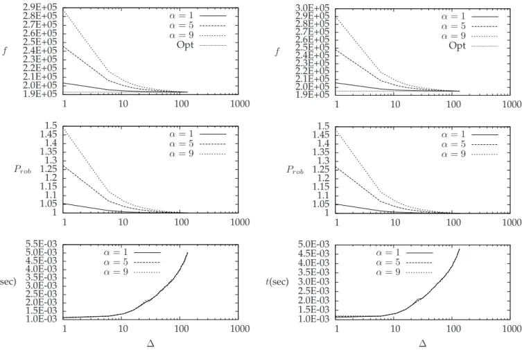
6.1.1 CorridorBrBo(see Figure 6)

This corridor is quite large in terms of served stations and passing trains as shown in Table 1. We can see that the price of robustness is very close to 1 when α = 1 while it is almost 1.5 when considering big delays of α = 9 and ∆ = 1.

When ∆ = 1, the algorithm adds one slack time for each pair of consecutive arcs. As shown in Figure 6, the value of Prob, when ∆ = 1, is about 2Lavg+α

2Lavg = 1 +

α

2Lavg,

where Lavg is the average activity time.

It is also interesting to note how the values of f and Prob decrease quickly with ∆. In particular, the price of robustness is 1 when ∆ = 136 and α = 9, that is that with ∆ = 136 we do not have to pay for introducing robustness. As a special case, we mention that the price of robustness is between 1.00754 and 1.06785, when ∆ = 11. This implies that adding robustness reflects an increasing in the costs of just 0.7 − 6.7% even for a small value of ∆.

Regarding the computational time, we can see that it increases with ∆ but it is less than 5 milliseconds in the worst case (i.e. when α = 9 and ∆ = 136). In detail, in the worst case, for ∆ = 136 we need about 5.01 milliseconds to achieve a price of robustness of 1.

α = 9 α = 5 α = 1 ∆ t(sec) 1000 100 10 1 5.5E-03 5.0E-03 4.5E-03 4.0E-03 3.5E-03 3.0E-03 2.5E-03 2.0E-03 1.5E-03 1.0E-03 α = 9 α = 5 α = 1 Prob 1000 100 10 1 1.5 1.45 1.4 1.35 1.3 1.25 1.2 1.15 1.1 1.05 1 Opt α = 9 α = 5 α = 1 f 1000 100 10 1 2.9E+05 2.8E+05 2.7E+05 2.6E+05 2.5E+05 2.4E+05 2.3E+05 2.2E+05 2.1E+05 2.0E+05 1.9E+05

Fig. 6. CorridorBrBowith real values of minimum activity times

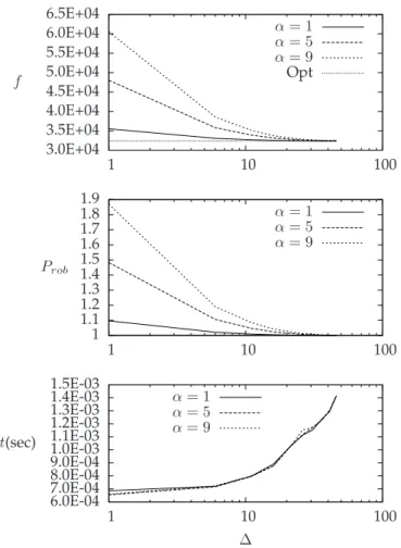
6.1.2 Corridor BrBo (average activity times) (see

Fig-ure 7)

In this case, the objective function assumes almost iden-tical values with respect to the previous case. As we expect, the value of the objective function does not depend on the value of L, but only on the structure of the tree and on the size of the delay.

Regarding Prob, its value strictly depends on α/Lavg which can be considered a parameter for evaluating the magnitude of a delay. It is worth noting that for ∆ = 1 an optimal robust timetable has to assign exactly one slack time of size α for each pair of consecutive activities. It follows that, when α = 9 and the average activity time is equal to 9, the price of robustness is 1.5, as it can be verified in Figure 7. The same happens for α = 5, where the expected value is about 1.27.

6.1.3 CorridorMdMi(see Figure 8)

This corridor is the biggest in terms of served stations and passing trains. As shown in Table 1, the number of considered trains is more than four times the one in BrBo, while the number of stations is slightly more.

Still, we can see comparable performances with respect to the price of robustness (it is 1 for each ∆ ≥ 966) even though the incidence of the required computational time

α = 9 α = 5 α = 1 ∆ t(sec) 1000 100 10 1 5.0E-03 4.5E-03 4.0E-03 3.5E-03 3.0E-03 2.5E-03 2.0E-03 1.5E-03 1.0E-03 α = 9 α = 5 α = 1 Prob 1000 100 10 1 1.5 1.45 1.4 1.35 1.3 1.25 1.2 1.15 1.1 1.05 1 Opt α = 9 α = 5 α = 1 f 1000 100 10 1 3.0E+05 2.9E+05 2.8E+05 2.7E+05 2.6E+05 2.5E+05 2.4E+05 2.3E+05 2.2E+05 2.1E+05 2.0E+05 1.9E+05

Fig. 7. CorridorBrBowith average activity times

becomes more evident. However, as the timetables are calculated at the planning phase and not at runtime, the required time is still of an acceptable order being about 192.88 milliseconds in the worst case.

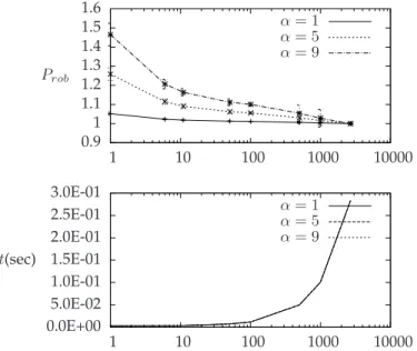
6.1.4 CorridorsBzVrandPzBo(see Figures 9 and 10)

As expected, for the small corridorsBzVrandPzBo, the

price of robustness tends to the optimum much faster than for the other cases. Moreover the time required for the computations is negligible (in the worst cases, it is 1.41 milliseconds forBzVrand 0.27 milliseconds for PzBo).

For corridor BzVr, the price of robustness for small

values of ∆ is high, whereas, it is small for corridor

PzBo. This is due to the fact that in the former case the

average activity time is much smaller than the value of α, while in the latter case the average activity time is always greater than α.

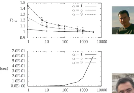
6.2 Randomly generated data

By analyzing the results in the previous section, it is worth noting that the price of robustness tends to 1 faster than one would expect by the theoretical bounds (see Theorem 5.8 and Figure 5). This suggests that those instances have some hidden properties. One cause might

α = 9 α = 5 α = 1 ∆ t(sec) 1000 100 10 1 2.0E-01 1.8E-01 1.6E-01 1.4E-01 1.2E-01 1.0E-01 8.0E-02 6.0E-02 4.0E-02 2.0E-02 0.0E+00 α = 9 α = 5 α = 1 Prob 1000 100 10 1 1.5 1.45 1.4 1.35 1.3 1.25 1.2 1.15 1.1 1.05 1 Opt α = 9 α = 5 α = 1 f 1000 100 10 1 8.5E+05 8.0E+05 7.5E+05 7.0E+05 6.5E+05 6.0E+05 5.5E+05

Fig. 8. CorridorMdMi

be the almost linearity of the tree structure, that is, the trees are made of long paths and the nodes have low outdegree.

In order to investigate on this matter, we test the behavior of the algorithm on three sets of five ran-domly generated trees: Random1000,Random3000and

Random5000, containing five trees of 1000, 3000 and

5000 nodes, respectively. Each tree is generated starting from a single node and then by linking a new generated node to an existing one extracted uniformly at random. The node weights randomly rank between 1 and 10, and the minimum duration time for each activity randomly ranks between 1 and 18. In this way, the average activity duration time is comparable with that of the presented real-world instances. Finally, ∆ ∈ [1, 2, . . . , 10000] and α ∈ {1, 5, 9}. For each pair (∆, α), we performed one test for each randomly generated tree.

In Figures 11, 12, and 13, we summarize the obtained results. In particular, we show the average values of the price of robustness and the computational time, and the standard deviation of the price of robustness. The ob-tained results confirm our intuition that the almost linear structure of the real-world data heavily influences the curve of the price of robustness, while the computational time is not affected.

This is evident if we compare the results of graphs

α = 9 α = 5 α = 1 ∆ t(sec) 100 10 1 1.5E-03 1.4E-03 1.3E-03 1.2E-03 1.1E-03 1.0E-03 9.0E-04 8.0E-04 7.0E-04 6.0E-04 α = 9 α = 5 α = 1 Prob 100 10 1 1.9 1.8 1.7 1.6 1.5 1.4 1.3 1.2 1.1 1 Opt α = 9 α = 5 α = 1 f 100 10 1 6.5E+04 6.0E+04 5.5E+04 5.0E+04 4.5E+04 4.0E+04 3.5E+04 3.0E+04 Fig. 9. CorridorBzVr

inRandom1000(Figure 11) with those of corridorBrBo

(Figures 6) which have comparable size. In fact, we can see that the computational time is almost identical (when ∆ = 136, it is 3.53 milliseconds for Random1000 and

5.01 milliseconds for BrBo) but the price of robustness

ofRandom1000is 1 only if ∆ ≥ 876, while for BrBo the

price of robustness is 1 for each ∆ ≥ 136.

The same observation can be done by comparing

Random5000with corridorMdMi. In this case, the price

of robustness of MdMi is 1 for each ∆ ≥ 966 while the

price of robustness of Random5000 is 1 only if ∆ ≥

3746. The computational times are still very close being 192.88 milliseconds forMdMiand 162.04 milliseconds for

Random5000, when ∆ = 966.

7

C

We have presented the problem of planning robust timetables when the input event activity network topol-ogy is a tree. The delivered timetables can cope with one possible delay that might occur at runtime among the scheduled activities. In particular, our algorithms ensure that if a delay occurs, no more than ∆ activities are affected by the propagation of such a delay. We have proved that the problem is N P -hard but not in the strong sense as it is pseudo-polynomially solvable.

α = 9 α = 5 α = 1 ∆ t(sec) 100 10 1 2.8E-04 2.6E-04 2.4E-04 2.2E-04 2.0E-04 1.8E-04 1.6E-04 1.4E-04 α = 9 α = 5 α = 1 Prob 100 10 1 1.45 1.4 1.35 1.3 1.25 1.2 1.15 1.1 1.05 1 Opt α = 9 α = 5 α = 1 f 100 10 1 1.4E+04 1.4E+04 1.3E+04 1.2E+04 1.2E+04 1.2E+04 1.1E+04 1.0E+04 1.0E+04 9.5E+03

Fig. 10. CorridorPzBo

Although the combinatorial optimization problem arisen by our study is of its own interest, the paper continues the recent study on robust optimization theory. This is an important rising field led by the necessity of managing unpredictable limited disruptions with limited resources.

Several directions for future works deserve investiga-tion such as the analysis of different recovery strategies, the application of other modification functions to the ex-pected input and the enforcement of the recoverable ro-bustness to other fundamental optimization problems.

R

[1] http://informatica.ing.univaq.it/misc/TimetablingTree2009/.

[2] S. Cicerone, G. D’Angelo, G. Di Stefano, D. Frigioni, and A. Navarra. Robust Algorithms and Price of Robustness in Shunt-ing Problems. In ProceedShunt-ings of the 7th Workshop on Algorithmic

Approaches for Transportation Modeling, Optimization, and Systems (ATMOS07), pages 175–190, 2007.

[3] S. Cicerone, G. D’Angelo, G. Di Stefano, D. Frigioni, and A. Navarra. Delay Management Problem: Complexity Results and Robust Algorithms. In Proceedings of the 2nd Annual

Inter-national Conference on Combinatorial Optimization and Applications (COCOA), volume 5165 of Lecture Notes in Computer Science, pages

458–468. Springer, 2008.

[4] S. Cicerone, G. D’Angelo, G. Di Stefano, D. Frigioni, and A. Navarra. Recoverable robust timetabling: Complexity results and algorithms. Journal of Combinatorial Optimization, 18(3):229– 257, 2009. α = 9 α = 5 α = 1 t(sec) 1000 100 10 1 3.0E-02 2.5E-02 2.0E-02 1.5E-02 1.0E-02 5.0E-03 0.0E+00 α = 9 α = 5 α = 1 Prob 1000 100 10 1 1.5 1.45 1.4 1.35 1.3 1.25 1.2 1.15 1.1 1.05 1 0.95

Fig. 11. Random1000: randomly generated trees with 1000 nodes α = 9 α = 5 α = 1 t(sec) 10000 1000 100 10 1 3.0E-01 2.5E-01 2.0E-01 1.5E-01 1.0E-01 5.0E-02 0.0E+00 α = 9 α = 5 α = 1 Prob 10000 1000 100 10 1 1.6 1.5 1.4 1.3 1.2 1.1 1 0.9

Fig. 12. Random3000: randomly generated trees with 3000 nodes

[5] S. Cicerone, G. D’Angelo, G. Di Stefano, D. Frigioni, A. Navarra, M. Schachtebeck, and A. Sch¨obel. Robust and Online Large-Scale

Optimization – Models and Techniques for Transportation Systems,

vol-ume 5868 of Lecture Notes in Computer Science, chapter Recoverable Robustness in Shunting and Timetabling, pages 28–60. Springer Berlin, 2009.

[6] G. D’Angelo, G. Di Stefano, and A. Navarra. Evaluation of recoverable-robust timetables on tree networks. In Proceedings

of the 20th International Workshop on Combinatorial Algorithms (IWOCA), volume 5874 of Lecture Notes in Computer Science, pages

24–35. Springer, 2009.

[7] G. D’Angelo, G. Di Stefano, and A. Navarra. Recoverable-robust timetables for trains on single-line corridors. In Proceedings of

the 3rd International Seminar on Railway Operations Modelling and Analysis (RailZurich), 2009.

[8] G. D’Angelo, G. Di Stefano, A. Navarra, and Cristina M. Pinotti. Recoverable Robust Timetabling on Trees. In Proceedings of the 3rd