Predictive model in the presence of missing data: the centroid criterion for variable selection

(1)

HAL Id: hal-01878388

https://hal.archives-ouvertes.fr/hal-01878388

Preprint submitted on 21 Sep 2018

HAL is a multi-disciplinary open access archive for the deposit and dissemination of sci-entific research documents, whether they are pub-lished or not. The documents may come from teaching and research institutions in France or abroad, or from public or private research centers.

L’archive ouverte pluridisciplinaire HAL, est destinée au dépôt et à la diffusion de documents scientifiques de niveau recherche, publiés ou non, émanant des établissements d’enseignement et de recherche français ou étrangers, des laboratoires publics ou privés.

Predictive model in the presence of missing data: the

centroid criterion for variable selection

Jean Gaudart, Pascal Adalian, George Leonetti

To cite this version:

Jean Gaudart, Pascal Adalian, George Leonetti. Predictive model in the presence of missing data: the centroid criterion for variable selection. 2018. �hal-01878388�

(2)

Predictive model in the presence of missing data: the

centroid criterion for variable selection

Jean Gaudart1§, Pascal Adalian2, George Leonetti2,3

1_{Aix Marseille Univ, IRD, INSERM, SESSTIM, Faculty of Medicine, 13005}

Marseille, France.

2_{Anthropology Unit, UMR. 6578 C.N.R.S./University of Aix-Marseille, Faculty of}

Medicine, 27 bd J. Moulin 13385 Marseille cedex 5, France.

3_{Service of Legal Medicine, Faculty of Medicine, 27 bd J. Moulin 13385 Marseille}

cedex 5, France.

Keywords: Data analysis, variable selection, missing data, centroid.

§_{Corresponding author}

Email addresses:

J Gaudart: jean.gaudart@univ-amu.fr

P Adalian: pascal.adalian@univ-amu.fr

(3)

Abstract

Introduction

In many studies, covariates are not always fully observed because of missing data process. Usually, subjects with missing data are excluded from the analysis but the number of covariates can be greater than the size of the sample when the number of removed subjects is high. Subjective selection or imputation procedures are used but this leads to biased or powerless models.

The aim of our study was to develop a method based on the selection of the nearest covariate to the centroid of a homogeneous cluster of covariates. We applied this method to a forensic medicine data set to estimate the age of aborted fetuses.

Analysis

Methods

We measured 46 biometric covariates on 50 aborted fetuses. But the covariates were complete for only 18 fetuses.

First, to obtain homogeneous clusters of covariates we used a hierarchical cluster analysis.

Second, for each obtained cluster we selected the nearest covariate to the centroid of

the cluster, maximizing the sum of correlations 



p k

jk j

g r

C max (the centroid

criterion).

Third, with the covariate selected this way, the sample size was sufficient to compute a classical linear regression model.

(4)

We have shown the almost sure convergence of the centroid criterion and simulations were performed to build its empirical distribution.

We compared our method to a subjective deletion method, two simple imputation methods and to the multiple imputation method.

Results

The hierarchical cluster analysis built 2 clusters of covariates and 6 remaining covariates. After the selection of the nearest covariate to the centroid of each cluster, we computed a stepwise linear regression model. The model was adequate

(R2_{=90.02%) and the cross-validation showed low prediction errors (2.23 10}-3_).

The empirical distribution of the criterion provided empirical mean (31.91) and median (32.07) close to the theoretical value (32.03).

The comparisons showed that deletion and simple imputation methods provided models of inferior quality than the multiple imputation method and the centroid method.

Conclusion

When the number of continuous covariates is greater than the sample size because of missing process, the usual procedures are biased. Our selection procedure based on the centroid criterion is a valid alternative to compose a set of predictors.

(5)

Introduction

Predictive models are widely used in life sciences. For clinical practice, usual statistical models like regression models are often build using observed covariates to estimate the value of a dependant variable. Particularly in anthropology and forensic sciences, predictive models are mostly used to predict age and gender of subjects from different biometrics covariates. However, all covariates are not always fully observed since data measurements can be difficult (for example in case of superposition in radiographs) and because forensic specialists frequently have to deal with incomplete human remains. Usually, subjects with missing data are excluded from the analysis (Complete-Case Analysis). But first, if the missing data depend on a non-random process related to the dependant variable, excluding this selective group leads to biased models [1]. Second, this practice reduces the statistical power of the analysis. Third, in some situations the number of removed subjects is unacceptably high: even if the missing rates per covariate are low, few subjects may have complete data for all covariates leading to analyze a number of covariates greater than the size of the sample with complete data. Then, statistical analysis and result interpretation are tricky: usual statistical methods like stepwise regression methods are not able to select the predictive covariates. To compose a set of predictors in this context, covariates are often selected via ad hoc and subjective means mostly based on the number of available data for each covariate leading to biased models.

To avoid this problem imputation methods consist on substituting the missing data with plausible values. The most popular simple imputation practice is the unconditional mean substitutions where missing data are replaced by the mean

) X (

(6)

preserves the observed sample means but under-estimates variances and covariances. Another simple imputation method substitutes each missing data by conditional means estimated from regression models (e.g. linear regression) where the covariate

Xj is estimated using the dependant variable Y (E~(X_j / Y )  f~(Y )) or other

covariates (E~(X_j / Y,X_k,X_l)  f~(Y,X_k,X_l)). But this practice biases again the models over-estimating the correlations. Another method called multiple imputations has been used in several applications [4, 5, 1, 6, 7, 8]. This technique generates imputations using Expectation-Maximization (EM) algorithm or Data Augmentation (DA) algorithm [9]. The results are combined taking into account the imputation uncertainty. However, missing data are generated from models based on the observed data and therefore multiple imputation increases colinearity [3].

The aim of this study was to develop, in this context, a method to select covariates using neither imputations nor subjective procedures and reducing amounts of information to be discarded. This method is based on the selection of the nearest covariate to the centroid of a homogeneous cluster of covariates. This selected covariate minimizes the distance to the other covariates and therefore a large amount of the cluster information is preserved. We applied this method to a forensic medicine data set in order to estimate the age of aborted fetuses.

(7)

Analysis

1. Material and methods

In case of abortions caused by traumatic situations, the fetal age has to be accurately determined. Indeed, in the french law the judgment and the prejudice appreciation differ in step with the fetal age. Fetal age can be determined using thigh-bone lengths [10] or foot lengths [11] as well as cranium bones measures. For the latter procedure of determination, 46 biometric covariates were measured (cranium bone lengths or angular measures [12, 13]) on 50 aborted fetuses. But, because of the traumatic situations, it was not possible to measure all the covariates on the whole fetus sample. The measures were complete for only 18 fetuses.

First, to obtain homogeneous clusters of covariates we used a hierarchical cluster analysis using Pearson correlations as similarity measures.

Second, for each obtained cluster of covariates we selected the nearest covariate to the centroid of the cluster. We have determined that the nearest covariate to the centroid is the covariate which maximizes the sum of correlations. Indeed [appendix 1], the squared distance between a covariate and the centroid is given by the Torgerson formula [14, 15]:

 

2

 

2

 

₂ 2 .,. 2 1 ,. , p p j j       , Where

 

1_jk



is the squared distance between two covariates, where jk is the

(8)

Then

 





k jk j j j max min2 , 

Furthermore, we have shown that this criterion 



p k

jk j

g r

C max converges almost

surely [appendix 2].

Third, with the covariate selected this way, the sample size was sufficient to compute a stepwise linear regression model. The results were analyzed by cross-validation procedure and goodness-of-fit was estimated by the rate of explained variability R².

In the presented statistical context (finite sample size and jk0), the distribution of

the empirical correlation coefficient, rjk, is not simply usable [16, 17]. Then, it is not

possible to formalize the distribution of the maximum of the empirical correlation

sum ( 



p k jk j g r

C max ). Therefore we studied the empirical distribution of Cg by

simulations. Using the variance-covariance matrix of a cluster of p covariates issued from our sample, we simulated the same number p of covariates. Those covariates were extremely correlated and were normally distributed. To determine the number of simulations, we used, for each centile, the relative errors between a centile c ;

 

i n

(9)

We compared the resulting model with 4 other methods:

i. The deletion procedure deleting covariates until the sample size is greater than the number of covariates;

ii. The simple unconditional mean imputation method, imputing the estimated mean of each covariate to missing data (for each covariate Xj: E~(X _j ));

iii. The simple conditional mean imputation method, imputing to missing data the predicted value resulting from a simple linear regression on the variable Age (for each covariate Xj: E~(X_j / Age) ~~Age );

iv. The multiple imputation method: to generate imputations we used the DA algorithm (broadly described by 9). For this purpose, Schaffer's Norm® freeware was employed. Missing values were replaced by 20 simulated values in order to assure the efficiency of the procedure [2]. The 20 sets of imputations reflected the uncertainty about the true values of missing data. Each of the 20 completed data sets was analyzed using standard linear regression method. The results were combined into a single inference according to the procedure described for example in [9] [2] or [4].

The datasets, obtained by these four methods, were analyzed by stepwise linear regression. The goodness-of-fits of the resulting models were compared using the rates of explained variability and the accuracies were compared by the prediction errors provided by cross-validations.

(10)

2. Results

2.1. Centroid method of selection

The hierarchical cluster analysis (fig. 1), using 46 covariates, built 2 clusters with respectively 36 and 4 clustered covariates. The 6 remaining covariates (AFW: Weisbach angle, APN: nasal angle, ATO: foramen magnum angle, ASP: nasion-sphenion-basion angle, NKB: nasion-klition-basion angle, ABO: angle formed by the straight line nasion-opisthion and the Francfort section) appeared to be separate from

the other covariates. In the first cluster (36 covariates) the Cg criterion allowed us to

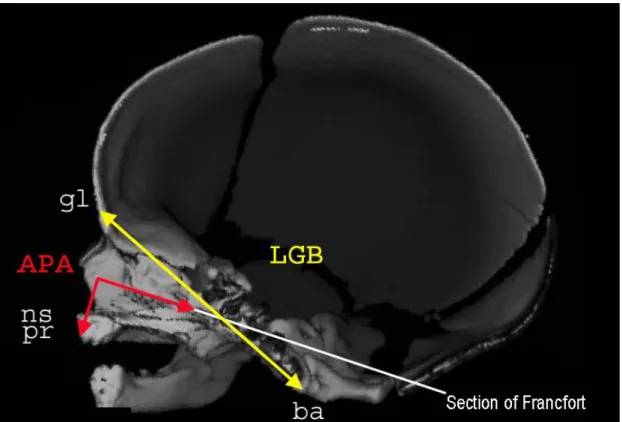
select the covariate called LGB (glabella-basion length). That is, this covariate maximized the correlation sum and therefore was the nearest covariate to the centroid of the first cluster. The covariate LGB (fig. 2) represents the length between the frontal bone and the foramen magnum. This length is a usual and standardized measure [18] and, for fetuses, LGB can be easily measured by scanner. In the same way, the Cg criterion allowed us to select the covariate called APA (alveolar profile

angle [13, 18]) in the second cluster composed of 4 covariates.

On the whole we obtained 8 covariates with a sample size of 35 fetuses (free of missing data) to compute a stepwise linear regression model. We obtained the following model (fig. 3):

LGB .

.

age 484  0696

(age in weeks of amenorrhea, LGB in millimeter).

The model was adequate (R2=90.02%) and the cross-validation showed very low

(11)

Figure 1: hierarchical cluster analysis using the correlation coefficient of Pearson as

similarity measure. We obtained 2 homogeneous clusters of covariates and 6 remaining covariates.

(12)

APA: alveolar profile angle

gl: glabella: most anterior midline point of the frontal bone, usually above the

frontonasal suture.

ns: nasospinal: intersection between the midline and the tangent to the margin

of the inferior nasal aperture, at the lowest points.

pr: prosthion: midline point of the most anterior point of the maxillae alveolar

process.

ba: basion: midline point of the anterior margin of the foramen magnum.

Figure 3: scatter plot of the age (in weeks of amenorrhea) and the LGB (in

millimeter).

(13)

2.2. Simulations

Using the variance-covariance matrix of the first homogeneous cluster of covariates, we simulated 36 correlated and normally distributed covariates.

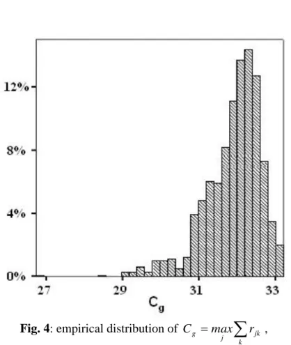
With 1000 simulations (fig. 4) the empirical distribution of Cg was stable that is the

relative errors of each centile were lower than 0.02. The empirical mean (31.91 CI95% [31.86; 31.96]) and the empirical median (32.07) were close to the theoretical value (32.03) in spite of the small size of the simulated samples (n=18 subjects). The

empirical variance (0.56) and the empirical range (minimum=26.75;

maximum=33.22) were also small.

Fig. 4: empirical distribution of 



k

jk j

g max r

C ,

(14)

2.3. Comparisons

The four other methods provided four different groups of selected covariates. These groups were analyzed using stepwise linear regression procedure.

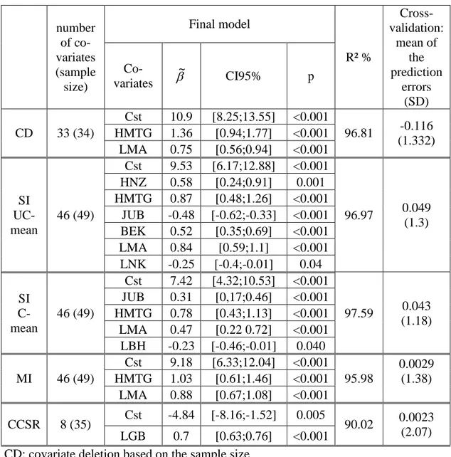
i. The first method provided covariate deletions based on the sample size: covariates composed of the larger number of missing data were deleted until the size of the sample (with complete data) was greater than the number of covariates. We obtained 33 fully observed covariates for 34 subjects. Stepwise linear regression provided a linear model composed of 2 covariates (HMTG: mastoid height and LMA: maxillo-alveolar length) (table 1). The rate of explained variability R² was important (96.81%) but cross validation provided non-negligible prediction errors (mean:-0.116 CI95%[-0.564;0.332]).

ii. The analysis of the sample completed with simple imputations of unconditional means provided a linear model composed of 6 covariates (HNZ: nasal height, HMTG, JUB: bijugal breadth, BEK: biorbital breadth, LMA, LNK: nasion-klition length). The R²-value was important 96.97% and cross validation provided low prediction errors (mean: 0.049 CI95%[-0.32;0.41]) (table 1).

iii. With the simple imputation method imputing conditional means (estimated from simple linear regression models) to missing data, stepwise linear regression procedure provided a final predictive model composed of 4 covariates (JUB, HMTG, LMA, LBH: basion-hormion length). The goodness-of-fit criterion R² was high (97.59%) and cross validation provided low prediction errors (mean: 0.043 CI95%[-0.29;0.37]) (table 1).

(15)

iv. Finally, the multiple imputation method provided a model composed of 2 covariates (HMTG, LMA). The value (95.98%) was slightly lower than the R²-values of the latter models but the cross validation provided very low prediction errors (mean: 0.0029 CI95% [-0.38;0.39]).

Table 1: Results of the four modeling procedures.

number of co-variates (sample size) Final model R² % Cross-validation: mean of the prediction errors (SD) Co-variates  ~ CI95% p CD 33 (34) Cst 10.9 [8.25;13.55] <0.001 96.81 -0.116 (1.332) HMTG 1.36 [0.94;1.77] <0.001 LMA 0.75 [0.56;0.94] <0.001 SI UC-mean 46 (49) Cst 9.53 [6.17;12.88] <0.001 96.97 0.049 (1.3) HNZ 0.58 [0.24;0.91] 0.001 HMTG 0.87 [0.48;1.26] <0.001 JUB -0.48 [-0.62;-0.33] <0.001 BEK 0.52 [0.35;0.69] <0.001 LMA 0.84 [0.59;1.1] <0.001 LNK -0.25 [-0.4;-0.01] 0.04 SI C-mean 46 (49) Cst 7.42 [4.32;10.53] <0.001 97.59 0.043 (1.18) JUB 0.31 [0,17;0.46] <0.001 HMTG 0.78 [0.43;1.13] <0.001 LMA 0.47 [0.22 0.72] <0.001 LBH -0.23 [-0.46;-0.01] 0.040 MI 46 (49) Cst 9.18 [6.33;12.04] <0.001 95.98 0.0029 (1.38) HMTG 1.03 [0.61;1.46] <0.001 LMA 0.88 [0.67;1.08] <0.001 CCSR 8 (35) Cst -4.84 [-8.16;-1.52] 0.005 90.02 0.0023 (2.07) LGB 0.7 [0.63;0.76] <0.001

CD: covariate deletion based on the sample size

SI UC-mean: simple unconditional mean imputations to missing data

SI C-mean: simple conditional mean imputations (conditioned by Age), estimated from simple linear regression model, to missing data.

MI: multiple imputations.

CCSR: centroid method for covariate space size reduction.

Cst: model's constant, ~: estimation of the coefficients of the linear model. p: p-value testing the coefficients to zero (t-test)

(16)

3. Discussion

When the number of continuous covariates is greater than the sample size, because of missing data process, imputations methods or ad hoc selections based on available data are commonly applied. Our study showed that in this context the selection method based on the centroid criterion is a valid alternative method. Indeed, the choice of the nearest covariate to the centroid of a cluster of covariates is a simple selection method which avoids resorting to imputations or ad hoc selections.

Complete Case Analysis cannot be applied and the covariate selection based on the sample size is not accurate as this method leads to biased models with high prediction errors. Simple imputation methods involve well-known biases [1, 2, 3, 9]. Unconditional mean imputations provide underestimated variances and covariances and introduce a conservative bias reducing the strength of the relationship between the

dependant variable Y and the covariates Xj completed this way. Conditional mean

imputations provide overestimated correlations and over-fitted models. This method introduces costly bias increasing the strength of the relationship between the

completed covariates Xj and the dependant variable Y. On the other hand, the multiple

imputation procedure provided here the best model according to goodness-of-fit and prediction errors. Performing 20 imputations lead to an efficiency of 96.9% in the presence of more than 50% of missing data [2]. But MI is known to increase colinearity [1, 2, 3, 4, 9, 19]. It introduces a costly bias increasing the strength of the relationship between the dependant variable Y and the completed predictive covariates

Xj. Furthermore, different MI procedures can lead to different inferences [7]. Even if

multiple imputation method does not much disturb the results of an explicative model (i.e. the presence or absence of relationship between the dependant variable and the covariates) imputations do modify predictions [6]. The selection method based on the

(17)

centroid criterion is a good alternative finding an accurate model: even if the results displayed the lowest goodness-of-fit, the latter remained high (R²=90.02%) and cross validation provided the lowest prediction errors mean: 0.0023 CI95% [-0.58;0.58]). Missing data do not disturb our selection method as far as they are missing at random. The correlation was estimated between two covariates and for these covariates the number of data has to be sufficient to ensure the convergence of the correlation estimation.

We have proven the almost sure convergence of the centroid criterion [appendix 2]. But the speed of convergence depend on the sample size n and as well as the number

p of covariates. If p is greater than n, even if the convergence of the two-by-two

correlation coefficient is reached, the correlation matrix will be formally degraded. In a practical way, if n is sufficient, the convergence default will be weak.

For detecting homogeneous clusters of covariates we have chosen hierarchical cluster analysis. But other clustering procedures can be used, such as K-means clustering. In our study, in spite of small changes in the clusters of covariates, using K-means clustering did not change the final prediction model: the LGB covariate was also the only covariate in the final model. In the K-means method the number of cluster has to be fixed a priori. On the contrary, the number of clusters can be chosen a posteriori in the hierarchical clustering according to the results of the similarity, or according to one of the numerous existing criteria [20].

(18)

Conclusion

Finally, one of the goals of this work was the use of the selected covariate in a usual model (e.g. linear regression). The results of such a model depend of course on the selection procedure. Thus, it is essential to use the less biased procedure such as this procedure based on the centroid criteria. Furthermore, when a cluster of covariates is summarized by a single covariate, amounts of information are discarded. Among all the covariates belonging to a cluster, the nearest covariate from the cluster centroid has to be selected to reduce amounts of discarded information. The maximum of the Pearson correlation sum is a useful criterion, and its practical use is very simple and fast. Thus, our method based on the centroid criterion is a simple and useful method to select covariates composing a set of predictors in the presence of missing data, in order to provide predictive model.

(19)

Appendix 1: Determination of the centroid criteria

The previous statistical context depends on the following probabilistic model:

 

X j p

X  _j , 1,...

We note jk the correlation coefficient of Pearson between 2 variables, Xj and X , k

 

j,k

2

 the squared distance between the 2 variables X_j and X , which is an _k

Euclidean distance (and moreover a circum-Euclidean distance) [15] :

 



 

j k k j, .,. 2 2   which is constant. Now,

 













Now finding the nearest variable to the centroid is minimising 2

 

,j . Therefore, from [1.2]:

 



_

k jk j j j max min2 ,  ■

Appendix 2: Almost-sure convergence

We consider the following statistical model:

Let X , i=1…n, be a series of n i.i.d. random vectors, with a common continuous i

distribution, and admitting moments of second order (i.e. E



Xi 2 



).

Notations:         X j p X_i _ij, 1,...

 

Xij j E 

 

X_ij  2_j 0 var 



Xij Xik



jk covar , 



,



₂ ₂ k j jk jk ik ij X X corr       

 

j k



jk



2 , 21 the squared distances from the theoretical model, which

(21)

 

2

 

2

 

₂ 2 .,. 2 1 ,. , p p j j   

   defining the centroid .

We can suppose the uniqueness of the nearest variable to the centroid:

 



0



2 2 0 / min ,j ,j j unique j     

We now define the notations of the empirical model:

Empirical means Mn,j

Empirical variances S_n2_{, j}

Empirical covariances S_n_,_jk

Empirical correlation coefficients: Rn,jk

0



2 . . 0 2 , ,j j g Dn as  

Let A_nj be the event



D_n2

 

g,j D_n2



g, j₀





, j j₀,

Proposition 1: 1 . . 0            s a A j j j n  1 1

i.e. from a certain rank, the procedure built by the empirical statistics yields the right

variable j with probability 1 (almost sure convergence). 0

Demonstration

Let us start with a lemma:

Lemma 1.

Let X and Y be 2 random variables. If Xn as a . . and Yn as b . . , with a<b, Then 11_Y_n_X_n_a.s. 1 Demonstration

If X_n a.s. a and Y_n a.s. b, with a<b, Then Y_n X_n a.s. ba0 [2.1] Now,  

 







 



 



Y b X a



a b X Y n n n n X Y_n _n                  ; / / 1 / 11 And from [2.1]

 









 

 







/ 1



1 1 /              n n X Y n n P a b X Y P 1 1

(23)

 .. 1  _ as X Yn n 1 1 ■

Then, from lemma 1:

  1 , .. 0    as Aj n j j 11   .. 1 0   



 s a j j A_nj 1 1 1 . . 0             s a A j j j n  1 1 [2.2] ■

Moreover the almost sure convergence implies the convergence in probability. Then, 1 . 0              prob A j j j n  1 1

It is easy to see that this condition is equivalent to:

1 lim 0         jj j n n P A

The probability, that



0



2

, j

g

Dn gives the minimum, tends to 1 when n is increasing,

(24)

List of abbreviations

CCSR: centroid method for covariate space size reduction; CD: covariate deletion based on the sample size;

CI95%: 95% confidence interval; Cst: model's constant;

DA: Data Augmentation algorithm;

EM: Expectation-Maximization algorithm; MI: multiple imputations;

p: p-value;

R²: goodness of fit criterion: percent of variability explained by the model; SD: standard deviation;

SI C-mean: simple conditional mean imputations (conditioned by Age), estimated from simple linear regression model, to missing data;

SI UC-mean: simple unconditional mean imputations to missing data;

Biometric covariates:

ABO: angle formed by the straight line nasion-opisthion and the Francfort section; AFW: Weisbach angle;

APA: alveolar profile angle; APN: nasal angle;

ASP: nasio-sphenion-basion angle; ATO: foramen magnum angle; BEK: biorbital breadth;

(25)

HNZ: nasal height; JUB: bijugal breadth;

LBH: basion-hormion length; LGB: glabella-basion length; LMA: maxillo-alveolar length; LNK: nasion-klition length; NKB: nasion-klition-basion angle; ba: basion; gl: glabella; ns: nasospinal; pr: prosthion;

Competing interests

The figure 2 was provided by Pr. M. Panuel, head of the Service de Radiologie Hôpital-Nord, AP-HM Marseille, France.

Authors' contributions

P Adalian carried out the anthropological data with the help of P Adalian.

J Gaudart run the statistical analysis, performed the simulations and the demonstrations, and wrote the initial draft.

G Leonetti initiated and supervised the anthropological study. All authors read, corrected and approved the final manuscript.

(26)

Acknowledgements

The authors gratefully acknowledge Bernard Fichet for his detailed and helpful comments, and Jean Giustiniani for helping carrying out the anthropological data.

References

1. Hunsberger S, Murray D, Davis CE, Fabsitz RR: Imputation strategies for

missing data in a school-based multi-centre study: the Pathways study. Stat Med

2001, 20:305-316.

2. Schafer JL, Olsen MK: Multiple imputations for multivariate missing-data

problems: a data analyst's perspective. Multivariate Behav Res 1998,

33(4):545-571.

3. Schafer JL: Multiple imputation: a primer. Stat Methods Med Res 1999, 8:3-15. 4. Clark TG, Altman DG: Developing a prognostic model in the presence of

missing data: an ovarian cancer case study. J Clin Epidemiol 2003, 56:28–37.

5. Faris PD, Ghali WA, Brant R, Norris CM, Galbraith PD, Knudtson ML: Multiple

imputation versus data enhancement for dealing with missing data in observational health care outcome analyses. J Clin Epidemiol 2002, 55:184–191.

6. Van Buuren S, Boshuizen HC, Knook DL: Multiple imputation of missing blood

pressure covariates in survival analysis. Stat Med 1999, 18:681-694.

7. Joseph L, Bélisle P, Tamim H, Sampalis JS: Selection bias found in interpreting

analyses with missing data for the prehospital index for trauma. J Clin Epidemiol

2004, 57:147–153.

8. Zhou XH, Eckert GJ, Tierney WM: Multiple imputation in public health

research. Stat Med 2001, 20:1541-1549.

9. Schafer JL: Analysis of incomplete multivariate data. Edited by Cox DR, Isham V, Keiding N, Reid N, Tong H. Boca Raton: Chapman and Hall; 1999. [Monographs

on Statistics and Applied Probability, vol 72.]

10. Adalian P, Piercecchi-Marti MD, Boulière-Najean B, Panuel M, Leonetti G, Dutour O: Nouvelle formule de détermination de l’âge d’un fœtus. C R Biol 2002,

325: 261-269.

11. Streeter GL: Weight, sitting height, head size, foot length and menstrual age of

(27)

12. Giustiniani J: Ontogénèse crânio-faciale et ses applications en anthropologie

médico-légale. PhD thesis, Aix-Marseille university, Anthropology and Forensic

Sciences Unit; 2005.

13. Martin R, Saller K: Lehrbuch der Anthropologie 1/2. Stuttgart: G Fisher Press; 1957.

14. Torgerson WS: Theory and methods of scaling. New York: Wiley Press; 1958. 15. Fichet B: Distances and Euclidean distances for presence-absence characters

and their application to factor analysis. In: Multidimensional data analysis. Edited

by De Leeuw J, Heiser W, Meulman J, Critchley F. Leiden: DSWO Press; 1986;23-46.

16. Fisher RA: Frequency distribution of the values of the correlation coefficient

in samples from an indefinitely large population. Biometrika 1915, 10:507-521.

17. Soper HE, Young AW, Cave BM, Lee A, Pearson K: On the distribution of the

correlation coefficient in small samples. Biometrika 1916, 11:328-413.

18. Olivier G, Demoulin F: Pratique anthropologique à l’usage des étudiants. Paris: Université Paris VII; 1976.

19. Collins LM, Schaffer JL, Kam CH: A comparison of inclusive and restrictive

strategies in modern missing data procedure. Psychol methods 2001, 6(4):330-351.

20. Roux M: Algorithmes de classification. Paris: Masson; 1985.

(28)

Figure legends

Figure 1: hierarchical cluster analysis using the correlation coefficient of Pearson as

similarity measure. We obtained 2 homogeneous clusters of covariates and 6 remaining covariates.

Figure 2: scanner of a male fetus of 37 weeks of amenorrhea: sagittal section.

LGB: glabella basion length APA: alveolar profile angle

gl: glabella: most anterior midline point of the frontal bone, usually above the

frontonasal suture.

ns: nasospinal: intersection between the midline and the tangent to the margin of the

inferior nasal aperture, at the lowest points.

pr: prosthion: midline point of the most anterior point of the maxillae alveolar

process.

ba: basion: midline point of the anterior margin of the foramen magnum.

Figure 3: scatter plot of the age (in weeks of amenorrhea) and the LGB (in

millimeter). The regression model is shown with its 95% confidence interval.

Figure 4: empirical distribution of 



k

jk j

g max r

C , 1000 simulations of 36