HAL Id: cea-01877709
https://hal-cea.archives-ouvertes.fr/cea-01877709
Submitted on 17 Sep 2020
HAL is a multi-disciplinary open access
archive for the deposit and dissemination of
sci-entific research documents, whether they are
pub-lished or not. The documents may come from
teaching and research institutions in France or
abroad, or from public or private research centers.
L’archive ouverte pluridisciplinaire HAL, est
destinée au dépôt et à la diffusion de documents
scientifiques de niveau recherche, publiés ou non,
émanant des établissements d’enseignement et de
recherche français ou étrangers, des laboratoires
publics ou privés.
Extension of the growing season increases vegetation
exposure to frost
Qiang Liu, Shilong Piao, Ivan Janssens, Yongshuo Fu, Shushi Peng, Xu Lian,
Philippe Ciais, Ranga Myneni, Josep Peñuelas, Tao Wang
To cite this version:
Qiang Liu, Shilong Piao, Ivan Janssens, Yongshuo Fu, Shushi Peng, et al.. Extension of the growing
season increases vegetation exposure to frost. Nature Communications, Nature Publishing Group,
2018, 9, pp.426. �10.1038/s41467-017-02690-y�. �cea-01877709�
Extension of the growing season increases
vegetation exposure to frost
Qiang Liu
1
, Shilong Piao
1,2,3
, Ivan A. Janssens
4
, Yongshuo Fu
1,4,5
, Shushi Peng
1
, Xu Lian
1
,
Philippe Ciais
6
, Ranga B. Myneni
7
, Josep Peñuelas
8,9
& Tao Wang
2,3
While climate warming reduces the occurrence of frost events, the warming-induced
lengthening of the growing season of plants in the Northern Hemisphere may actually induce
more frequent frost days during the growing season (GSFDs, days with minimum
tem-perature
< 0 °C). Direct evidence of this hypothesis, however, is limited. Here we investigate
the change in the number of GSFDs at latitudes greater than 30° N using remotely-sensed
and in situ phenological records and three minimum temperature (
Tmin) data sets from 1982
to 2012. While decreased GSFDs are found in northern Siberia, the Tibetan Plateau, and
northwestern North America (mainly in autumn), ~43% of the hemisphere, especially in
Europe, experienced a signi
ficant increase in GSFDs between 1982 and 2012 (mainly during
spring). Overall, regions with larger increases in growing season length exhibit larger
increases in GSFDs. Climate warming thus reduces the total number of frost days per year,
but GSFDs nonetheless increase in many areas.
DOI: 10.1038/s41467-017-02690-y
OPEN
1Sino-French Institute for Earth System Science, College of Urban and Environmental Sciences, Peking University, Beijing 100871, China.2Key Laboratory of
Alpine Ecology and Biodiversity, Institute of Tibetan Plateau Research, Chinese Academy of Sciences, Beijing 100085, China.3Center for Excellence in Tibetan Earth Science, Chinese Academy of Sciences, Beijing 100085, China.4Department of Biology, University of Antwerp, Universiteitsplein 1, Wilrijk 2610, Belgium.5College of Water Sciences, Beijing Normal University, Beijing 100875, China.6Laboratoire des Sciences du Climat et de l’Environnement,
CEA CNRS UVSQ, Gif-sur-Yvette 91191, France.7Department of Earth and Environment, Boston University, 675 Commonwealth Avenue, Boston, MA 02215,
USA.8CREAF, Cerdanyola del Valles, Barcelona, Catalonia 08193, Spain.9CSIC, Global Ecology Unit CREAF- CSIC-UAB, Bellaterra, Barcelona, Catalonia
08193, Spain. Correspondence and requests for materials should be addressed to S.P. (email:slpiao@pku.edu.cn)
123456789
F
rost events during the growing season can affect the
struc-ture and function of terrestrial ecosystems by inhibiting
plant growth
1–4, reducing carbon uptake
5,6, and disturbing
nutrient cycling
7,8. For example, the 2007 one-week spring freeze
in central and eastern United States was estimated to have
reduced the production of winter wheat by 19%, peaches by 75%,
apples by 67%, and pecans by 66%, causing over $2 billion in
economic losses
9. Autumn freezing events, however, may
accel-erate or induce senescence, thereby killing plant tissues before
maturity or before completing nutrient resorption
8, and may also
result in late summer crop yield losses
10,11. Therefore, a better
characterization and understanding is needed of changes in the
occurrence of frost during the growing season.
Warming tends to reduce the number of frost days per year but
also lengthens the growing season in temperature-limited
eco-systems, which can in turn increase the period during which
photosynthetically active vegetation is exposed to frost. Previous
studies have hypothesized that the number of frost days during
the growing season (GSFDs) will increase in response to
length-ening growing season
5,12–14, but, to our knowledge, this
hypothesis has not been tested. In situ and satellite observations
in the Northern Hemisphere have indicated that longer growing
season have accompanied the regional warming trends over the
last 30 years
15,16. The long record and global coverage of satellite
greenness data and gridded climatic data sets allow the
quanti-fication of decadal changes and trends in GSFDs. We
docu-mented the number of GSFDs in the Northern Hemisphere (with
latitude greater than 30° N) for 1982–2012 using satellite-derived
phenology data and three gridded climatic data sets (CRU-NCEP,
Princeton, and WFDEI) (see Methods). Frost days were defined
as days with Tmin
< 0 °C
17,18.
We found that regions with larger increases in the length of the
growing season have increasing frost days in the last three
dec-ades, despite the warming trends. In details ~43% of the
hemi-sphere, especially in Europe and in spring, experiences a
significant increase in GSFD during the last 30 years. Decreased
GSFDs mainly occur in northern Siberia, the Tibetan Plateau, and
northwestern North America, and mainly in autumn.
Results
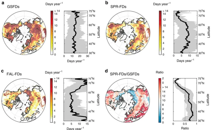
Spatial pattern of frost days during the past three decades.
Figure
1
shows the spatial distribution of the average number of
GSFDs in the Northern Hemisphere during 1982–2012. This
distribution is calculated using the 3-h Princeton and WFDEI
temperature data sets by counting the number of days with Tmin
< 0 °C during the growing season (average of both data sets, see
Methods). The largest numbers of GSFDs (>14 days per year) is
found in western North America, northeast Europe, Siberia, and
the Tibetan Plateau (Fig.
1
a). The number of frost days in spring
(SPR-FDs) vs. autumn (FAL-FDs) differs substantially among
regions. FAL-FDs are more frequent in northeastern Siberia and
the Tibetan Plateau (Fig.
1
c), and SPR-FDs in western North
America, northeastern Europe, and southeastern Siberia (Fig.
1
b).
The total number of GSFDs did not change with latitude (Fig.
1
a),
because the number of SPR-FDs (Fig.
1
b) and FAL-FDs (Fig.
1
c)
show changes in opposite direction with increasing latitude.
Figure
1
d displays the fraction of the total number of frost days
occurring in spring. The region south of 62 °N was mainly
affected by SPR-FDs, but Arctic regions were dominated by
FAL-FDs. Similar results were found using the middle day between
SOS and EOS, instead of the summer solstice (Fig.
1
), to separate
SPR-FDs and FAL-FDs, suggesting that such spatial pattern of
GSFDs at high latitudes was not due to a short spring (i.e., SOS
close to summer solstice, Supplementary Fig.
1
) (Supplementary
Fig.
2
a–d). The non-dominant role of SPR-FDs in GSFDs at high
latitudes is possibly because most (>80%) of SPR-FDs occurred
within a short time period (20 days) after the SOS
(Supplemen-tary Fig.
3
a,b). The Princeton and WFDEI Tmin
observations
provided consistent results (Supplementary Fig.
2
i-p), and also
the 6-h CRU-NCEP Tmin
observations indicated a similar, albeit
weaker (i.e., fewer in the number), spatial pattern of GSFDs,
probably because of its lower temporal resolution (Supplementary
Fig.
2
e–h).
Change in the number of growing season frost days. We next
examined the change in the number of GSFDs between the 1980s
and the 2000s. During this period, mean northern
growing-season temperatures (Tmin) increased by ~0.70 °C (0.75 °C in
spring, from SOS to summer solstice, 0.67 °C in autumn, from
summer solstice to EOS). Figure
2
a shows the spatial distribution
of changes in GSFDs. The number of GSFDs increased by more
than one day per year over more than 36% of the Northern
Hemisphere, mainly in Europe and central North America during
the last 30 years. The temporal distribution of these additional
GSFDs, however, differed between these two regions. The number
of GSFDs increased over ~82% of the area of Europe, and the
average increase in Europe was 2.8
± 4.6 extra frost days per
growing season (P
< 0.05, t-test) (Fig.
2
a). In Europe, increases
occurred mostly in spring (2.7
± 3.3 additional SPR-FDs per
growing season, P
< 0.05, t-test) (Fig.
2
d). In contrast, GSFDs
increased similarly in both spring and autumn in central North
America (Fig.
2
a, d, g). The increased SPR-FDs more likely
occurred during short periods (i.e., 43% within 10 days and 81%
within 1 month) after SOS (Supplementary Fig.
3
c–f). GSFDs
decreased in northern Siberia, the Tibetan Plateau, and
north-western North America (Fig.
2
a), mainly due to a decrease in the
number of FAL-FDs (Fig.
2
g). Overall, GSFDs decreased
sig-nificantly in about 34% of the Northern Hemisphere, which is
slightly lower than the area (~43%) that experienced a significant
increase (Fig.
2
a). The percentage of land areas where GSFDs
increased significantly was similar in autumn and spring (~40
versus ~45%) (Fig.
2
d, g). We derived similar results when using
the CRU-NCEP, Princeton, and WFDEI Tmin
data sets
indivi-dually (Supplementary Fig.
4
) instead of combining the Princeton
and WFDEI data sets (Fig.
2
).
Both growing season length (GSL) and temperature increased
between the 1980s and the 1990s and showed no significant
change between the 1990s and the 2000s
19–22. The 2000s is
marked by a warming hiatus in the Northern Hemisphere, with
decreasing temperature in spring over North America and winter
over Eurasia
23,24. We examined the effects of changing GSL and
Tmin
on GSFDs by analyzing the differences in the number of
GSFDs between the 1980s and the 1990s and between the 1990s
and the 2000s (Fig.
2
b, c). The GSFDs increased across more than
66% of the Northern Hemisphere area between the 1980s and the
1990s (significant over ~54%), but only over ~32% between the
1990s and the 2000s (significant over ~26%). The most
pronounced changes in GSFDs occurred in Eurasia, particularly
in Europe and central Siberia (Fig.
2
b, c), where the number of
GFSDs increased between the 1980s and the 1990s, and decreased
between the 1990s and the 2000s. The number of GSFDs
increased most (>4.0 additional frost days per growing season, P
< 0.05, t-test) in northern Europe between the 1980s and the
1990s and decreased most (>2.4 fewer frost days per growing
season, P
< 0.05, t-test) in central Siberia between the 1990s and
the 2000s (Fig.
2
b, c). These changes were more common in
spring than in autumn over the last 30 years (Fig.
2
), and the
changes in SPR-FDs nearly mirrored the changes in GSFDs.
Regions with consistent decreases in the number of GSFDs during
the periods 1980s-1990s and 1990s-2000s are northeastern Siberia
and consistent increases in southeastern Canada (Quebec, Sault
Ste. Marie, and Moosonee) (Fig.
2
b, c). This characterization of
changes in GSFDs between successive decades is rather insensitive
to the choice of the gridded temperature data sets (Supplementary
Fig.
4
) and meteorological station data (Supplementary Fig.
5
).
We also calculated the number of GSFDs in Europe using
in situ observations where leaf unfolding and leaf senescence were
defined as the start and end of growing season (European
phenology network, see Methods), and compared the results with
satellite-based estimates within the same periods (Fig.
2
and
Supplementary Fig.
6
). We found that the number of GSFDs
inferred from in situ records was always lower than those derived
from the satellite observations (Supplementary Fig.
6
), likely due
to the different spatial scales of the satellite (0.5° in this study)
and in situ (points) observations
25,26. Good correlations were
found between phenology data derived from GIMMS NDVI3g.v1
and MODIS EVI (SOS: R
= 0.93, P < 0.01, t-test; EOS: R = 0.59, P
< 0.01, t-test), suggesting the robustness of phenology-extraction
methods across different satellite data sets. Satellite-derived
phenology generally indicates a start of greening at a pixel scale,
which is dominated by the signal of the earliest species (often
ground cover), with EOS being dominated by the latest, and
typically different, species in the corresponding pixel
27,28. In
contrast, in situ phenological data are always derived from
individual trees, typically late-flushing species whose growing
season is much shorter than that of the entire spectrum of species
in the satellite image. Another possible reason was ascribed to the
fact that satellite derived SOS and EOS might not tightly relate to
the actual leaf unfolding and plant senescence
29,30. Despite the
difference in absolute numbers of GSFDs between in situ and
satellite-based calculations, the temporal pattern of GSFDs based
on in situ data is consistent with that of the satellite observations
in Europe (Fig.
2
and Supplementary Fig.
6
). The number of
in situ based GSFDs increased between the 1980s and the 1990s,
with averages of 0.6
± 0.9, 0.6 ± 1.0, and 0.3 ± 0.7 additional
GSFDs (991 sites), SPR-FDs (2655 sites) and FAL-FDs (1213 sites)
per year, respectively (P
< 0.05, t-test). The number of in situ
based GSFDs declined significantly between the 1990s and the
2000s, similar to the satellite-based GSFDs, by 0.5
± 1.0, 0.4 ± 1.0,
and 0.1
± 0.6 fewer GSFDs, SPR-FDs and FAL-FDs per year,
respectively (P
< 0.05, t-test) (Supplementary Fig.
6
a). We found
the same decadal changes of in situ GSFDs using other
gridded-temperature data sets, namely CRU-NCEP, Princeton and
WFDEI (Supplementary Fig.
6
b–d).
The contribution of phenology and temperature to GSFDs.
Changes in plant phenology (GSL) and in Tmin
can both influence
changes in GSFDs. To separate the contribution of these two
factors, we simulated the number of growing season frost days
based on our 30-yr observation record by (1) letting Tmin
change
according to temperature observations and keeping phenology
constant (scenario 1, see Methods for details), and (2) by letting
phenology change as in satellite observations but keeping Tmin
constant (scenario 2, see Methods for details). The comparison in
GSFDs between the two simulations and the actual estimates
allows us to separate the contribution of changes in GSL vs.
changes in Tmin. Changes in Tmin
alone lead us to observe a
decrease in the number of GSFDs between the 1980s and the
2000s across most of the Northern Hemisphere (Supplementary
Fig.
7
a). In contrast, the simulation with changes in GSL alone
produces an increase in the number of GSFDs (Supplementary
Fig.
7
b), by increasing the exposure of photosynthetically active
vegetation to periods when Tmin
< 0 °C. Overall, change in Tmin
was found to have a larger effect in reducing GSFDs across most
GSFDs SPR-FDs FAL-FDs SPR-FDs/GSFDs Ratio 0 2 4 6 8 10 12 14 > 14 0 10 20 30 75oN Latitude 0 2 4 6 8 10 12 14 > 14 0 5 10 15 Latitude 0 2 4 6 8 10 12 14 > 14 0 5 10 15 30oN 40oN 50oN 60oN 70oN 75oN Latitude 0 2 4 6 8 10 12 14 > 14 0 2 0 0.5 1 Ratio Latitude Days year–1 70oN 60oN 50oN 40oN 30oN 75oN 70oN 60oN 50oN 40oN 30oN 75oN 70oN 60oN 50oN 40oN 30oN
a
b
d
c
Days year–1 Days year–1 Days year–1 Days year–1 Days year–1Fig. 1 Spatial distribution of average frost days during growing season for 1982–2012. The number of frost days in the Northern Hemisphere was averaged from the results of the Princeton and WFDEI data sets.a–c indicates frost days and their variation along the gradient of latitude (black line and gray area presents the average frost days and its standard deviation across latitudes, respectively) calculated during growing season (GSFDs, from SOS to EOS), spring (SPR-FDs, from SOS to summer solstice) and autumn (FAL-FDs, from summer solstice to EOS).d displays the ratio of the number of frost days between (b) and (a). Maps were created using Matlab R2014b
of Asia and North America in 2000s compared to 1980s
(Sup-plementary Fig.
7
a and c). On the contrary, the extension of GSL
(primarily the advance of SOS) contributed more to the increase
in the number of GSFDs in Europe (Supplementary Figs.
7
c, e, f,
8
a, d). Besides the spatial discrepancies in factors regulating the
change in GSFDs, extended GSL was the dominant driving factor
determining the increasing GSFDs between the 1980s and the
1990s, opposite to the extensively reduced GSFDs due to changes
in Tmin
during the period 1990s and 2000s (Supplementary
Fig.
7
). This change in the driving factor of the GSFDs changes
between the
first two and the last two decades is mainly linked to
spring rather than to autumn (Supplementary Fig.
7
), probably
because the advancing trend in SOS between the 1980s and the
1990s stalled or even reversed between the 1990s and the
2000s
19,20. The same analysis based on three individual climatic
data sets also produced similar results (Supplementary Fig.
7
).
Evidence for the hypothesis. We further tested the hypothesis
that the number of GSFDs would increase as the growing season
gets longer by exploring the spatial relationship between satellite
derived phenological change and GSFDs in the Northern
Hemi-sphere at both continental (Fig.
3
and Supplementary Fig.
9
) and
local (Fig.
3
and Supplementary Fig.
10
) scales. At the continental
scale, the number of GSFDs generally increased more in regions
with faster extension of GSLs during all study periods (P
< 0.01,
t-sos-eos
a
FD2000–2009-FD1982–1989 sos-summer solsticed
Summer solstice-eosg
b
e
h
c
f
i
< –1.5 –1.5 –1 –0.5 0 0.5 1 1.5 > 1.5 Days year–1 FD1990–1999-FD1982–1989 FD2000–2009-FD1990–1999Fig. 2 Decadal changes in average frost days during growing season. The number of frost days (FD) in the Northern Hemisphere was averaged from the results of the Princeton and WFDEI data sets. The left, center, and right panels indicate the differences in the average number of frost days between the 1980s and the 2000s, the 1980s and the 1990s, and the 1990s and the 2000s. The upper, middle, and bottom panels show the time periods used to calculate the number of frost days (a–c GSFDs, from SOS to EOS, d–f SPR-FDs, from SOS to the summer solstice, and g–i FAL-FDs, from the summer solstice to EOS). Dotted areas indicate regions with significant changes (P < 0.05, t-test) in the number of frost days. Maps were created using Matlab R2014b
test), despite the warming (Fig.
3
a and Supplementary Fig.
9
a–c).
This association between increasing GSFDs and a longer GSL was
more apparent in spring (Fig.
3
b and Supplementary Fig.
9
d–f)
than autumn (Fig.
3
c and Supplementary Fig.
9
g-i). At the local
scale, the spatial partial correlation with a moving window of
2.5 × 2.5° also revealed that regions with longer GSL tended to
have more frost days during the growing season (Fig.
3
and
Supplementary Fig.
10
). More than 69% of the Northern
Hemi-sphere shows a significant positive partial correlation between
changes in GSL and changes in the number of GSFDs in each
decade, after statistically removing the effect of temperature
change (Fig.
3
d and Supplementary Fig.
10
a–c). This relationship
was much stronger than the partial correlation between the
changes in GSFDs and temperature (Fig.
3
g and Supplementary
Fig.
10
a–c), indicating that the phenological change influenced
the spatial pattern of changes in the occurrence of frost during
growing season at the local scale more than the change in
tem-perature. Analyses using the individual climatic data sets
sup-ported this result (Supplementary Figs.
9
and
10
).
Northern Hemisphere 47.8% 1.8% 17.2% 31.6% Change in GSFDs (days)
a
–20 –10 0 10 20 30 North America 40.8% 2.3% 30.2% 26.3% Europe 78.5% 0.7% 3.9% 16.5% Change in GSL (days) –30 –20 –10 0 10 20 30 –20 –10 0 10 20 30 Asia 41.2% 1.5% 14.1% 41.2% –30 –20 –10 0 10 20 30 Northern Hemisphere 2.9% 51.0% 25.6% 17.7% Change in SPR-FDs (days)b
–20 –10 0 10 20 30 North America 6.9% 38.3% 17.3% 36.3% Europe 1.0% 83.4% 12.6% 2.4%Change in SOS (days)
–30 –20 –10 0 10 20 30 –20 –10 0 10 20 30 Asia 0.8% 47.2% 36.3% 12.0% –30 –20 –10 0 10 20 30 Northern Hemisphere 41.6% 2.4% 20.9% 22.6%
Change in FAL-FDs (days)
c
–20 –10 0 10 20 30 North America 44.1% 2.1% 25.7% 23.8% Europe 55.0% 1.6% 9.9% 20.6%Change in EOS (days)
–30 –20 –10 0 10 20 30 –20 –10 0 10 20 30 Asia 36.6% 2.8% 22.1% 23.1% –30 –20 –10 0 10 20 30 0 0.1 0.2 0.3 0.4 0.5 0.6 0.7 0.8 0.9 > 0.9 Percentage (%)
d
Change in GSFDs-change in GSLg
Change in GSFDs-change in Tmine
Change in SPR-FDs-change in SOSh
Change in SPR-FDs-change in Tminf
Change in FAL-FDs-change in EOSi
Change in FAL-FDs-change in Tmin< –0.6 –0.6 –0.4 –0.2 0 0.2 0.4 0.6 > 0.6 Partial correlation coefficient
Fig. 3 Relationship between the changes in phenology and corresponding frost days. This relationship is presented between the 1980s and the 2000s at both continental and local scales. The number of frost days was averaged from the results of the Princeton and WFDEI data sets. The colors in the left panels (a–c heating plots with percentage of pixels in each quadrant, continental scale) indicate the proportions of pixels that fall within each binned area (i.e., every 1 day in the changes of the number of frost days and phenology) in the Northern Hemisphere. The center (d–f) and right (g–i) panels display the spatial partial correlations between changes in the number of frost days with phenology andTmin, respectively, using a moving window of 2.5 × 2.5° (i.e.,
Discussion
Our result shows that GSFDs increased mainly in Europe during
the last three decades, indicating an increase in the vegetation
exposure to cold events was found. However, it is still unclear
whether more frost days during the growing season would result
in more actual plant damage
31,32. The susceptibility of plant
growth to frost varies across species, and conditions
4,33, which
make it hard to directly compare the actual frost damage via
accounting the number of frost days during growing season.
Moreover, the susceptibility of plants to frost was found to
increase with the specific growth stage
34. Because the GSFDs are
not equally distributed during the growing season
(Supplemen-tary Fig.
3
a,b), the timing when the frost events occurred should
not be neglected when assessing the impact of frost on plants.
In this study, we used in situ phenological observations
(dis-tributed in Europe and only deciduous tree species) to
comple-ment the results based on satellite-derived phenology. Although
consistent changes in GSFDs were found, the large discrepancies
between in situ- and satellite- based phenology dates (due to
different spatial scales and inclusion of understory species in the
satellite images) as well as in the reported changes in GSFDs,
especially across other regions or species, should be investigated
and validated in future in situ and experimental studies.
More-over, GSFDs predominantly occurred in the short periods after
SOS and before EOS (Supplementary Fig.
3
a,b), suggesting that
the definition of SOS and EOS from NDVI data would impact the
quantification of GSFDs. Such concern, however, was less obvious
in estimating changes in GSFDs, because the result based on a
single method (i.e., Piecewise logistic method, Supplementary
Fig.
4
) produced a similar pattern as the result based on the mean
of four methods (Fig.
2
). Previous studies largely focused on both
in situ- and satellite- based spring phenology
15,28,35, but payed
less attention on autumn phenology
11,36. This likely originates
from the facts that autumn phenological events, such as leaf
senescence, cannot be as easily assessed by abrupt visual signals as
is the case for spring leaf out
30, and the mechanisms underlying
autumn phenology remain largely unknown
37. The periods used
for determining autumn frost days are less consistent as the
periods used for spring frost days. In addition, the susceptibility
of plant growth to frost during spring and autumn varies across
species, locations and different growth stages
4,33,34. Therefore,
in situ observations and
field experiments are urgently required to
improve the understanding of the linkage between autumn
phe-nology and autumn frost damage over the Northern Hemisphere.
In summary, the results of this study suggest that temperate
and boreal vegetation ecosystems have been experiencing
sig-nificant changes in the number of GSFDs. We found that the
number of GSFDs generally increased with the lengthening of the
growing season (especially in Europe and in spring) but decreased
in some regions due to global warming during the last three
decades. Moreover, GSFDs were less frequent in 2000s than
1990s, mainly because the SOS stopped advancing or even came
later in 2000s during the warming hiatus periods. The impact of
frost occurrence during growing season is likely species-specific
and also the carry-over effect might be different among species. It
was suggested that frost damage influences the timing of leaf-out
in temperate tree species
38and damages
flower buds and seeds of
montane wildflowers
3, reduces the gross productivity of forest
ecosystem
5and decreases the yield of economical crops
9. The
increase in frost occurrence during growing season could
mod-ulate the magnitude and even direction of the response of
regional vegetation growth to climate change
1,39,40and may offset
some of the benefits of a longer growing season, such as the
enhanced productivity in northern ecosystems. A longer growing
season may be a major mechanism for increasing productivity in
the Northern Hemisphere under global warming
41–44. Most
state-of-the-art models of the Earth ecosystem, however, do not take
into account the impacts of increasing growing season frost
occurrence on vegetation growth, implying that the ability of
northern ecosystems to sequester carbon may be overestimated.
Acquiring a better understanding of growing season frost
occurrence and its potentially damaging impact on vegetation
productivity is clearly a priority for developing strategies to
reduce the vulnerability of ecosystems under future climate
change.
Methods
Global climatic data sets. We extracted data for daily minimum temperature (Tmin) for calculating the number of GSFDs from three independent global climatic
data sets and one station-level data set from Global Surface Summary of the Day (GSOD). Three gridded data sets provided globally continuous records with a spatial resolution of 0.5 × 0.5°, but each was sampled with a different time interval for 1982 to 2012. First, CRU-NCEP v5 (CRU: Climatic Research Unit, NCEP: National Centers for Environmental Protection, hereafter CRU-NCEP, ftp://nacp. ornl.gov/synthesis/2009/frescati/model_driver/cru_ncep/analysis/readme.htm) is a 6-h data set based on the combination of records from globally distributed ter-restrial meteorological stations and NCEP reanalysis data45,46. Second, we used a
3-h sampled global data set produced by t3-he Terrestrial Hydrology Researc3-h Group at Princeton University47(hereafter Princeton, available fromhttp://hydrology. princeton.edu/data.pgf.php). This data set merges a reanalysis48with global
observations and is designed for modeling hydrological and land-surface processes. Temperature in this data set was corrected to match the Climatic Research Unit (CRU) time series (TS) v3.0 data set on a monthly scale before data publication46.
Last, we used the WFDEI meteorological forcing data set (WATCH Forcing Data methodology applied to ERA-Interim data,http://www.eu-watch.org/
data_availability), which uses data from an ERA-Interim reanalysis and provides Tminat time steps of 3 h49. All three data sets have been successfully applied in
recent studies of climate change47,50. GSOD data set was released by the National Climatic Data Center ( https://data.noaa.gov/dataset/global-surface-summary-of-the-day-gsod). We extracted 2626 stations with 31 years of available minimum temperature over the study period 1982–2012, and these stations were distributed across most of our study area.
Satellite-derived phenology. The seasonal variations of the Normalized Differ-ence Vegetation Index (NDVI), a proxy of vegetation greenness and photosynthetic activity51, is commonly used to interpret phenometrics (e.g., growing-season length (GSL), start of the growing season (SOS), and end of the growing season (EOS))52.
We derived the phenology in the Northern Hemisphere from the latest generation of NDVI records by NASA’s GIMMS group (GIMMS3g.V1, an updated from
pre-vious GIMMS3g). Errors and noise associated with the update of the satellite
sensors, atmospheric interference, and non-vegetation dynamics were addressed in GIMMS3g, while artifacts due to changes in calibration and replacement of negative
NDVI in snow-covered regions with zero values in previous version have been further processed53,54. We applied four widely used methods to extract phenology
dates: HANTS-Mr55, Polyfit-Mr56, Double logistic57and Piecewise logistic58. For
the HANTS-Mr and Polyfit-Mr methods, we fitted NDVI time-series via “har-monic analysis”55and“six-order polynomial function”56and determined the
phenology date with maximum increase/decrease in NDVI. For the Double logistic method, we used a double logistic function to smooth the NDVI data and the date of SOS/EOS was embedded in the formulation of this function (i.e., a model parameter)57. The Piecewise logistic method used pairs of sigmoid function tofit
the seasonal NDVI curve and defined the local maxima/minima for the derivatives offitted NDVI curve as SOS/EOS58. Wefirstly fitted the 24 bimonthly composited NDVI data averaged during 1982–2012 to remove the noise and then the day with maximum decrease in NDVI (differed in its definition in each method) during the second half of the year was identified as EOS59, while the day with maximum
increase in NDVI during thefirst half year was identified as SOS. Then, we used the NDVI of these dates as thresholds to estimate SOS and EOS in individual years. For pixels with two complete growing seasons, we used the start of thefirst growing season and end of the second growing season as the SOS and EOS of the entire year. However, for pixels with two growing seasons, but with the second growing season ending in the next year, we only took thefirst growing season into con-sideration. The combined mean from four methods was used for determining the growing season for each pixel at each year to minimize the uncertainty associated with their discrepancies in interpreting phenological information from the NDVI seasonal curve. Moreover, we compared NDVI-based phenology data with EVI-based phenology data to complement our analysis. Limited by the time span of MODIS EVI dataset (since 2000), we only compared the SOS/EOS dates over the period 2000–2009. To eliminate the spatial mismatch between these satellite data sets (i.e., 1/12 × 1/12° in GIMMS NDVI3g.v1and 0.05 × 0.05° in MODIS EVI), we
remapped the extracted phenology data into the same spatial resolution (0.5 × 0.5°).
In situ phenological data. In situ phenological data were downloaded from the PAN European Phenology network (project PEP725,http://www.pep725.eu/index. php), which offers open and unrestricted access to long-term phenological records from 26 European countries. The dates of leaf unfolding (i.e.,first visible leaf stalk) and leaf senescence (i.e., 50% of autumnal coloring) were inferred from the ancillary BBCH code (Biologische Bundesanstalt, Bundessortenamt und Chemische Industrie). To avoid potential bias due to outliers and insufficient observations, we did not use sites with leaf unfolding later than the end of June and leaf senescence earlier than the beginning of July and concentrated on sites with 28 years of observations of leaf unfolding (2655), leaf senescence (1213), and both (991) for 1982–2009.
Calculation of the number of frost days. Frost days were defined as days when Tminwas below freezing point of water (0 °C)17,18. We remapped the
satellite-derived phenological data (1/12° spatial resolution) to spatially match the spatial resolution of the climatic data set (Tmin, 0.5° spatial resolution). First, we calculated
the number of frost days during the growing season (GSFDs, from SOS to EOS) in the Northern Hemisphere for 1982–2012. We then divided our calculations into spring (SPR-FDs, from SOS to the summer solstice (i.e., 22 June in the Northern Hemisphere)) and autumn (FAL-FDs, from the summer solstice to EOS). We calculated the number of GSFDs under two scenarios to further distinguish between the effects of phenological and temperature trends on the change in the number of GSFDs in the Northern Hemisphere during the last three decades. In thefirst scenario, we only considered temperature changes and kept phenology constant (i.e., the phenological data were randomly selected for 1982–2012 and held constant). In the second scenario, we varied only phenology and used a constant temperature (i.e., temperature data were randomly selected for 1982–2012 and held constant). We randomly selected phenology or Tmin10 times for
1982–2012, applied them individually in the estimations, and used their averages to eliminate sampling bias. Due to the difference in temporal resolution, we presented the average number of GSFDs from the results of the 3-h Princeton and WFDEI data sets and listed the results inferred from the three individual data sets as alternative choices in the Supplementary Figs.2–10. We also calculated the GSFDs from in situ observed leaf unfolding to leaf senescence using three gridded climatic data sets, then separated them into SPR-FDs (from leaf unfolding to summer solstice) and FAL-FDs (from summer solstice to leaf senescence). Moreover, station-level GSOD minimum temperature was applied to replace gridded climatic data sets to complement our result. Finally, we also examined the robustness of using summer solstice as the cut-off point to separate GSFDs into SPR-FDs and FAL-FDs through two ways: (1) calculating the temporal distribution of SPR-FDs and FAL-FDs within each 10 days’ periods after SOS and before EOS, individually. (2) using the middle day between SOS and EOS to test whether the choice of summer solstice as the cut-off point of growing season would impact the con-tribution of SPR-FDs and FALL-FDs to GSFDs.
Data availability. The authors declare that the source data supporting thefindings of this study are provided with the paper.
Received: 2 April 2017 Accepted: 20 December 2017
References
1. Augspurger, C. K. Spring 2007 warmth and frost: phenology, damage and refoliation in a temperate deciduous forest. Funct. Ecol. 23, 1031–1039 (2009). 2. Beck, E. H., Fettig, S., Knake, C., Hartig, K. & Bhattarai, T. Specific and
unspecific responses of plants to cold and drought stress. J. Biosci. 32, 501–510 (2007).
3. Inouye, D. W. Effects of climate change on phenology, frost damage, andfloral abundance of montane wildflowers. Ecology 89, 353–362 (2008).
4. Snyder, R. L. & Melo-Abreu, J. P. in Frost Protection: Fundamentals, Practice and Economics. Volume 2 (FAO, 2005).
5. Hufkens, K. et al. Ecological impacts of a widespread frost event following early spring leaf‐out. Glob. Change Biol. 18, 2365–2377 (2012).
6. Martin, M., Gavazov, K., Koerner, C., Hättenschwiler, S. & Rixen, C. Reduced early growing season freezing resistance in alpine treeline plants under elevated atmospheric CO2. Glob. Change Biol. 16, 1057–1070 (2010).
7. Schreiber, S. G. et al. Frost hardiness vs. growth performance in trembling aspen: an experimental test of assisted migration. J. Appl. Ecol. 50, 939–949 (2013).
8. Estiarte, M. & Peñuelas, J. Alteration of the phenology of leaf senescence and fall in winter deciduous species by climate change: effects on nutrient proficiency. Glob. Change Biol. 21, 1005–1017 (2015).
9. Wolf, R. The Easter freeze of April 2007: a climatological perspective and assessment of impacts and services. (Technical Report 2008-01, NOAA/USDA, 2008).
10. Snyder, R. L. & Melo-Abreu, J. P. Frost protection: fundamentals, practice and economics. Frost Prot.: Fundam. Pract. Econ. 1, 1–240 (2005). Volume 1. 11. Gallinat, A. S., Primack, R. B. & Wagner, D. L. Autumn, the neglected season in
climate change research. Trends Ecol. Evol. 30, 169–176 (2015). 12. Ault, T. et al. The false spring of 2012, earliest in North American record.
Trans. Am. Geophys. Union 94, 181–182 (2013).
13. Cannell, M. G. J. in Crop Physiology of Forest Trees (eds Tigerstedt, P. M. A., Puttonen, P. & Koski, V.) (Helsinki University Press, Helsinki, 1985). 14. Kim, Y., Kimball, J. S., Didan, K. & Henebry, G. M. Response of vegetation
growth and productivity to spring climate indicators in the conterminous United States derived from satellite remote sensing data fusion. Agric. For. Meteorol. 194, 132–143 (2014).
15. Menzel, A. et al. European phenological response to climate change matches the warming pattern. Glob. Change Biol. 12, 1969–1976 (2006).
16. Linderholm, H. W. Growing season changes in the last century. Agric. For. Meteorol. 137, 1–14 (2006).
17. Easterling, D. R. Recent changes in frost days and the frost-free season in the United States. Bull. Am. Meteorol. Soc. 83, 1327–1332 (2002).
18. Meehl, G., Tebaldi, C. & Nychka, D. Changes in frost days in simulations of twentyfirst century climate. Clim. Dyn. 23, 495–511 (2004).
19. Jeong, S. J., Ho, C. H., Gim, H. J. & Brown, M. E. Phenology shifts at start vs. end of growing season in temperate vegetation over the Northern Hemisphere for the period 1982–2008. Glob. Change Biol. 17, 2385–2399 (2011). 20. Barichivich, J. et al. Large-scale variations in the vegetation growing season and
annual cycle of atmospheric CO2at high northern latitudes from 1950 to 2011.
Glob. Change Biol. 19, 3167–3183 (2013).
21. IPCC. The Physical Science Basis: Contribution of Working Group I to the Fifth Assessment Report of the Intergovernmental Panel on Climate Change. (Cambridge University Press, 2013).
22. Piao, S., Fang, J., Zhou, L., Ciais, P. & Zhu, B. Variations in satellite-derived phenology in China’s temperate vegetation. Glob. Change Biol. 12, 672–685 (2006).
23. Cohen, J. L., Furtado, J. C., Barlow, M., Alexeev, V. A. & Cherry, J. E. Asymmetric seasonal temperature trends. Geophys. Res. Lett. 39, L04705 (2012).
24. Li, C., Stevens, B. & Marotzke, J. Eurasian winter cooling in the warming hiatus of 1998–2012. Geophys. Res. Lett. 42, 8131–8139 (2015).
25. Doktor, D., Bondeau, A., Koslowski, D. & Badeck, F.-W. Influence of heterogeneous landscapes on computed green-up dates based on daily AVHRR NDVI observations. Remote Sens. Environ. 113, 2618–2632 (2009).
26. Rodriguez-Galiano, V. F., Dash, J. & Atkinson, P. M. Intercomparison of satellite sensor land surface phenology and ground phenology in Europe. Geophys. Res. Lett. 42, 2253–2260 (2015).
27. Vrieling, A. et al. Spatially detailed retrievals of spring phenology from single-season high-resolution image time series. Int. J. Appl. Earth Obs. Geoinf. 59, 19–30 (2017).
28. Fu, Y. H. et al. Recent spring phenology shifts in western Central Europe based on multiscale observations. Glob. Ecol. Biogeogr. 23, 1255–1263 (2014). 29. White, M. A. et al. Intercomparison, interpretation, and assessment of spring
phenology in North America estimated from remote sensing for 1982–2006. Glob. Change Biol. 15, 2335–2359 (2009).
30. Tang, J. et al. Emerging opportunities and challenges in phenology: a review. Ecosphere 7, e01436 (2016).
31. Schwartz, M. D. Assessing the onset of spring: a climatological perspective. Phys. Geogr. 14, 536–550 (1993).
32. Schwartz, M. D., Ahas, R. & Aasa, A. Onset of spring starting earlier across the Northern Hemisphere. Glob. Change Biol. 12, 343–351 (2006).
33. Augspurger, C. K. Reconstructing patterns of temperature, phenology, and frost damage over 124 years: spring damage risk is increasing. Ecology 94, 41–50 (2013).
34. Lenz, A., Hoch, G., Vitasse, Y. & Körner, C. European deciduous trees exhibit similar safety margins against damage by spring freeze events along elevational gradients. New Phytol. 200, 1166–1175 (2013).
35. Wang, X. et al. Has the advancing onset of spring vegetation green‐up slowed down or changed abruptly over the last three decades? Glob. Ecol. Biogeogr. 24, 621–631 (2015).
36. Liu, Q. et al. Temperature, precipitation, and insolation effects on autumn vegetation phenology in temperate China. Glob. Change Biol. 22, 644–656 (2016).
37. Körner, C. et al. Where, why and how? Explaining the low‐temperature range limits of temperate tree species. J. Ecol. 104, 1076–1088 (2016).
38. Lenz, A., Hoch, G., Körner, C. & Vitasse, Y. Convergence of leaf‐out towards minimum risk of freezing damage in temperate trees. Funct. Ecol. 30, 1480–1490 (2016).
39. Gu, L. et al. The2007 Eastern US spring freeze: increased cold damage in a warming world? Bioscience 58, 253–262 (2008).
40. Fracheboud, Y. et al. The control of autumn senescence in European aspen. Plant. Physiol. 149, 1982–1991 (2009).
41. Keeling, C. D., Chin, J. & Whorf, T. Increased activity of northern vegetation inferred from atmospheric CO2measurements. Nature 382, 146–149 (1996).
42. Richardson, A. D. et al. Influence of spring and autumn phenological transitions on forest ecosystem productivity. Philos. Trans. R. Soc. Lond. B. Biol. Sci. 365, 3227–3246 (2010).
43. Piao, S., Friedlingstein, P., Ciais, P., Viovy, N. & Demarty, J. Growing season extension and its impact on terrestrial carbon cycle in the Northern Hemisphere over the past 2 decades. Global Biogeochemical Cycles 21,https:// doi.org/10.1029/2006GB002888(2007).
44. Keenan, T. F. et al. Net carbon uptake has increased through warming-induced changes in temperate forest phenology. Nat. Clim. Change 4, 598–604 (2014).
45. New, M., Hulme, M. & Jones, P. Representing twentieth-century space-time climate variability. Part II: development of 1901–96 monthly grids of terrestrial surface climate. J. Clim. 13, 2217–2238 (2000).
46. Mitchell, T. D. & Jones, P. D. An improved method of constructing a database of monthly climate observations and associated high-resolution grids. Int. J. Climatol. 25, 693–712 (2005).
47. Sheffield, J., Goteti, G. & Wood, E. F. Development of a 50-year high-resolution global dataset of meteorological forcings for land surface modeling. J. Clim. 19, 3088–3111 (2006).
48. Kalnay, E. et al. The NCEP/NCAR 40-year reanalysis project. Bull. Am. Meteorol. Soc. 77, 437–471 (1996).
49. Weedon, G. P. et al. The WFDEI meteorological forcing data set: WATCH Forcing Data methodology applied to ERA‐Interim reanalysis data. Water Resour. Res. 50, 7505–7514 (2014).
50. Naudts, K. et al. Europe’s forest management did not mitigate climate warming. Science 351, 597–600 (2016).
51. Myneni, R. B., Hall, F. G., Sellers, P. J. & Marshak, A. L. The interpretation of spectral vegetation indices. IEEE Trans. Geosci. Remote Sens. 33, 481–486 (1995).
52. Buitenwerf, R., Rose, L. & Higgins, S. I. Three decades of multi-dimensional change in global leaf phenology. Nat. Clim. Change 5, 364–368 (2015). 53. Tucker, C. J. et al. An extended AVHRR 8‐km NDVI dataset compatible with
MODIS and SPOT vegetation NDVI data. Int. J. Remote. Sens. 26, 4485–4498 (2005).
54. Pinzon, J. E. & Tucker, C. J. A non-stationary 1981–2012 AVHRR NDVI3g time series. Remote Sens. 6, 6929–6960 (2014).
55. Jakubauskas, M. E., Legates, D. R. & Kastens, J. H. Harmonic analysis of time-series AVHRR NDVI data. Photogramm. Eng. Remote Sens. 67, 461–470 (2001).
56. Piao, S. et al. Leaf onset in the northern hemisphere triggered by daytime temperature. Nat. Commun. 6, 6911 (2015).
57. Julien, Y. & Sobrino, J. Global land surface phenology trends from GIMMS database. Int. J. Remote. Sens. 30, 3495–3513 (2009).
58. Zhang, X. et al. Monitoring vegetation phenology using MODIS. Remote Sens. Environ. 84, 471–475 (2003).
59. Liu, Q. et al. Delayed autumn phenology in the Northern Hemisphere is related to change in both climate and spring phenology. Glob. Change Biol. 22, 3702–3711 (2016).
Acknowledgements
This study was supported by the National Natural Science Foundation of China (41530528), the National Key R&D Program of China (2017YFA0604702), the 111 Project (B14001), and National Youth Top-notch Talent Support Program in China. Philippe Ciais, Ivan A Janssens and Josep Peñuelas acknowledge support from the European Research Council through Synergy grant ERC-2013-SyG-610028 “IMBAL-ANCE-P”.
Author contributions
S.P. designed the research; Q.L. performed the analysis; S.P. and Q.L. drafted the paper; and S.P., Q.L., I.A.J., Y.F., S.P, X.L., P.C., R.B.M., J.P. and T.W. contributed to the interpretation of the results and to the text.
Additional information
Supplementary Informationaccompanies this paper at https://doi.org/10.1038/s41467-017-02690-y.
Competing interests:The authors declare no competingfinancial interests. Reprints and permissioninformation is available online athttp://npg.nature.com/ reprintsandpermissions/
Publisher's note:Springer Nature remains neutral with regard to jurisdictional claims in published maps and institutional affiliations.
Open Access This article is licensed under a Creative Commons Attribution 4.0 International License, which permits use, sharing, adaptation, distribution and reproduction in any medium or format, as long as you give appropriate credit to the original author(s) and the source, provide a link to the Creative Commons license, and indicate if changes were made. The images or other third party material in this article are included in the article’s Creative Commons license, unless indicated otherwise in a credit line to the material. If material is not included in the article’s Creative Commons license and your intended use is not permitted by statutory regulation or exceeds the permitted use, you will need to obtain permission directly from the copyright holder. To view a copy of this license, visithttp://creativecommons.org/ licenses/by/4.0/.
© The Author(s) 2018