Bootstrapping a Hedonic Price Index: Experience from Used Cars Data

Texte intégral

(1)Paper published in AStA Advances in Statistical Analysis, DOI 10.1007/s10182-006-0015-9. The original publication is available at www.springerlink.com.. Bootstrapping a Hedonic Price Index: Experience from Used Cars Data Michael Beer∗ January 20, 2007.. Abstract Every hedonic price index is an estimate of an unknown economic parameter. It depends, in practice, on one or more random samples of prices and characteristics of a certain good. Bootstrap resampling methods provide a tool for quantifying sampling errors. Following some general reflections on hedonic elementary price indices, this paper proposes a case-based, a model-based, and a wild bootstrap approach for estimating confidence intervals for hedonic price indices. Empirical results are obtained for a data set on used cars in Switzerland. A simple and an enhanced adaptive semi-logarithmic model are fit to monthly samples, and bootstrap confidence intervals are estimated for Jevons-type hedonic elementary price indices. Key words: hedonic regression, hedonic price indices, bootstrap methods, wild bootstrap, confidence intervals, used cars. JEL classification: C43, C15, E31, L62.. 1 Introduction One of the most difficult problems in the estimation of a consumer price index (CPI) is the handling of quality changes. The hedonic approach provides one possible manner of tackling this problem. Its main idea is to identify the quality of a product—or, in other words, its ‘potential contribution . . . to the welfare and happiness of its purchasers and the community’ (Court, 1939, p. 107)—with a vector of product characteristics. A regression equation is then estimated relating the latter to the price of the product. This allows, with regard to price index estimation, to control for quality differences over time and to impute prices for product variants that are, for instance, no longer available for price observation. In this sense, the hedonic index approach can be seen as the ‘most intellectually satisfying of the various quality-adjustment methods because ∗. The author was a research assistant and PhD candidate at the Seminar of Statistics, Department of Quantitative Economics, University of Freiburg/Fribourg Switzerland, Bd. de Pérolles 90, CH-1700 Freiburg (e-mail: research@michael.beer.name). This study is part of the project entitled ‘Specification, axiomatic foundation, and estimation of hedonic price indices’ funded by the Swiss National Science Foundation as well as the Swiss Federal Statistical Office and directed by Hans Wolfgang Brachinger. Thanks are owed to him for his most appreciated comments on preliminary versions of this paper, to João Santos Silva for proposing the wild bootstrap approach, to an anonymous referee for advocating the advantages of the enhanced modelling approach and to the audience at the ‘Statistische Woche 2005’ in Braunschweig for their contributions.. 1.

(2) it appeals to an underlying economic structure rather than to opportunistic proxies’ (Hulten, 2003, p. 9). In practice, the relationship between characteristics and price of a certain good has to be estimated on the basis of a sample of market observations. Therefore, every hedonic price index has to be viewed as a random variable. Yet, there are statistical methods that allow the quantification of its degree of randomness. In the present paper, the estimation of confidence intervals for hedonic price indices using bootstrap samples is investigated. It formalises and extends thus the idea of Pakes (2003), who used bootstrap techniques to estimate standard errors of hedonic price index estimates. This article starts with a methodical introduction to hedonic indices. A stochastic model for hedonic regressions is established, and the hurdles to overcome in order to estimate a hedonic index are briefly discussed. Section 3 presents three methods for generating bootstrap replications of hedonic function estimates which can be used for quantifying the estimation error of hedonic price indices. These methods are finally applied to a novel data set on used cars in Switzerland.. 2 Hedonic Functions and Hedonic Indices 2.1 From the hedonic hypothesis to the hedonic price index The estimation of a CPI normally proceeds in two stages. First, elementary price indices are estimated for every single good or, more precisely, for every elementary expenditure aggregate of a CPI. Secondly, these elementary indices are aggregated to higher-level indices using the expenditure shares of these aggregates as weights. An elementary aggregate, in this context, consists of ‘a small and relatively homogeneous set of products defined within the consumption classification used in the CPI’. Frequently, elementary aggregates are the lowest level at which any reliable expenditure information is available. This is the reason why, ‘In most cases, the price indices for elementary aggregates are calculated without the use of explicit expenditure weights’ (ILO et al., 2004, pp. 14ff). Quality adjustment is generally an issue that plays its role on this elementary aggregate level rather than for the estimation of higher-level price indices. Most of the hedonic indices are therefore by nature elementary price indices. They start from the idea that the quality of a given good can be identified with a vector of its characteristics, and that the price of a good can be explained as a function of its quality. More precisely, it is assumed that, for every variant of a good, the equation pt = ht (m) + ǫt (1) holds, where pt is the price of the variant at time t, m is a K-dimensional vector of price-relevant characteristics, ǫt is a quality-independent price residual and ht is the so-called hedonic function. This assumption is called the hedonic hypothesis. Due to changing market conditions, one and the same quality may not be attributed the same price at different points in time. The discrepancy between the hedonic functions at two separate time periods can thus be interpreted as a quality-adjusted measure of inflation. In other words, if the characteristics vector m is fixed, the ratio h1 (m)/h0 (m) represents the price change between a base period 0 and a reference period 1 of the quality represented by m. A hedonic elementary price index is an average of such price ratios over the whole quality spectrum of a good, where, in practice, this quality spectrum is represented by a fixed list of N characteristics vectors m1 , . . . , mN .. 2.

(3) The question of how to choose these N quality vectors is important. One possible approach might be to determine these reference qualities explicitly by choosing a set of representative variants of the good. Such an approach reflects the practice of statistical offices in price index estimation, where, usually, a pre-defined set of variants of a good is observed over time. This strategy starts from the idea that the representative variants are determined by a market survey of the most commonly bought products. In this case, however, the individual variants, or qualities, need to be weighted according to their sales or expenditure volumes in order to reflect their different market shares. Alternatively, one could build the reference list m1 , . . . , mN using elements of the database which, in any case, needs to be assembled for estimating the hedonic functions. This data generally covers an extensive spectrum of variants and builds thus a representative sample of the transactions for a certain good in a specific market over a certain time period. In this approach, a weighting as described in the previous paragraph might not be necessary. If frequently sold items appear as frequently in this database and thus also in the list of representative variants, an implicit weighting according to sales volumes is automatically carried out. Once the vectors m1 , . . . , mN are chosen, virtually all of the traditional elementary index formulae can be used to average the price relatives mentioned above. In the following analysis, the Jevons formula v uN u Y h1 (mn ) N 0:1 IJ = t (2) h0 (mn ) n=1. will be used as the model elementary index. Large theoretical support for this formula can be found in the literature (see ILO et al., 2004, Chap. 20). Empirical support for its application in a hedonic price index framework is provided, for instance, by Yu (2003).. 2.2 Estimating the hedonic function The estimation of the hedonic function ht at a specific point t in time is fundamental for the subsequent estimation of a hedonic elementary price index. For a randomly chosen variant of a good, at time t, its K-dimensional vector of price-relevant characteristics will be regarded as random vector denoted by M t , while the random variable P t stands for the price of this variant. The hedonic hypothesis leads then to an individual regression model P t = ht (M t ) + ǫt. (3). for each period t under consideration with the usual assumption that Eǫt = 0 for all t. For the beginning, no additional assumption is made on the variance structure of ǫt . The starting point for the estimation of the hedonic function is always a sample of different representatives of the good in question at time t. More specifically, the estimation of ht is based on a random sample of N t i.i.d. realisations (P1t , M t1 ), . . . , (PNt t , M tN t ) ,. (4). L where (Pnt , M tn ) ∼ (P t , M t ) for all n ∈ {1, . . . , N t }. K If H := {h : R −→ R≥0 } denotes the admissible hedonic functions applicable to the given ˆ t of the hedonic function ht results then from a mapping good, any estimate h t. t. N ×K h : RN ≥0 × R t (P , Mt ). −→ H ˆ t := h[P t , Mt ] 7−→ h. 3. (5).

(4) where P t = (P1t , . . . , PNt t ) denotes the random vector of sampled prices and Mt is the respective ˆt N t × K random matrix (M t1 , . . . , M tN t ) of the price-relevant characteristics.1 It follows that h is actually a random variable with values in H. ˆ t as an estimator (i.e. In order to simplify the notation, no distinction will be made between h a random variable with values in H) or as an estimation (i.e. an element of H) of ht . It should be clear from the context, which of the two meanings is applicable. Given any specific variant of the good with characteristics vector m, its price predictor is then defined by ˆ t (m) = h[P t , Mt ](m) . Pˆ t := h (6) In this case, the vector m is not random but fixed in advance. The randomness of Pˆ t stems ˆt. from the randomness of the estimator h. 2.3 Estimating the hedonic price index ˆ 0 and h ˆ 1 of the hedonic functions as well as a list of reference quality Given the estimations h vectors m1 , . . . , mN , the hedonic price index (2) can be estimated straightforwardly by v uN uY h ˆ 1 (mn ) N 0:1 ˆ IJ = t . (7) ˆ0 n=1 h (mn ). It is important to note that the reference quality vectors may or may not stem from the data ˆ 0 and h ˆ 1 respectively. Whether or not this is the case M0 and M1 used to get the estimations h depends on the specification of the hedonic index as discussed in Sect. 2.1. The formula (7) pretends that only imputed (estimated) prices are used in the calculations even though observed prices might be available for certain characteristics vectors mn in one or the other time period. It resembles the double imputation method as outlined in detail by Triplett (2004, pp. 70ff) and used in the analysis of Yu (2003). It would thus be in conflict with the practice of most hedonic index studies, where prices are imputed only for variants entering or exiting the market during the considered time period, whereas observed prices are used wherever possible. ˆ t is defined such that the observed price One could, however, imagine, that the estimator h t p of a specific variant at time t is taken as an estimate of ht (mn ) if mn corresponds to the characteristics vector of this variant. This is particularly relevant if the reference vectors mn are effectively taken from the database used for the estimation of the hedonic functions, because in this case, an observed price is available for every mn for at least one of the two time periods, ˆ t would mean that double imputation albeit not necessarily for the period t. This choice of h only takes place if, for a given mn , neither the base period price nor the current period price is available. The question of whether or not double imputation is admissible, has been discussed with scepticism by Triplett (2004, p. 70ff). He concludes that this matter ‘is not settled, and depends . . . on one’s interpretation of hedonic residuals’. Pakes (2003, p. 1589) empirically compares resulting index values under one and the other regime and discovers that they are ‘virtually identical’. One argument at least that could speak for discarding the observed prices is that ǫt actually represents the quality-independent price component as described in Sect. 2.1. If the hedonic 1. To simplify the notation, the transposed sign ‘′ ’ will generally be omitted when writing vectors and matrices within the text.. 4.

(5) function is correctly specified, the exclusive use of imputed prices would thus allow to get rid of these unsystematic price components.. 3 Bootstrap Replications of Hedonic Price Indices 3.1 Estimation error and confidence intervals The index formula given in (7) is a point estimator for the respective hedonic elementary price ˆ 0 and h ˆ 1 are random in nature, this ranindex (2). Given that the hedonic price predictors h 0:1 domness propagates to the estimator IˆJ . Trying to deduce the probability distribution of IˆJ0:1 analytically from those of its constituents seems ambitious given the potential complexity of the hedonic functions. Yet, it is possible to employ Monte-Carlo simulations to estimate its distribution empirically. Let us define the random estimation error of the Jevons-type hedonic elementary price index estimator IˆJ0:1 for a given list of reference characteristics m1 , . . . , mN by v v uN uN uY h u Y h1 (mn ) 1 ˆ (mn ) N N 0:1 0:1 0:1 t ˆ . (8) ζ := IJ − IJ = − t ˆ 0 (mn ) h0 (mn ) h n=1. n=1. A sensible method for qualifying the estimator IˆJ0:1 is the estimation of confidence intervals. An equitailed (1 − 2α) confidence interval for IJ0:1 is given by h i 0:1 ˆ0:1 IˆJ0:1 − ζ1−α , IJ − ζα0:1 (9). 0:1 are the α and (1 − α) quantiles of ζ 0:1 respectively. where ζαt and ζ1−α In order to determine these quantiles, some knowledge on the probability distribution of ζ 0:1 is needed. Bootstrap resampling methods, as they are extensively described, e.g., by Davison and Hinkley (1997), provide one manner of acquiring such knowledge. Their main idea is to use computer simulations for generating an empirical approximation of the distribution of interest based on new arrangements of the input data. These arrangements are essentially random samples drawn with replacement from the original data set. In this sense, the distribution of ζ 0:1 may be estimated by the distribution of v v uN uN uY h uY h 1 (m ) ˆ ˆ 1 (mn ) n N N ⋆ 0:1 t ζ⋆ := − t . (10) ˆ 0 (mn ) ˆ 0 (mn ) h h n=1. ⋆. n=1. ˆ 0 and h ˆ 1 are bootstrap replications of the hedonic price predictors, while h ˆ0, h ˆ 1 and the Hereby, h ⋆ ⋆ vectors m1 , . . . , mN remain fixed. The following section is going to discuss how such replications can be acquired.. 3.2 Resampling methods A first and most generally applicable bootstrap approach is the so-called case-based resampling procedure (see Davison and Hinkley, 1997, Sect. 6.2.4). For both periods t ∈ {0, 1}, a sample of N t price-characteristics combinations is drawn with replacement from the N t original data points at period t. This new sample is then used as an input to the regression algorithm h from ˆ 1 are obtained. Repeating this procedure R times leads to ˆ 0 and h where simulated values of h ⋆ ⋆ R new estimates of the hedonic function in both time periods, from where R replications of ζ⋆0:1 can be deduced.. 5.

(6) Algorithm 3.1 (Case-based resampling). For r = 1, . . . , R, for t ∈ {0, 1}, t , . . . , νt t 1. sample ν⋆1 ⋆N t randomly with replacement from {1, . . . , N }. 2. for n = 1, . . . , N t , set pt⋆n = ptν t and mt⋆n = mtν t ; ⋆n. ⋆n. ˆ t := h[pt , Mt ], where pt = (pt , . . . , pt t ) and Mt = (mt , . . . , mt t ). 3. compute h ⋆r ⋆ ⋆ ⋆ ⋆ ⋆1 ⋆1 ⋆N ⋆N. ⋄. It is such a case-based bootstrap procedure that Pakes (2003) apparently used for the estimation of standard errors of hedonic elementary price indices for PCs. A second approach is the model-based resampling, where the resampling takes place on the residuals of the original model (see Davison and Hinkley, 1997, Sect. 6.2.3). The underlying idea here is that, given the model (3), the regression residuals are estimates of the random errors ǫt . A simulated price for a certain characteristics vector mtn can thus be obtained by adding such ˆ t (mt ). a residual to the regression fit h n An important condition of the model-based approach is that the residuals involved need to be suitable for simulating the distribution of the random errors ǫt . In other words, the raw residuals ˆ t (mt ) need in general to be modified such that they have the same variance as ǫt etn = ptn − h n before they can be used for a model-based resampling. In the case of linear regression, i.e. if (3) is specified by P t = Xt β t + ǫt where Xt is the design matrix containing the data Mt plus a constant, the vector of raw residuals et = (et1 , . . . , etN t ) can be written as et = (I − Ht )ǫt where Ht = Xt (Xt′ Xt )−1 Xt′ is the hat matrix of the regression model at time t. Therefore, Davison and Hinkley (1997, p. 261) recommend to work with the modified residuals rnt =. ˆ t (mt ) ptn − h n (1 − htn )1/2. (11). where htn is the nth diagonal element of Ht , because their variances agree with those of ǫt . This makes sense if the standard assumption of homoscedasticity of the ǫt is tenable. In order to get proper estimates of ǫt having mean zero, the values of rnt are finally going to be re-centered by individually subtracting their average r¯t . Algorithm 3.2 (Model-based resampling). For r = 1, . . . , R, 1. for t ∈ {0, 1}, for n = 1, . . . , N t , t −r a) sample ǫt⋆n from r1t − r¯t , . . . , rN ¯t ; t. ˆ t (mt ) + ǫt ; b) compute the simulated response pt⋆rn = h n ⋆n ˆ t := h[pt , Mt ], where pt = (pt , . . . , pt t ). 2. compute h ⋆r ⋆r ⋆r ⋆r1 ⋆rN. ⋄. The inconvenience of the model-based resampling is the fact that properly modified, i.e. variance-adjusted residuals may not be easy to acquire, especially when the regression approach h is, e.g., non-linear. In such regression models, the so-called leverages htn are not available straight away. Moreover, the assumption of homoscedasticity of the random errors ǫt may not be justified. This is particularly true if one assumes that the model residuals ǫt are not just random noise but economically significant. (See Reis and Santos Silva, 2002 or Triplett, 2004, p. 186ff for some comments on the issue of heteroscedastic error terms in hedonic regressions.). 6.

(7) Case-based resampling, in contrast, is always applicable and does not depend on any assumption about ǫt . Yet, Davison and Hinkley (1997, p. 264ff) identify two disadvantages of casebased compared to model-based resampling. First, they state that case-based estimations might be inefficient if the constant-variance model is correct, and, secondly, they argue that case-based simulations lead to simulated samples with different designs, because the vectors mt⋆1 , . . . , mt⋆N t are randomly sampled. The design matrix of a regression model, however, ‘fixes the information content of a sample, and in principle our inference should be specific to the information in our data’. A third approach which overcomes the disability of the model-based approach to cope with heteroscedastic error terms is the so-called wild bootstrap originally proposed by Liu (1988) and developed further by Davidson and Flachaire (2001). Here, the error terms ǫt1 , . . . , ǫtN t are still assumed to be mutually independent and to have a common mean of zero, but they may be heteroscedastic with E[(ǫtn )2 ] = (σnt )2 . The error term, in this case, may be written as ǫtn = σnt vnt where E[vnt ] = 0 and E[(vnt )2 ] = 1. Correspondingly, the simulated prices pt⋆rn are ˆ t (mt ) any ǫt sampled from the centered modified residuals, no longer obtained by adding to h n ⋆n but by adding the corresponding modified residual (11) multiplied by a random number ǫt⋆n drawn from a completely independent auxiliary distribution having mean zero and variance one. For the case of hypothesis testing, both Davidson and Flachaire (2001) and MacKinnon (2002) advise to draw the numbers ǫt⋆n from the Rademacher distribution, i.e. from a discrete random variable having either the value −1 or 1 with probability 1/2 each. For the estimation of confidence intervals, there is weaker evidence for this specific choice and other alternatives such as the one proposed by Mammen (1993) might also be appropriate. This topic needs further research. Nevertheless, the Rademacher distribution is going to be proposed in the following third resampling approach. Algorithm 3.3 (Wild bootstrap). For r = 1, . . . , R, 1. for t ∈ {0, 1}, for n = 1, . . . , N t , a) sample ǫt⋆rn from a discrete random variable having either the value −1 or 1 with probability 1/2 each; ˆ t (mt ) + r t ǫt ; b) compute the simulated response pt⋆rn = h n n ⋆rn ˆ t := h[pt , Mt ], where pt = (pt , . . . , pt t ). 2. compute h ⋆r ⋆r ⋆r ⋆r1 ⋆rN. ⋄. The main advantage of the wild bootstrap compared to the model-based approach is its ability to incorporate heteroscedastic error terms. Moreover, it shares the property of the model-based approach concerning the unmodified regression design. However, it is an open question whether its efficiency is still better than the one of the case-based approach. ˆ 1 , a sample of simulated Regardless of the approach that is chosen for the simulation of ˆ h0⋆ and h ⋆ 0:1 , . . . , ζ 0:1 is finally calculated by (10). Furthermore, if the increasingly estimation errors ζ⋆1 ⋆R 0:1 (r = 1, . . . , R) are denoted by ζ 0:1 , . . . , ζ 0:1 , an estimate of the confidence ordered values of ζ⋆r ⋆[1] ⋆[R] interval (9) is given by h i 0:1 0:1 IˆJ0:1 − ζ⋆[(R+1)(1−α)] . (12) , IˆJ0:1 − ζ⋆[(R+1)α]. For this reason, the number R of bootstrap replications has to be chosen such that (R + 1)α is an integer. It should be noted that, at this stage, the regression approach h remains completely unspecified. Moreover, these resampling approaches do not depend on the specification of the hedonic price index by the Jevons formula. They are similarly applicable to any other index formula as well.. 7.

(8) 4 Hedonic Price Indices and Bootstrap Confidence Intervals for Used Cars in Switzerland 4.1 The data The empirical data used in this study stems from AutoScout24 AG, a private company maintaining an internet platform for selling cars. Their database consists of constantly around 70 000 advertisements of new or used cars that individuals or institutional dealers from all around Switzerland are offering. Along with the requested price, a series of characteristics is given for each car. Among these are the make and model name, the body type, the exterior and interior colour, the fuel type, the number of doors, seats, and cylinders as well as the cubic capacity and the horsepower of the engine. Moreover, there is the date of first registration—from where the age in months at placement time of the advertisement is calculated—, the current mileage, sometimes the original price and information on the remaining warranty in months and whether or not this car has been involved in an accident. Apart from that, there are over thirty equipment dummies (airbag, air conditioning, leather seats, sliding roof, etc.). This data has been available on a daily basis as of October 20, 2004. For the current analysis, only advertisements for the category of ‘used cars’ have been considered, throwing away all cars marked as ‘new’, ‘demonstration car’ or ‘oldtimer’. Moreover, advertisements where the price or the year of first registration were missing have been discarded as well. The huge number of observations available in this database along with the highly standardised characteristics variables make it attractive for a hedonic study. Its main fault, however, is the fact that only offering prices are provided which potentially differ significantly from the factual transaction prices. Moreover, the individual data points display the universe of offered and not of effectively bought cars. Great care is thus needed when interpreting the numerical results of this study. In other words, the results provided here are only numerically tenable under the assumptions that, firstly, the cars are sold at the same price as they are offered and, secondly, that the range of supplied cars is representative to the range of cars factually sold, and not only offered, in a certain time period. Since our prevalent aim, however, is the exploration of methods rather than the interpretation of the resulting index values, this drawback is going to be ignored for the moment. All the estimations were done using the R software for statistical computing (see R Development Core Team, 2006).. 4.2 Estimating the hedonic functions 4.2.1 The simple semi-logarithmic approach For the hedonic regressions, as a first approach, a semi-logarithmic functional form has been chosen relating the log of the price to a linear combination of the characteristics variables. In other words, the hedonic function has been specified by the model t. ln P =. β0t. +. K X. βkt Mkt + η t. (13). k=1. leading to a price predictor of the form ˆt. t. t. h (m) = h[P , M ](m) = exp. βˆ0t [P t , Mt ]. +. K X k=1. 8. βˆkt [P t , Mt ]mk. !. (14).

(9) where βˆkt [P t , Mt ] (k = 0, . . . , K) are the OLS parameter estimates given the training data set for period t. The error term, herein, is denoted by η t in order to distinguish it from ǫt in (3). This semi-logarithmic approach is perfectly in line with numerous other studies on hedonic price indices. According to Murray and Sarantis (1999, p. 9), ‘almost all studies of automobiles’ have followed this practice. This even holds for the model proposed by Court (1939, p. 110) in one of the very first articles on hedonic indices. Such a dominance of the semi-logarithmic functional form over all the others for this kind of study is due to the fact that very often, this approach better fitted the data than any similarly simple alternative. For the current study, additionally, an automated variable selection procedure2 based on the Akaike information criterion (AIC) was independently applied for each period in order to determine the ‘best’ subset of variables to be included in the model. The range for this search algorithm went from a very simple model including the intercept term as well as the age and mileage variables up to a full model including all available variables except the interior colour, the original price and the model (e.g. Bora, Golf, Lupo, Polo, etc. for cars of VW make) of a car. The reason for the exclusion of the former two variables was that they were missing for far more than half of the observations. The model variable, on the other hand, could not be included in this model due to computational reasons; being a categorical variable with more than 1200 levels, its inclusion would have meant adding virtually as many additional columns to the design matrix. In addition, the interaction term age × mileage was added to the full model in anticipation of a probable interaction between the age and the mileage of a used car Hedonic functions were estimated independently on seventeen training samples representing the months of November 2004 until March 2006. After eliminating between 11 and 20 percent of the original data due to missing values in certain variables, another 3 to 4 percent of the original data were detected as influential based on the DFFITS criterion and, as a first approach, neglected in any further analysis. The remaining samples consisted of between 44 397 (Nov 2004) and 65 404 (May 2005) advertisements that had newly appeared or had been updated during the specific month. Advertisements which had been published in earlier months and had remained unchanged since then were excluded from the analysis in order to work with up-to-date data points. Moreover, advertisements with prices outside the range of fifty to one million Swiss francs were discarded since they contained erroneous information in most cases. This affected, however, less than one in a thousand of the observations. The adjusted R2 statistics of the fitted models lie between 0.944 (Mar 2006) and 0.949 (Feb 2005) and are therefore comparable to similar studies (see the examples mentioned in Curry et al., 2001, p. 661). 4.2.2 An enhanced semi-logarithmic approach One major drawback of the way the semi-logarithmic approach was implemented above is its disability of integrating the car model variable into the regression model. It seems realistic to assume that there are characteristics variables which interact with the car model, since some models may have accessories as a standard fitting that others do not. Accessories may thus not be price-relevant for all the models of a certain make. For this reason, a second ‘enhanced’ approach has been implemented fitting a semi-logarithmic regression model of the form given above not to the data set as a whole but to each car model individually. Interactions between the car model and the other characteristics variables are, in this manner, implicitly taken care of. There are, however, at least two inconveniences related to this enhanced approach. One of them is that the observations for the individual months are not numerous enough to admit of 2. Function stepAIC in the R package MASS (see Venables and Ripley, 2002, p. 175ff).. 9.

(10) fitting a regression model for every individual car model. A regression in a specific month was only carried out for car models where at least one hundred observations were available. This is about twice as much as there are exogenous variables. As a consequence, the resulting hedonic functions were able to deliver predictions for only between 67.9 and 72.7 percent of the data considered in the first approach. The second inconvenience is that the resulting linear regression models showed to be much more susceptible to problems related to high multicollinearity of the exogenous variables. This is a serious problem notably for the estimation of a bilateral hedonic price index where, to a certain extent, out-of-the-sample predictions are performed. As a result, it could be observed that hedonic functions of this second type yielded highly unrealistic price predictions in the order of less or more than 10−10 or 1010 Swiss francs respectively, for certain reference characteristics vectors. After applying the same variable selection procedure as in the first approach to each individual regression model, this issue was less severe but still present. For this reason, the hedonic functions were constrained to return only price predictions that lie between one and one million Swiss francs. Further research, however, needs to show whether it is possible to tackle this problem by, e.g., ridge or principal components regression for this specific data set. In order to compare the goodness of fit of the two, simple and enhanced, modelling approaches, the adjusted R2 statistics are useful as rough indicators. Calculating the latter for this second approach, however, needs special attention since the number of included covariates varies between the different car models. Starting from the unadjusted coefficient of multiple determination, i.e. one minus the residual sum of squares divided by the total sum of squares of the observed logprices, the adjustment was done as if all models had the maximal number of covariates over all car-model-specific regressions performed in a month. This yields adjusted R2 values between 0.973 and 0.977 which, however, do not reflect the fact that, using this second type of hedonic function, predictions are not possible for all observations. If these goodness-of-fit estimates are to be compared with the first modelling approach described above, it seems therefore appropriate to re-estimate adjusted R2 values for the first model based only on the observations where the second model is able to deliver predictions. This yields a range from 0.948 to 0.953, showing still that the enhanced modelling approach fits the data better. Convinced that ‘the functional form for hedonic functions should depend on the data, and not on some a priori reasoning’ (Triplett, 2004, p. 188), the enhanced adaptive semi-logarithmic approach where each car model is treated separately shows to be an interesting candidate for estimating the hedonic function. It may be criticised, however, that both the removal of influential observations and the variable selection procedure reduce excessively the variance of the price predictions. This is particularly important with regard to the subsequent estimation of confidence intervals for hedonic price indices, where the full variability in the data is to be displayed. In a data set, however, that partially consists of unvalidated entries made by internet users, some kind of outlier detection is necessary. Moreover, if the estimated models are used for extrapolating price predictions, multicollinearity of the regressors is an issue. The two standard approaches applied here for dealing with these problems are compromises between retaining the variability in the data and getting more plausible price estimates. More research still needs to be undertaken, however, in order to follow the footsteps of, e.g., Curry et al. (2001) and apply more flexible functional forms and more sophisticated solutions to the problems just mentioned to this data set.. 10.

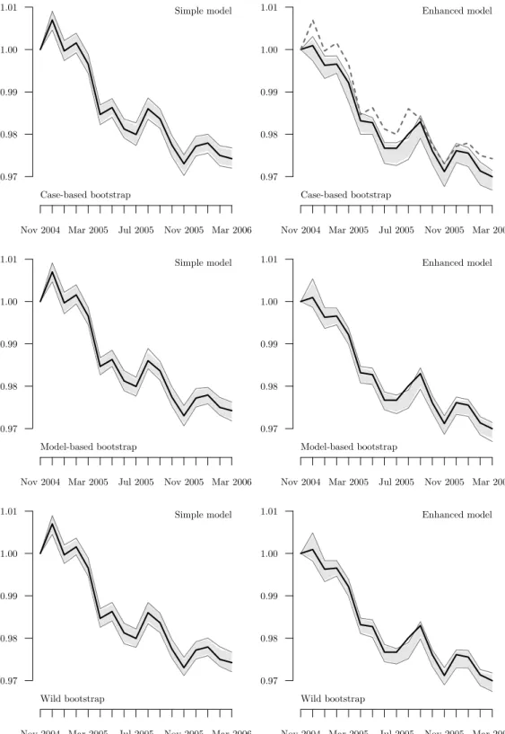
(11) 4.3 Estimating the hedonic indices Bilateral hedonic price indices were estimated using the Jevons formula (7) with the base period 0 being set to November 2004 for all of the estimates. For each month, the pooled characteristics vectors of all the cars available in the base or in the reference period were used as reference characteristics vectors m1 , . . . , mN in order to treat entering and exiting variants symmetrically. The respective sample sizes N are quoted in Table 1. The implementation of the case-based resampling algorithm was straightforward. R = 199 new ˆ0 , h ˆt estimates (h ⋆r ⋆r ) (r = 1, . . . , R) were obtained on the basis of resampled price-characteristics combinations from the original data. The number of replications was chosen such that, when determining the empirical quantiles of ζ⋆0:1 , an integer number of at least five observations was left over at each tail of the distribution. For the OLS estimation of the model coefficients, the model specification was restricted to be the same as the one of the original hedonic function. In other words, all bootstrap replications were built using the same subset of exogenous variables. In the enhanced modelling approach, this principle was applied to each car model individually. Using (12), 90% and 95% confidence intervals for Jevons-type bilateral elementary price indices in all the months under consideration were estimated. These are depicted along with the point estimates of the indices in the top frames of Fig. 1. The variances of the simulated samples have shown to be stable over time leading to almost equal interval lengths (upper minus lower bound) of about 0.4–0.6 percentage points of the index estimate at the 95% level (see Table 1) for both the simple and the enhanced modelling approach. The middle frames of Fig. 1, secondly, present the same type of results for the model-based bootstrap. The main problem here was the proper specification of variance-adjusted residuals. With the choice of a semi-logarithmic model, one implicitly assumes that the variance of the error term ǫt is proportional to (E[P t ])2 while η t , if at all, is homoscedastic. The sampling needs thus to be done on the modified residuals P ˆt t ln ptn − βˆ0t − K t k=1 βk mkn rn = . (15) (1 − hn )1/2 where hn is the nth diagonal element of the hat matrix of model (13). In the enhanced modelling approach, the residuals of the regressions for each car model were modified individually using their specific hat matrix coefficients but then pooled together for generating the bootstrap replications. Consequently, the simulated prices in step 1b of Algorithm 3.2 were set to pt⋆rn = exp(βˆ0t + PK ˆt t t k=1 βk mkn + ǫ⋆n ) accordingly. The results of the wild bootstrap approach, finally, are depicted in the bottom frames of Fig. 1. Here, again, the modified residuals calculated as in (15), and step 1b of Algorithm 3.3 was P were ˆt mt + r t ǫt ) adapted into pt⋆rn = exp(βˆ0t + K β n ⋆rn k=1 k kn As can be seen from Table 1, the interval lengths tend to be somewhat larger on average for the case-based than for the model-based and the wild bootstrap, but the differences are small. Moreover, they are comparable for both modelling approaches of the hedonic function. An interesting observation can be made for the month of August 2005 and the enhanced model. There, the actual index estimate lies outside the 95% bootstrap confidence interval, and this behaviour is similarly reproduced by all three bootstrap algorithms. It seems thus that the point estimate lies at the upper tail of the index distribution.. 11.

(12) 1.01. 1.01. Simple model. 1.00. 1.00. 0.99. 0.99. 0.98. 0.98. 0.97. 0.97 Case-based bootstrap. Nov 2004 Mar 2005. Jul 2005. 1.01. Enhanced model. Case-based bootstrap. Nov 2005 Mar 2006. Nov 2004 Mar 2005. Jul 2005. 1.01. Simple model. 1.00. 1.00. 0.99. 0.99. 0.98. 0.98. 0.97. Nov 2005 Mar 2006 Enhanced model. 0.97 Model-based bootstrap. Nov 2004 Mar 2005. Jul 2005. 1.01. Model-based bootstrap. Nov 2005 Mar 2006. Nov 2004 Mar 2005. Jul 2005. 1.01. Simple model. 1.00. 1.00. 0.99. 0.99. 0.98. 0.98. 0.97. Nov 2005 Mar 2006 Enhanced model. 0.97 Wild bootstrap. Nov 2004 Mar 2005. Wild bootstrap. Jul 2005. Nov 2005 Mar 2006. Nov 2004 Mar 2005. Jul 2005. Nov 2005 Mar 2006. Figure 1: Jevons-type hedonic elementary price index estimates for Nov 2004–Mar 2006 with confidence bands using the case-based, model-based and wild bootstrap approach (from top to bottom) based on R = 199 replications. The solid black line, the shaded area, and the solid grey lines represent the index estimates as well as the 90% and 95% confidence bands respectively. The dashed line in the upper-right frame equals the solid line in the upper-left frame; it is plotted for the sake of easier comparison.. 12.

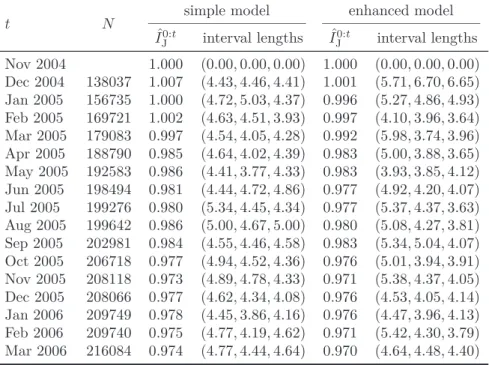
(13) t Nov 2004 Dec 2004 Jan 2005 Feb 2005 Mar 2005 Apr 2005 May 2005 Jun 2005 Jul 2005 Aug 2005 Sep 2005 Oct 2005 Nov 2005 Dec 2005 Jan 2006 Feb 2006 Mar 2006. N. 138037 156735 169721 179083 188790 192583 198494 199276 199642 202981 206718 208118 208066 209749 209740 216084. simple model IˆJ0:t 1.000 1.007 1.000 1.002 0.997 0.985 0.986 0.981 0.980 0.986 0.984 0.977 0.973 0.977 0.978 0.975 0.974. enhanced model. interval lengths. IˆJ0:t. interval lengths. (0.00, 0.00, 0.00) (4.43, 4.46, 4.41) (4.72, 5.03, 4.37) (4.63, 4.51, 3.93) (4.54, 4.05, 4.28) (4.64, 4.02, 4.39) (4.41, 3.77, 4.33) (4.44, 4.72, 4.86) (5.34, 4.45, 4.34) (5.00, 4.67, 5.00) (4.55, 4.46, 4.58) (4.94, 4.52, 4.36) (4.89, 4.78, 4.33) (4.62, 4.34, 4.08) (4.45, 3.86, 4.16) (4.77, 4.19, 4.62) (4.77, 4.44, 4.64). 1.000 1.001 0.996 0.997 0.992 0.983 0.983 0.977 0.977 0.980 0.983 0.976 0.971 0.976 0.976 0.971 0.970. (0.00, 0.00, 0.00) (5.71, 6.70, 6.65) (5.27, 4.86, 4.93) (4.10, 3.96, 3.64) (5.98, 3.74, 3.96) (5.00, 3.88, 3.65) (3.93, 3.85, 4.12) (4.92, 4.20, 4.07) (5.37, 4.37, 3.63) (5.08, 4.27, 3.81) (5.34, 5.04, 4.07) (5.01, 3.94, 3.91) (5.38, 4.37, 4.05) (4.53, 4.05, 4.14) (4.47, 3.96, 4.13) (5.42, 4.30, 3.79) (4.64, 4.48, 4.40). Table 1: Reference characteristics sample sizes, point estimates and lengths of 95% bootstrap confidence intervals for the two modelling approaches. The three interval lengths displayed are those for the casebased, the model-based and the wild bootstrap, respectively, each multiplied by 103 .. 5 Concluding Remarks The results presented in this paper offer some insights into the application of bootstrap methods for evaluating the sampling error of hedonic price indices—an issue which needs to be taken seriously. Three approaches for generating bootstrap replications of hedonic functions have been proposed. Each of them is independent of both the functional form of the hedonic regression and of the choice of a hedonic price index formula. The wild and the model-based bootstrap approaches rely on the availability of varianceadjusted residuals. These may be obtained straightforwardly for linear models. For more sophisticated, non-linear or adaptive, regression models, however, these are in general less easily available. The literature suggests though that linear or semi-linear models might not be sufficient for properly modelling the relationship between characteristics and price of selected goods or elementary aggregates. The empirical analysis in this paper shows that the resulting confidence intervals were virtually identical for all the three bootstrap approaches—in spite of their individual advantages and disadvantages. Thus it appears that the case-based resampling procedure is sufficient and, due to its ease of use, preferable to the two other approaches. An interesting idea for further research might be to estimate confidence intervals for hedonic price indices by inverting a set of hypothesis tests based on bootstrap replications, as this was proposed, e.g., by Davidson and Flachaire (2001, p. 17) or MacKinnon (2002). Furthermore, nonparametric tests for hedonic price indices might be useful for comparing different functional forms of hedonic functions or different specifications of the set of reference characteristics. This paper provides evidence, at least, that these methodical decisions tend to have a larger influence on price index estimates than any variation in the data. The index estimates based on one. 13.

(14) functional form usually did not lie within the confidence intervals of the indices based on the other. What remains clear is the fact that any hedonic price index value is just an estimate of an unknown parameter. Consequently, it contains a certain amount of randomness. Whenever implementing an estimator for hedonic indices, particular attention must be payed to its precision.. References Brachinger, H. W. (2002) Statistical Theory of Hedonic Price Indices. DQE Working Paper 1, Department of Quantitative Economics, University of Freiburg/Fribourg Switzerland. URL http: //ideas.repec.org/p/fri/dqewps/wp0001.html. Court, A. T. (1939) Hedonic Price Indexes with Automotive Examples. In The Dynamics of Automobile Demand, pp. 99–117. General Motors Corporation, New York. Curry, B., Morgan, P., and Silver, M. (2001) Hedonic Regressions: Mis-specification and Neural Networks. Applied Economics 33(5): 659–671. doi:10.1080/00036840122335. URL http://ideas. repec.org/a/taf/applec/v33y2001i5p659-71.html. Davidson, R. and Flachaire, E. (2001) The Wild Bootstrap, Tamed at Last. IER Working Paper 1000, Queen’s Institute for Economic Research, Ontario. URL http://qed.econ.queensu.ca/pub/papers/ abstracts/download/2001/1000.pdf, accessed: 30.09.2005. Davison, A. C. and Hinkley, D. V. (1997) Bootstrap methods and their application. Cambridge Series on Statistical and Probabilistic Mathematics. Cambridge University Press, Cambridge. ISBN 0-52157471-4. Hulten, C. R. (2003) Price Hedonics: A Critical Review. Economic Policy Review 9(3): 5–15. URL http://www.ny.frb.org/research/epr/03v09n3/0309hult.pdf, accessed: 17.05.2004. ILO, IMF, OECD, UNECE, Eurostat, and The World Bank (eds.) (2004) Consumer Price Index Manual: Theory and Practice. International Labour Office, Geneva. ISBN 92-2-113699-X. URL http: //www.ilo.org/public/english/bureau/stat/guides/cpi/. Liu, R. Y. (1988) Bootstrap procedures under some non-I.I.D. models. The Annals of Statistics 16(4): 1696–1708. MacKinnon, J. G. (2002) Bootstrap inference in econometrics. Canadian Journal of Economics 35(4): 615–645. Mammen, E. (1993) Bootstrap and Wild Bootstrap for High Dimensional Linear Models. The Annals of Statistics 21(1): 255–285. Murray, J. and Sarantis, N. (1999) Price-Quality Relations and Hedonic Price Indexes for Cars in the United Kingdom. International Journal of the Economics of Business 6(1): 5–27. doi:10.1080/ 13571519984287. URL http://ideas.repec.org/a/taf/ijecbs/v6y1999i1p5-27.html. Pakes, A. (2003) A Reconsideration of Hedonic Price Indexes with an Application to PC’s. American Economic Review 93(5): 1578–1596. doi:10.1257/000282803322655455. R Development Core Team (2006) R: A Language and Environment for Statistical Computing. R Foundation for Statistical Computing, Vienna. URL http://www.R-project.org. Reis, H. J. and Santos Silva, J. M. C. (2002) Hedonic Prices Indexes for New Passenger Cars in Portugal (1997–2001). Working Paper 10-02, Banco de Portugal Economic Research Department, Lisboa. URL http://ideas.repec.org/p/wpa/wuwpem/0303003.html, accessed: 21.05.2004.. 14.

(15) Triplett, J. E. (2004) Handbook on Hedonic Indexes and Quality Adjustments in Price Indexes: Special Application to Information Technology Products. Working Paper 2004/9, OECD Directorate for Science, Technology and Industry, Paris. doi:10.1787/643587187107. URL http://ideas.repec.org/p/oec/ stiaaa/2004-9-en.html, accessed: 17.09.2005. Venables, W. N. and Ripley, B. D. (2002) Modern Applied Statistics with S . Statistics and Computing. Springer-Verlag, New York, 4th edn. ISBN 0-387-95457-0. Yu, K. (2003) An Elementary Price Index for Internet Service Providers in Canada: A Hedonic Study. Working paper, Department of Economics, Lakehead University, Thunder Bay, Ontario. URL http: //flash.lakeheadu.ca/~kyu/Papers/ISP2001.pdf, accessed: 12.11.2004.. 15.

(16)