Characterizing methane (CH4) emissions in urban environments (Paris)

HAL Id: tel-03230140

https://tel.archives-ouvertes.fr/tel-03230140

HAL is a multi-disciplinary open access

archive for the deposit and dissemination of sci-entific research documents, whether they are pub-lished or not. The documents may come from teaching and research institutions in France or abroad, or from public or private research centers.

L’archive ouverte pluridisciplinaire HAL, est destinée au dépôt et à la diffusion de documents scientifiques de niveau recherche, publiés ou non, émanant des établissements d’enseignement et de recherche français ou étrangers, des laboratoires publics ou privés.

Characterizing methane (CH4) emissions in urban

environments (Paris)

Sara Defratyka

To cite this version:

Sara Defratyka. Characterizing methane (CH4) emissions in urban environments (Paris). Other. Université Paris-Saclay, 2021. English. �NNT : 2021UPASJ002�. �tel-03230140�

Characterization of CH4 emissions in urban

environments (Paris)

Caractérisation des émissions de CH

en milieu

urbain (Paris)

Thèse de doctorat de l'université Paris-Saclay

École doctorale n° 129 Sciences de l’environnement d’Ile-de-France

(SEIF)

Spécialité de doctorat: météorologie, océanographie, physique de l’environnement

Unité de recherche : Université Paris-Saclay, CNRS, CEA, UVSQ, Laboratoire des sciences du climat et de l’environnement Référent : Université de Versailles-Saint-Quentin-en-Yvelines

Thèse présentée et soutenue à Paris-Saclay,

le 19/01/2021, par

Sara DEFRATYKA

Composition du Jury

Valéry CATOIRE

Professeur des universités, Université d’Orléans

Président du jury et Rapporteur

Lilian JOLY

Directeur de Recherche, UMR CNSR Rapporteur et Examinateur

Sébastien BIRAUD

Directeur de Recherche, CESD Examinateur

Valérie GROS

Directrice de Recherche, LSCE Examinatrice

Martina SCHMIDT

Chercheuse, UHEI Examinatrice

Direction de la thèse

Philippe BOUSQUET

Professeur, LSCE Directeur de thèse

Camille YVER-KWOK

Chercheuse, LSCE Invitée, Co- Encadrante de thèse

Jean-Daniel PARIS

Chercheur, LSCE Invité, Co-Encadrant de thèse

Thèse de

doctorat

: 2021

U

PA

SJ0

02

Acknowledgments

First of all, I wish to express my deepest gratitude to Philippe Bousquet, Camille Yver-Kwok and Jean-Daniel Paris for supervising my Ph.D., continuous trust and support, and being wise and brilliant mentors. Philippe, thank you for your enthusiastic and wise guidance and encouraging me to be professional and to look at my work from a bigger perspective. Jean-Daniel, thank you for the intellectual discussions during our surveys which have allowed me to better understand the scientific questions behind my work. Camille, thank you for answering my never-ending questions, helping me improve my skills, and showing me that it is possible to manage both, a scientific career and a family with passion.

Special regards to Valéry Catoire and Lilian Joly for their acceptance to review this thesis. Many thanks to Sébastien Biraud and Valérie Gros for being part of my PhD jury. I am pleased to thank Dave Lowry, Martina Schmidt and Felix Vogel for being my thesis committee members. I value the constructive and developmental discussions we have shared, which progressed my work.

I wish to show my gratitude to the MEMO2 _{European Training Network and Climate Clean Air Coalition Oil}

and Gas Methane Science Studies for financially supporting this thesis and providing the opportunity to participate in informative schools, workshops, and conferences.

I owe much respect to the Royal Holloway University of London Earth Science Department, especially Rebecca Fisher and Euan Nisbet. Also, respects to the UK’s National Physical Laboratory, particularly Rod Robinson and Jon Helmore for serving as my secondment mentors, and for providing a collaborative measurement opportunity with MEMO2_{. Additional thanks to James France for organizing the NPL controlled}

release experiment. Recognition to Jarosław Nęcki and the members of CoMet for allowing me to join an extensive campaign and fulfil my secondment. This experience enriched my knowledge and strengthened skills in the matter of conducting mobile measurements.

I am thank for my LSCE colleagues whose assistance was a milestone in the completion of this project. Thanks to Gregoire and Pramod for assisting me with modelling, explaining different concepts and answering my elementary questions. Thanks to Pierre-Yves and Daniel for numerous hours spent in the car during mobile measurements. Recognition to Abdel and Sebastien who introduced me to secrets of completing a Ph.D. at LSCE and shared useful tips to deal with daily struggles. Also, I am indebted to all of the ICOS team, which always find solutions form any technical problems. Thank you all for time spent during lunch and coffee breaks. Without you, my French articulation would definitely be much lower than today.

From the bottom of my heart, I would like to express immense appreciation for all my substantially supportive friends who were ready to listen my complains whenever I needed it. Barbara and Sophie, thank you for your extensive support during our Social Sundays. Also, a world without unicorns would not be the same. I also want to thank Yunsong for bringing the Ph.D. candidate office large amounts of enthusiasm and energy. Thank you Juli for hosting me during my UK secondments, and numerous hours of interesting discussions. Do not be shy. Malika, thank you for your help with isotopic measurements and data interpretation. Thanks to all MEMO2 _{Ph.D. candidates for creating an amazing and support team of young}

scientists. To my Polish friends, thanks for cheering me up, even from far away, especially Karolcia, Karolina and Piotr who shared their optimism and endless positive energy to get through difficult times. Thanks Ulrich for your endless support and frequent reminders that I am able and ready to finish my Ph.D.

Finally, a very warm thanks to my parents and brother who set me off on the road to my Ph.D. a long time ago. Without their continuous support I would not be able to take on the challenge of doing a Ph.D. Thank you for welcoming me always with open arms and the maximum possible support.

Contents

Figures ... 7

Tables ... 10

Chapter 1 Introduction ... 12

1.1 Global methane budget ... 12

1.2 CH4 sources and sinks ... 13

1.3 Anthropogenic CH4 emissions ... 17

1.3.1 Agriculture CH4 emissions ... 17

1.3.2 Fossil fuels ... 18

1.3.3 Waste management ... 20

1.3.4 Biomass and biofuel burning ... 20

1.3.5 Uncertainties in sectoral CH4 emissions ... 21

1.3.6 Particular role of cities ... 22

1.4 CH4 national and regional emissions – example of France and Île-de-France region ……… 23

1.5 Mitigation action in Île-de-France region ………. 25

1.6 A key role of local mobile measurements ………... 27

1.7 Thesis objectives ………... 28

2 Instrument performance in laboratory and field conditions ………. 30

2.1 Principles of cavity ringdown spectroscopy and analyzer description ………. 31

2.2 Laboratory tests ……….... 32

2.2.1 Initial test ……… 32

2.2.1.1 Continuous measurements repeatability ………..…….. 33

2.2.1.2 Allan deviation ………. 34

2.2.1.3 Short-term and long-term repeatability ……… 34

2.2.1.4 Ambient pressure and temperature dependence ………... 35

2.2.1.5 Calibration ……….. 37

2.2.1.6 C2H6 correction for δ13CH4 ……….……….. 38

2.2.1.7 Initial test - summary ………..………..……….. 40

2.2.2 δ13_CH 4 results from CRDS G2201-i versus IRMS ………..……… 40

2.2.2.1 Continuous simultaneous measurements ……… 41

2.2.2.2 MEMO2 _{isotopic tanks ………... 41}

2.3 Mobile measurements set-up ……….. 44

2.3.1 δ13_CH 4 measured during in-situ mobile measurements ……….….. 46

2.4 Testing of the mobile set-up for δ13_CH 4 ………. 47

2.4.1 Inlet position ………..………. 48

2.4.2 Target gas measurements ……..……….……….. 49

2.4.3 Gas release experiment δ13_CH 4 measure ……….……… 49

3 Ethane measurement by Picarro CRDS G2201-i in laboratory and field conditions: potential and limitations ………..………. 53

3.1 Introduction ……….. 53

3.2 Publication: Ethane measurement by Picarro CRDS G2201-i in laboratory and field conditions: potential and limitations ………..……….. 55

4 Mapping urban methane sources in Paris, France ………..………. 80

4.1 Introduction: motivation and summary of the publication ………..……….. 80

4.2 Observation of temporal variation within mapping urban methane sources in Paris ....………… 82

5 Direct estimation of methane emissions from gas compressor stations and landfills in Île-de-France 104

5.1 Introduction ………..……… 104

5.2 Methods used on site scale ……….……… 106

5.2.1 Isotopic signature ………..……… 106

5.2.2 Ethane to methane ratio ……….. 106

5.2.3 Emission rate ………. 107

5.2.3.1 Gaussian model in the Polyphemus platform ………. 107

5.2.3.2 Gaussian model in Polyphemus platform- controlled release experiment 110 5.2.3.3 Tracer dispersion method ………. 113

5.2.3.4 Tracer dispersion method – example of application ……….…… 116

5.3 Application of direct measurements methods in Île-de-France ……….……….. 121

5.3.1 Gas compressors stations ……… 122

5.3.1.1 Gas compressor station A ………. 122

5.3.1.2 Gas compressor station B ………. 124

5.3.1.3 Gas compressor station C ………. 126

5.3.2 Landfills ………..……….. 130

5.3.2.1 Landfill D ……….……….. 131

5.3.2.2 Landfill E ………..………..………..… 133

5.3.3 Other proxies for partitioning CH4 sources – ethane to methane ratio and δDCH4 ……….………..………..……… 134

5.4 Synthesis and discussion ……….………. 136

6 Conclusions and Outlooks ………..……… 139

6.1 Conclusions ….………..………. 139

6.2 Outlooks ………..………. 143

List of abbreviations ………..………..……….. 147

References ……….………..………. 148

Appendix A: Supplementary information to Mapping urban methane sources in Paris, France .………. 159

Figures

Figure 1.1 From Saunois et al. 2020: Globally averaged atmospheric CH4 (a) and its annual growth rate GATM

(ppb yr-1_{) (b) from four measurements programs, National Oceanic and Atmospheric Administration}

(NOAA), Advanced Global Atmospheric Gases Experiment (AGAGE), Commonwealth Scientific and

Industrial Research Organization (CSIRO), and University of California, Irvine (U.C.I.). ……….. 12

Figure 1.2 From Sherwood et al. 2017: Genetic characterization plot of δDCH4 (δ2H) versus δ13CH4 (δ13C). M: microbial; T: thermogenic; A: abiotic; MCR: microbial CO2 reduction; MAF: microbial acetate fermenta-tion; ME: microbial in evaporitic environment; TO: thermogenic with oil; TC: thermogenic with condensate; TD: dry thermogenic; TH: thermogenic with high-temperature CO2–CH4 equilibration; TLM: thermogenic low maturity; GV: geothermal–volcanic systems; S: serpentinized ultramafic rocks; PC: Precambrian crystalline shields. ……….……….. 15

Figure 1.3 From Saunois et al. 2020: Global Methane Budget for the 2008-2017 decade. Both bottom-up (left) and top-down (right) estimates are provided for each emissions and sink category in Mt CH4 yr-1 (Tg CH4 yr-1_{), as well as for total emissions and total sinks. ……….………. 17}

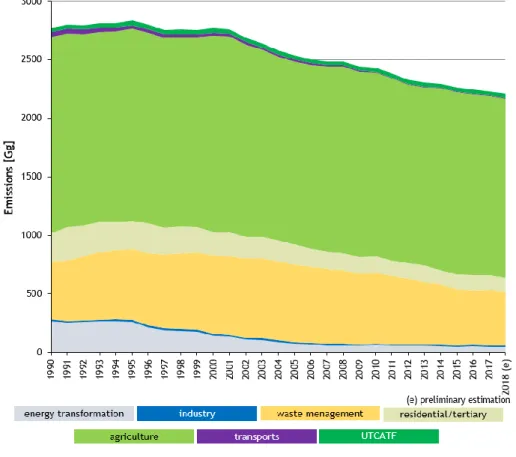
Figure 1.4 From CITEPA, 2019: Evolution of the CH4 emissions in Metropolitan France since 1990 .……… 23

Figure 1.5 Sectoral contribution to IDF region emissions in the year 2015, (AIRPARIF 2018) ……….. 24

Figure 2.1 Scheme of light intensity decay over time in CRDS analyzer. ……….. 31

Figure 2.2 CMR test provided for instrument CFIDS 2072. Left: CH4 mixing ratio [ppb], right: δ13CH4 isotopic signature [‰] ………...……… 33

Figure 2.3 Allan deviation for instrument CFIDS 2072. Left: CH4 mixing ratio [ppb], right: δ13CH4 isotopic signature [‰] ………...……… 34

Figure 2.4 Repeatability for instrument CFIDS 2072. Left: short-term repeatability, right: long-term repeatability. Top: CH4 mixing ratio [ppb], bottom: δ13CH4 [‰] ……….… 35

Figure 2.5 Ambient pressure and temperature dependence for instrument CFIDS 2072. Left: pressure dependence, Right: temperature dependence. Top: CH4 mixing ratio [ppb], bottom: δ13CH4 [‰]. ……….. 36

Figure 2.6 The calibration history for CFIDS 2072 over two years. Left: CH4 mixing ratio [ppb], right: δ13CH4 [‰] .……….. 37

Figure 2.7 From Rella et al. 2015: Spectra of key species in the frequency ranges employed in the spectrometer, displaying loss on a log scale vs. optical frequency in wavenumbers for the low-frequency region (around 6029cm-1_{) ……….……… 38}

Figure 2.8 From Assan et al. 2017: Set-up used to determine C2H6 correction for δ13CH4 ……… 39

Figure 2.9 The effect of C2H6 on reported δ13CH4. ………. 39

Figure 2.10 CRDS 2072 and RHUL IRMS comparison. 20 minutes’ averages CRDS value with calibration, without C2H6 correction, error bars represent 1 standard deviation of CRDS measurements ……….. 41

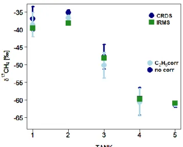
Figure 2.11 Comparison δ13_CH 4 value IRMS and CRDS, with CRDS 2072 calibration and C2H6 correction, error bars represent 1 standard deviation ………..… 43

Figure 2.12 Scheme of mobile measurement set-up. The blue arrows show the airflow in monitoring mode. The green arrows show the airflow in the replay mode. ………....………...… 44

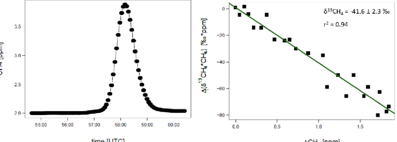
Figure 2.13 The scheme of methods used during mobile measurements ……… 45 Figure 2.14 Example of AirCore sample. Left: CH4 plume measured in replay mode, right: Miller-Tans plot 47

Figure 2.15 Observed mixing ratio at the lower and upper inlets; left panel: CH4 mixing ratio over time, dotted

lines indicate a time when car was parked. Right panel: correlation lower - upper inlet during comparison inlet position with subtracted time when the car was parked. The red line corresponds to y=x. The green line shows the linear fitting ………..… 48

Figure 2.16 Tank measurement before/after mobile measurements between December 2018 and June 2019.

The dotted line marks mean value over measurement period. Error bars represent 1 standard deviation, left: CH4 over the time; right: δ13CH4 over the time. ……… 49

Figure 2.17 Determined δ13_CH

4 from bag samples. Left Keeling plot, right: Miller-Tans plot. Error bars

represent 1 standard deviation. ………..……….… 50

Figure 2.18 Determined δ13_CH

4 from in situ mobile measurements. Left without C2H6 correction, right: with

C2H6 correction ……….………… 51

Figure 4.1 Comparison of observed CH4 mole fraction between September 2018 and March 2019 (plots a)

and c)) and summer 2019 (plots b) d)). Top: observed CH4 mixing ratio above background. Bottom:

determined leak indications ……….…… 83

Figure 5.1 Example of transects made downwind from the source during the controlled release experiment.

CH4 enhancement above background is presented. Left: map with made downwind transects; red point –

release tower, white point – meteorological station, black point – the beginning of the model window set in Polyphemus. Transects are made in three different distances (A, B, C). Right: Observed CH4

enhancement in three different distances from source ……….……… 111

Figure 5.2 Example of individual transect, release 15 transect 8. Red point – release tower, black point – the

beginning of model window set in Polyphemus. CH4 enhancement above background is shown. Left:

measurement while crossing a peak. Right: Gaussian model; top: modeled dispersion, bottom: comparison of modeled and measured CH4 mixing ratio. ……….… 111

Figure 5.3 Release 15. Example of measured (top) vs. modeled (bottom) plumes for three different distances.

CH4 enhancement above background is presented. X axis represents distance from the beginning of the

model window set in Polyphemus. Note that scale used for distance A differs from scales for distance B and C. ……… 112

Figure 5.4 Emission rate calculated for individual transects. Left: source height 4.37m, right source height 0.1

m. In both plots, two first measurements were made with a dryer before the instrument inlet, while the next two – without a dryer. ……… 112

Figure 5.5 Based on Lamb (1995): Scheme of the tracer dispersion method during mobile measurements with

analyzer situated inside the car. ……….… 114

Figure 5.6 Koedijk gas compressor station. a) localization b) CH4 mixing ratio observed during survey on

12.02.2018 c) CH4 mixing ratio during one individual transect d) C2H2 mixing ratio during one individual

transect. Figure c) and d): red circles – probable CH4 sources, black dot – C2H2 cylinder position. The

background is not subtracted. ………. 116

Figure 5.7 CH4 and C2H2 mixing ratio measured on the Koedijk gas compressor station, 12.02.2018. Left:

Figure 5.8 Modeled dispersion for first meteorological condition (1st _{transect) using GRAL model, Koedijk gas}

compressor, 12.02.2018. The presented grid map is larger than the simulation area, and there are no simulated particles in the bottom part of the map. Left: simulated dispersion for C2H2. Right: simulated

dispersion for CH4 ………. 118

Figure 5.9 Koedijk gas compressor, 12.02.2018 Comparison of model and measurement of 9th _{peak. Left:}

C2H2. Right: CH4 ………....… 118

Figure 5.10 Gaussian model results for transect 9th_{, Koedijk gas compressor, 12.02.2018, Top: Modeled}

dispersion for 9th _{meteo condition. Bottom: Comparison of Model and observation. a) and c) C}

2H2 results

b and d) CH4 results ………. 119

Figure 5.11 The location of landfills and gas compressors surveyed during the Ph.D. study ……… 121 Figure 5.12 Gas compressor A. Observed CH4 mixing ratio. The white number indicate δ13CH4 [‰].

Background is not subtracted. c) and d) present CH4 mixing ratio on 15.07.2010 when the emission rate

was estimated. d) multiple crossing of the CH4 plume. ……… 123

Figure 5.13 Gaussian model results for transect 16th_{, gas compressor A, 15.07.2019, Top: Spatial dispersion}

of CH4 concentration, bottom: Comparison of model and observation. a) and c) stability class A b and d)

stability class B ……… 124

Figure 5.14 Gas compressor station B observed CH4 mixing ratio. The white number indicates δ13CH4 [‰].

Background is not subtracted. ……….………… 125

Figure 5.15 Gas compressor station C. Observed CH4 mixing ratio above background. The white numbers

indicate δ13_CH

4. Background is not subtracted. b) multiple crossing of the CH4 plume. ……… 127

Figure 5.16 Gas compressors C, 29.05.2019. a) Observed CH4 mixing ratio with rose wind b) multiple crossing

of the CH4 plume. Background is not subtracted ……….………… 128

Figure 5.17 Gaussian model results for transect 29th_{, gas compressor station C, 29.05.2019, Top: Spatial}

dispersion of CH4 concentration, bottom: Comparison of model and observation. a) and c) stability class

A b and d) stability class B. ………..………… 129

Figure 5.18 Landfill D, 10.01.2019. a) Observed CH4 mixing ratio above background. The white numbers

indicate δ13_CH

4 measured inside landfill (27.11.2018) and outside landfill (10.01.2019). b) multiple

crossing of the CH4 plume. Background is not subtracted ………. 131

Figure 5.19 Landfill D, 06.10.2017, observed mixing ratio. Example of individual transect. Left: CH4 mixing

ratio. Right: C2H2 mixing ratio. Background is not subtracted. ……… 132

Figure 5.20 Landfill E, observed CH4 mixing ratio above background. The white numbers indicate δ13CH4 [‰].

Tables

Table 2.1 CMR test results for CFIDS 2072 and CFIDS 2067 ……… 33 Table 2.2 Allan deviation results for CFIDS 2072 and CFIDS 2067 ………. 34 Table 2.3 Repeatability for CFIDS 2072 and CFIDS 2067 ………..……… 35 Table 2.4 Ambient pressure and temperature dependence CH4 mixing ratio and δ13CH4 isotopic signature

for CFIDS 2072 and CFIDS 2067 ………..……….….. 36

Table 2.5 Linear regression coefficients of calibration test calculated for CFIDS 2072 ………..………… 37 Table 2.6 Linear regression coefficients calculated for C2H6 correction for δ13CH4 ……… 39

Table 2.7 Comparison δ13_CH

4 value IRMS and CRDS, with CRDS 2072 calibration ………. 43

Table 2.8 CH4 and δ13CH4 from tank measurement before/after mobile measurements between December

2018 and June 2019

.

Table 2.9 Isotopic signature determined during in situ mobile measurements ……….. 52 Table 4.1 Comparison of CH4 observed in Paris between September 2018 and March 2019

with Summer 2019 ………. 84

Table 5.1 Meteorological conditions defining Pasquill – Turner stability classes (Pasquill 1961). ……… 108 Table 5.2 Diffusion equations for Briggs formula for the rural area as a function of Pasquill – Turner stability

class and downwind distance from the source (Briggs 1973) ………. 108

Table 5.3 Diffusion equations for Briggs formula for the urban area as a function of Pasquill – Turner stability

class and x downwind distance from the source (Briggs 1973) ……….. 108

Table 5.4 CH4 emission rate calculated using the Gaussian model on the Polyphemus platform. Emission rates

are calculated in L CH4 min-1n ……….… 112

Table 5.5 Estimated emission for each transect during measurement on Koedijk gas station ……… 117 Table 5.6 CH4 and C2H2 emission rate calculated for Koedijk gas compressor, 12.02.2018 ……… 120

Table 5.7 δ13_CH

4 observed for gas compressor station A. CRDS results in this study are determined using the

AirCore tool. For IRMS measurements, bag samples were taken and sent to UU. ……… 123

Table 5.8 δ13_CH

4 observed for gas compressor B. CRDS results in this study are determined using the AirCore

tool. For IRMS measurements, bag samples were taken and sent * to RHUL or ** to UU. ……… 125

Table 5.9 δ13_CH

4 observed for gas compressor C. CRDS results in this study are determined using the AirCore

tool. For IRMS measurements, bag samples were taken and sent * to RHUL or ** to UU. ……… 128

Table 5.10 δ13_CH

4 observed for landfill D. CRDS results in this study are determined using the AirCore tool,

*** measured during crossing plume. For IRMS measurements, bag samples were taken and sent * to RHUL or ** to UU. ………. 132

Table 5.11 CH4 emission calculated on landfill D over time using the tracer release method. ……… 132

Table 5.12 δ13_CH

4 observed for landfill D. CRDS results in this study are determined using the AirCore tool.

Table 5.13. From Defratyka et al. (2020): Ratio measured at different gas compressor stations (A, B) and a

landfill (D); Numbers after identification letters refer to different surveys. ΔCH4 and ΔC2H6 are defined as

the difference between background value (1st _{percentile) and the observed value inside the peak …… 135}

Table 5.14 δDCH4 observed in IDF. Bag samples were taken and sent to UU. ……… 136

Table 5.15 Characteristics of three gas compressors (A, B, C) and two landfills (D, E) in the IDF region. δ13_CH 4,

Chapter 1 Introduction

1.1

Global methane budget

Methane (CH4) is one of the greenhouse gases that occur naturally in the atmosphere. However,

its global mean mixing ratio has increased about 2.6 times compared to the pre-industrial times (IPCC 2018; Saunois et al. 2019; Turner et al. 2019) and reached 1880 ppb in July 2020 (Dlugokencky 2020). According to the ice core measurements, over the last millennium before the pre-industrial times, the methane mixing ratio varied around 700 ppb (IPCC 2018; Turner et al. 2019). Moreover, after a short period of stabilization around 1775 ppb, between 2000 and 2007, the atmospheric methane rose again by up to 7.7 ± 0.7 ppb/ year in 2017 (Nisbet et al. 2019). Current CH4 trend places CH4 emissions close

to the warmest IPCC-AR5 scenario (RCP8.5 scenario) (Saunois et al. 2016; Jackson et al. 2020). Following this trajectory causes a temperature increase above 3 °C by the end of the century (Saunois et al. 2020). It will thus require an extensive reduction of the methane emissions to limit the temperature rise to 1.5-2 °C from the Paris Agreement (Nisbet et al. 2019). The observed global trend of CH4 concentration is presented in Fig 1.1.

Figure 1.1 From Saunois et al. 2020: Globally averaged atmospheric CH4 (a) and its annual growth rate

GATM (ppb yr-1_{) (b) from four measurements programs, National Oceanic and Atmospheric}

Administration (NOAA), Advanced Global Atmospheric Gases Experiment (AGAGE), Commonwealth Scientific and Industrial Research Organization (CSIRO), and University of California, Irvine (U.C.I.).

At current atmospheric concentration, methane global warming potential (GWP) is higher than for carbon dioxide (CO2) and for a 100-year timeline without considering climate feedback, its GWP is

28 times higher than for CO2 (IPCC 2018). Additionally, CH4 has a shorter lifetime than CO2 and in 2010

was about 9 years (Voulgarakis et al. 2013; Morgenstern et al. 2017). Therefore, CH4 mitigation actions

result in relatively fast stabilization or reduction of atmospheric CH4 mixing ratio, which can be an

efficient way to reduce the global greenhouse gas effect on the decennial time scale (Saunois et al. 2019; Nisbet et al. 2019; Turner et al. 2019).

Implementing efficient mitigation actions requires a good knowledge about the CH4 emissions,

both on the local and global scale. Determination of CH4 budget can be done using bottom-up or

atmospheric chemistry from process-based models, inventories of anthropogenic emissions and data extrapolation. In the case of the inventories, emissions are estimated as multiplication of activity data by emission factors, while activity data are determined based on statistical surveys and default emissions factors are stated by the IPCC guidelines (IPCC 2006). In the case of the bottom-up estimations, obtained values can vary widely depending on the used inventories. This is due to the discrepancy between used activity data and different categorizations in individual inventories. Also, used emission factors may not indicate specific conditions in individual countries in different emission sectors (Saunois et al. 2016).

The top-down studies are based on atmospheric observation within the inverse-modeling network. In the case of top-down studies, the contribution of each particular source to total CH4

emissions can be difficult to determine (Saunois et al. 2019; Turner et al. 2019).

1.2

CH

4

sources and sinks

According to Saunois et al. (2020), using top-down approach, estimated CH4 total global emissions

was equal to 572 Mt CH4 yr-1 [538-593] (mean, [min - max]) for 2008- 2017, where for bottom-up

studies it was ~25% higher and reached 737 Mt CH4 yr-1 [593- 880] for the same period. Using a

top-down approach, on a global scale, the uncertainty is about 5%. However, looking at the latitudinal distribution, uncertainty doubles for the tropic and the northern mid-latitudes and it increases to more than 25% in the northern high-latitudes. Based on top-down studies, tropical emissions constitute the biggest contribution to the global CH4 emissions (~64%), where mid-northern and high-northern

latitudes contribute, respectively, ~32% and ~4% (Saunois et al. 2020).

Going from the global scale to individual emitters, methane sources can be divided into categories by emissions processes (biogenic, thermogenic or pyrogenic) or by partitioning methane between natural/anthropogenic sources. Regarding emissions processes, decomposition of organic matter by methanogenic Archaea produces biogenic methane by CO2 reduction or by acetate fermentation

(Whiticar 1999). Biogenic processes occur in anaerobic environments, such as rice paddies, landfills, sewage and wastewater treatment facilities, water- saturated soils, marine sediments, swamps or ruminants’ digestive system.

Thermogenic methane is created on the geological timescales. It is formed by the breakdown of buried organic matter through pressure and heat deep in the Earth’s crust. It is released to atmosphere through land and marine geological gas seeps, including exploitation of fossil fuels. Pyrogenic methane reaches the atmosphere due to the incomplete combustion of biomass and other organic material. Incomplete combustion occurs in wildfires, peat fires, biomass burning in degraded or deforested areas and biofuel burning (e.g., Whiticar 1999; Sherwood et al. 2017; Milkov and Etiope 2018; Saunois et al. 2020).

Studying isotopic signature of methane released to atmosphere extends the knowledge about methane formations. Methane isotopic signature is commonly reported in δ notation, which quantifies relative deviation of isotope ratio and it is expressed in parts per mil (‰). The isotopic signature is calculated as:

𝛿 = (𝑅𝐴

where RA is the isotopic ratio of the measured methane sample and Rstd is the isotopic ratio of the

standard gas. Typically, the isotopic ratio represents the ratio of the rare isotope to abundant isotope, like 13_C/12_{C or} 2_H/1_{H. To report δ(}13_{C, CH}

4) values, Vienna Pee Dee Belemnite international standard is

used (VPDB, 13_R

VPDB = 0.0112372) (Craig 1957), while Vienna Standard Mean Ocean Water (VSMOW, 2_R

VSMOW = 0.0020052) (Baertschi 1976) is an international standard for δ(D, CH4). In the manuscript,

δ(13_{C, CH}

4) and δ(D, CH4) are abbreviated as δ13CH4 and δDCH4.

Isotopic signature varies globally and depends from different factors (e.g., location, formation or management in the case of anthropogenic sources.). Lower δ13_CH

4 value (range -80 ‰ to -40 ‰) are

connected with biogenic sources like waste disposal and landfill, wastewater treatment or agriculture, as methanogenic bacteria are highly selective for 12_{C. Biogenic methane from CO}

2 reduction is more 13_{C depleted than from acetate fermentation (Whiticar 1999). Depending from the origin of natural}

gas, which is dominantly a thermogenic source, its isotopic composition varies between -75 ‰ and -25 ‰. Thermogenic methane become more 13_{C enriched at high maturity stages (Sherwood et al.}

2017). Enriched δ13_CH

4 (between -35 ‰ and -7 ‰) come from pyrogenic sources like combustion in

energy production or heating. The variety in isotopic signature of pyrogenic sources is related to the type of burned organic material (Chanton et al. 2000).

As δ13_CH

4 can overlap between processes, δDCH4 can be used as additional proxy to determine

methane origin. Based on the study of Sherwood et al. (2017), where different isotopic signatures over the world are collected, δDCH4 for biogenic sources is about -317 ‰ (range -442 ‰ to -281 ‰).

Pyrogenic and thermogenic methane is more δDCH4 enriched. For thermogenic methane, mean δDCH4

is equal to -197 ‰ (range – 415 ‰to -62 ‰), while for pyrogenic sources it reaches - 211 ‰ (range -232 ‰ to -195 ‰). Again, some δDCH4 values overlap for different processes. Genetic

characterization plot of δ13_CH

4 and δDCH4 can be used to better distinguish methane of different origin

(Sherwood et al. 2017; Milkov and Etiope 2018; Whiticar 1999). Figure 1.2 presents an example of application of genetic characterization plot used in study made by Sherwood et al (2017). Methane produced in these three processes has both anthropogenic and natural origin (Nisbet et al. 2019; Turner et al. 2019; Saunois et al. 2020; Jackson et al. 2020).

Methane can also contain 14_{C, which is a radioactive isotope with 5730 years of half-life.}

Radiocarbon (14_{C) is constantly produced in the upper atmosphere by cosmic rays and its}

concentration remains stable. In the atmosphere, cosmic rays collide with nuclei and liberate neutrons. In the next step, theses neutrons replace one of the 7 protons in the nitrogen nuclei. As a result, the new atom of 14_{C is created, which contains 6 protons and 8 neutrons. All living organisms}

contain radiocarbon due to carbon exchange via, for example, photosynthesis process and food chain. After death, their radiocarbon concentration decreases due to radioactive decay. Thus, 14_{C allows to}

distinguish fossil fuel emissions as they are almost completely depleted in 14_{C, cause they were}

separated from atmosphere over a very long time (e.g., Lowe et al. 1991). Currently measurements of

14_{C remains scarce as they require a bigger measurement volume and advanced laboratory equipment}

(e.g., Townsend-Small et al. 2012; Espic et al. 2019; Turner et all. 2019).

Additionally, clumped isotopes (rarer isotopes substitute part of the molecules, such as 12_CH 2D2 or 13_CH

3D) can be used to separate biogenic/thermogenic emissions or the CH4 loss trough reaction with

OH (Stolper et al. 2014; Haghnegahdar et al. 2017). However, the determination of different clumped isotopes requires expensive and technically advanced measurements technique, and currently, it is not applied for continuous measurements (Turner et al. 2019).

Not only measurements of isotopes can give additional source information. For instance, carbon monoxide (CO) is co-emitted during incomplete combustion. Due to that, it can be a proxy of the methane emissions from biomass burning (Saunois et al. 2020). Ethane (C2H6) is a co-component of

the fossils fuels, and it is co-emitted during the extraction of coal, oil and natural gas (Simpson et al. 2012; Turner et al. 2019). Additionally, the ethane to methane ratio varies depending on the facility and type of fossil fuel (Lopez et al. 2017; Yacovitch et al. 2014). Also volatile organic compounds (VOC) are co-emitted with natural gas and oil extraction and production. Lighter VOCs are released with natural gas, while heavier VOCs are co-emitted with oil (Warneke et al. 2014). For example, isomeric pentane ratio (i-pentane/n-pentane) can be used to characterise oil and natural gas activities, vehicle emissions and other urban emissions (Baker et al. 2008; Thompson et al. 2014). As propane is also co-emitted during natural gas and oil activities, it can also be used as additional indicator (e.g., Helmig et al. 2016).

Figure 1.2 From Sherwood et al. 2017: Genetic characterization plot of δDCH4 (δ2H) versus δ13CH4

(δ13_{C). M: microbial; T: thermogenic; A: abiotic; MCR: microbial CO}

2 reduction; MAF: microbial acetate

fermentation; ME: microbial in evaporitic environment; TO: thermogenic with oil; TC: thermogenic with

condensate; TD: dry thermogenic; TH: thermogenic with high-temperature CO2–CH4 equilibration; TLM:

thermogenic low maturity; GV: geothermal–volcanic systems; S: serpentinized ultramafic rocks; PC: Precambrian crystalline shields.

Based on top-down studies, the anthropogenic activities contribute 359 Mt CH4 yr-1 or 60% (range

from 55 to 70%) of the total global emissions and natural emissions contribute 40%. Based on the bottom-up approach, the estimated emissions from natural sources are higher than using the top-down approach. Estimated emissions from natural and anthropogenic sources are more balanced, and their contribution is about 50% each. The equal contribution from natural and anthropogenic sources is not consistent with ice cores studies. Ice core and atmospheric methane data confirm the current predominant role of anthropogenic methane (Nicewonger et al. 2016; Turner et al. 2019; Saunois et al. 2020). For natural emissions, the wetlands play a crucial role (178 Mt CH4 yr-1, top-down study),

where biofuel and biomass burning and other natural emissions (e.g., other inland waters, termites, wild animals) have a smaller contribution to natural CH4 emissions. Notably, the biggest discrepancy

between top-down and bottom-up approaches comes from the "other natural emissions" (37 Mt CH4

yr-1 _{vs. 222 Mt CH}

4 yr-1). Discrepancy between this two approaches can be caused by the lack of some

sources of “other natural emissions” like freshwater or permafrost in top-down studies. Moreover, in the case of bottom-up studies, the two biggest contributors, freshwaters (~75%) and geological emissions (~15%) have large uncertainties (Marielle Saunois et al. 2020).

The emissions categories as biomass and biofuel burning have both natural and anthropogenic origin (30 Mt CH4 yr-1). However, 42% of anthropogenic emissions come from agriculture and waste

sector (219 Mt CH4 yr-1,top-down study) and fossil fuel production and use (109 Mt CH4 yr-1, top-down

study) contribute 31% of anthropogenic emissions. Looking for the uncertainty of the estimated emissions, using the top-down approach, the uncertainty is larger for estimated anthropogenic emissions. In contrast, for wetland emissions, uncertainty is larger using the bottom-up approach (Marielle Saunois et al. 2020).

The global CH4 budget, including sources and sinks divided by sectors, is presented in figure 1.3.

CH4 emissions come from natural or anthropogenic sources that are partly balanced by four sinks.

Total mean global loss of methane is equal to 625 Mt CH4 yr-1 (bottom-up study) or 556 Mt CH4 yr-1

(top-down study). To determine CH4 sinks, most of the top-down models use the same OH distribution

from TRANSCOM experiment. The TRANSCOM experiment was dedicated to intercomparison of chemistry-transport models to investigate the roles of surface emissions, transport and chemical loss in simulating the global methane distribution (Patra et al. 2011). In the case of bottom-up studies, methane sinks and lifetime can be estimated using global model results from the Chemistry Climate Model Initiative (CCMI) (Morgenstern et al. 2017). Oxidation by the hydroxyl radical (OH), mostly in the troposphere, amounts to 90% of the total sinks (Saunois et al. 2020; Turner et al. 2019). Photochemistry loss in the stratosphere is another atmospheric sink of the CH4. In the stratosphere,

methane removal occurs by reactions with OH, O1_{D (excited oxygen atoms), atomic Cl and atomic F.}

The oxidation in soils and chlorine photochemistry in the marine boundary layer are the two remaining CH4 sinks. Atmospheric chemistry models are used to determine uncertainty of total methane sink.

The uncertainties are about 20%-40% and decrease to 10%-20% when atmospheric proxy methods are used (e.g., methyl chloroform) (Saunois et al. 2016).

Figure 1.3 From Saunois et al. 2020: Global Methane Budget for the 2008-2017 decade. Both

bottom-up (left) and top-down (right) estimates are provided for each emissions and sink category in Mt CH4

yr-1 _{(Tg CH}

4 yr-1), as well as for total emissions and total sinks.

Overall, using top-down approach, estimated CH4 total global emissions reached 572 Mt CH4 yr-1

[538-593] for 2008- 2017. For bottom-up studies it was ~25% higher and reached 737 Mt CH4 yr-1 [593-

880] for the same period. This discrepancy can be caused by using OH distribution from TRANSCOM experiment, which leads to constrained global budget. Likely, the bottom-up budget is overestimated due to up-scaling of local measurements and double-counting of some sources (e.g. wetlands with other natural sources.).

In the following, anthropogenic sources are presented in details, as this Ph.D. study is focused on anthropogenic CH4 characterization at local scale. Studies on anthropogenic CH4 emissions allow for

taking effective mitigation action to reduce atmospheric CH4. Reductions of natural CH4 emissions are

more complex cases as they can affect in negative environmental feedback (e.g. drying of wetlands could disturb ecosystems) and it is not described here. It is worth to note that in the northern mid-latitudes, anthropogenic emissions play a dominant role. At the same time, the agriculture and waste sector contributes to 42% of total anthropogenic emissions, followed by the contribution of fossil fuel emissions (31% of total anthropogenic emissions).

1.3

Anthropogenic CH

4

emissions

1.3.1

Agriculture CH

emissions

Agricultural emissions reached 141 Mt CH4 yr-1 [131 Mt CH4 yr-1 -154 Mt CH4 yr-1] over 2008-2017

(bottom-up study) and are mostly connected with livestock production and rice cultivation. For livestock production, the emissions come from enteric fermentation and manure management.

Saunois et al. (2020), using the bottom-up approach, estimated emissions for livestock production (including enteric fermentation and manure management) to 111 Mt CH4 yr-1, with range 106-116 Mt

CH4 yr-1 for a period 2008-2017.

In the case of enteric fermentation, methane is a product of the anaerobic microbial activity in the digestive system of domestic ruminants (e.g., cattle, buffalo). Globally, cattle contribute to the majority of enteric fermentation, due to the large population (~1.4 billion). The methane emissions from the enteric fermentation can vary depending on the country because of different living conditions and the agriculture system (Reay et al. 2010; USEPA 2012; Saunois et al. 2020).

Methane emissions from the manure depends on the manure management system, which affects anaerobic conditions of manure decomposition. For example, handling manure as a solid or depositing it on pasture fosters aerobically decomposition, which results in small or null CH4 production.

Moisture, ambient temperature, residency time, or manure composition also affect the growth of methanogenic bacteria. For example, moisture can foster CH4 formation when dry storage is provided.

The type of diet affects manure composition and typically, higher-energy feed can cause larger methane production (USEPA 2012).

Rice cultivation is the next source of methane in agriculture. As most of the rice grows in flooded paddy, changing the water management system is one of the potent ways to mitigate CH4 emissions

(e.g., seasonally drainage). For the period 2008-2017, rice cultivation contributes to 8% of total anthropogenic emissions of methane (30 [25-38] Mt CH4 yr-1) (USEPA 2012; Saunois et al. 2020).

1.3.2

Fossil fuels

The second most significant sector of the anthropogenic methane emissions is connected with fossil fuel (natural gas, oil, and coal) production and use. It contributes to 35% of global anthropogenic emissions and reached 128 [113 - 154] Mt CH4 yr-1 over 2008-2017. The coal mining emissions

contribute, on average, to 33% of total fossil fuel emissions of methane (42 [29-60] Mt CH4 yr-1)

(Marielle Saunois et al. 2020). Methane is trapped within coal seam and surrounding rock strata over coalification process and can be emitted by natural erosion or by mining operation (USEPA 2012). In underground coal mines, methane emissions come from the shafts' ventilation where air is pumped into the mine to hold the methane mixing ratio < 0.5%. Methane emitted during ventilation can be used as a fuel, however in some countries it is still released to the atmosphere or flared. In the case of surface mining, methane is directly released to the atmosphere (USEPA 2012). Moreover, CH4 is

also emitted during processing and post-processing mining activities and transportation. The abandoned mines and coal waste piles are also sources of methane. They are higher than it was assumed in the past and they count for about 20% of emissions from functioning mines (Saunois et al. 2020).

In the case of oil and natural gas exploitation, methane emissions occur from conventional gas and oil as well as from shale gas exploitation and contribute ~63% of total fossil fuel emissions (76 [66-92] Mt CH4 yr-1) (Saunois et al. 2020). Methane is a main component of natural gas (~95%) and it

is released to the atmosphere through natural gas extraction, processing, distribution and transmission. Natural gas often occurs with petroleum deposits. Thus, methane is also emitted during extraction and upstream production of oil (USEPA 2012). After the Madrid forum (“Potential ways the

gas industry can contribute to the reduction of methane emissions”, 5-6 June 2019), the GIE report (Gas Infrastructure Europe) synthesized information and data on European CH4 emissions of the entire

natural gas value chain. The GIE report provides three types of the methane emissions from natural gas industry: fugitives, venting and incomplete combustion (GIE and MARCOGAZ 2019). Fugitive emissions come from the unintended leaks in the infrastructure and can be challenging to determine, depending on their magnitude. During venting, planned releases of methane occur. Methane is emitted for safety reasons, operational procedures or equipment design. Incomplete combustion can occur in the exhaust of natural gas combustion equipment (GIE and MARCOGAZ 2019). Nowadays, in some oil and gas facilities, venting of the natural gas is replaced by flaring with conversion to CO2.

During the oil extraction, natural gas is emitted as well. It can be recovered for utilization as an energy source or re-injection or not recovered. Thus, it is flared or vented. The recovery rate of natural gas from oil extraction varies from country to country. It is the highest in the U.S., Canada, and Europe (Saunois et al. 2020).

Besides the conventional extraction of oil and natural gas, the exploration of shale gas has become more popular over last decades. The extraction of natural shale gas started in the 1980s in the U.S. and since the beginning of this century, the production developed on a large scale and in 2017 reached 62% of total dry natural gas emissions in the U.S. This growing production of shale gas can have a potential effect for the global methane budget. Based on the isotopic signature, Schwietzke et al. (2016) suggested that the underestimated U.S. natural gas emissions can affect a global CH4 budget

and can explain the global increase of concentration observed after 2007. However, other studies (Bruhwiler et al. 2017; Lan et al. 2019; Saunois et al. 2020), did not confirm the increased contribution of North America to the global CH4 emissions over the last decade. Indeed, in 2017, the total CH4

emissions in U.S reached 50 Mt CH4 yr-1 and contributed about 8% to global CH4 emissions, including

natural and anthropogenic sources. About 25% of CH4 emitted in U.S. comes from the fossil fuel sector

(Jackson et al. 2020).

Previous studies (Zavala-Araiza et al. 2015; Alvarez et al. 2018) showed that the inventories underestimate CH4 emissions from the oil and gas value chain. For example, Alvarez et al. (2018)

found, based on the ground-based and aircraft observations, that USEPA inventories underestimate the national U.S. emissions by about 60%. Emissions released during abnormal conditions (e.g., malfunctioning equipment and irregular events like uncontrolled flashing and venting) are not included in inventories and it is the most probable reason for the found discrepancy. Operating during the abnormal conditions causes the "fat tail" in the distribution of the emissions distributions. As a result, a small amount of the facilities is responsible for the majority of the emissions (called "super-emitters"). For example, in the Barnett region, the super-emitters represent 2% of the facilities and release 50% of the methane emissions (Zavala-Araiza et al. 2015). Also, in California state, emissions from super-emitters were estimated at about 60% of state CH4 emissions, while only 10% of the

infrastructures were determined as super-emitters (Duren et al. 2019). In the case of the study made in California, the super-emitters occurred not only in the oil and gas sector. They were also observed in solid-waste management and manure management (Duren et al. 2019). Super-emitters lead to the underestimation of the inventories reported values, but they can also be an efficient way to reduce CH4 emissions. In the case of oil and gas facilities, operating in the most optimal conditions and

reducing the number of super-emitters can decrease the emissions from 65% to 87% (Zavala-Araiza et al. 2015).

The role of the distribution of natural gas in CH4 emissions cannot be neglected. The distribution

of the gas contributes to 66% of the European CH4 emissions from the natural gas value chain (GIE and

MARCOGAZ 2019). Emissions from the distribution network strongly depend on the age and material of the pipeline, where steel pipelines represent 40% of the natural gas distribution network and account for the 50% of the methane emission to the atmosphere from the distribution in the European Union (GIE and MARCOGAZ 2019). Methane emissions in the distribution network can come from permeation emissions, where, depending on the pressure conditions, natural gas can migrate through polymers by process of "dissolution diffusion". This process depends on the pipeline material and pressure. Methane emissions from the distribution network can also occur during operations on the network, as the natural gas must be evacuated before an operation, or by incident. In the latest category, the incidents can come from the outside (e.g., operation on the sewage network) or from the distribution system operator (e.g., scratch, corrosion) (GIE and MARCOGAZ 2019). Being mostly distributed in populated areas, natural gas emitted from cities is an important question for the methane cycle. CH4 emissions from cities are described in section 1.3.6.

1.3.3

Waste management

Using the bottom-up approach, waste management contribute to 12% of the total anthropogenic emissions (65 [60-69] Mt CH4 yr-1) over 2008-2017. In this sector, the contributions include managed

and non-managed landfills and wastewater facilities. Intensive microbial activity occurs on landfills, and most of decomposition of the organic matter occurs through acetate fermentation. Biogas formed on landfills consist of CH4, CO2 and numerous trace compounds. Methane primary produced inside

deep layers of landfill migrates to the aerobic zone on the top, where is partly oxidized to CO2. In

landfills, methane formation occurs until almost complete decomposition of organic matter. As this process can take some decades, landfills emit methane for long period (Bogner and Spokas 1993).

In the case of landfills, food and organic waste, leaves, and grass ferment quite easily. Thus, the separation of biodegradable waste in compost or bio-digesters is assumed to be an efficient way to reduce methane emissions from landfills. This reduction can also be made by gas collection and capture. However, this method is less efficient than waste separation. If the collected gas is pure enough (>30% of methane), it can be used as a fuel. The cover material, applied to the landfill, reduces the risk to the public health but fosters the anaerobic decomposition of waste (Saunois et al. 2016).

In the wastewater sector, methane is released to the atmosphere by leaks in pretreatment, primary and secondary sludge. Methane production in the wastewater depends on the amount of degradable organic material. If the wastewater is enriched in the organic material, then it is anaerobically decomposed by acetate fermentation, which increases methane production (Daelman et al. 2012; Yver Kwok et al. 2015).

1.3.4

Biomass and biofuel burning

Biomass and biofuel burning is the last category, connected with anthropogenic activities included in global methane budget. Here, the methane is emitted due to incomplete combustion conditions, and its amount varies depending on the amount and type of the biomass and burning conditions. For

the period 2008-2017, the biomass and biofuel sector contributes 30 [26-40] Mt CH4 yr-1. In the

biomass burning category, 90% of fires have an anthropogenic origin, where most of the fires occur in the tropics and subtropics. The biomass burning contributes to about 5% of total anthropogenic methane emissions (17 [14-26] Mt CH4 yr-1). The biomass used to produce energy is treated as a biofuel

and contributes to 30-50% of the biomass and biofuel burning category. According to the study of Saunois et al. (2020), emissions from biofuel burning is equal to 11 [10-14] Mt CH4 yr-1, which

constitutes 3% of the total anthropogenic CH4 emissions.

1.3.5

Uncertainties in sectoral CH

emissions

Anthropogenic CH4 emissions still remain uncertain, both using bottom-up and top-down

approaches. Bottom-up studies can be highly uncertain as used emission factors present large temporal, spatial and site-to-site variations in many CH4 sectors (e.g. fossil fuel, waste management).

Also the activity data can be uncertain, if they are based on an insufficient amount of statistical surveys or on models, which simplified methane production. Also, some emitting sectors can be omitted in inventories and some emissions can be double counted in different sectors, which also increases uncertainty. Thus, top-down studies can be treated as a verification of bottom-up studies, especially in regions with expanded measurement network, like Europe (Bergamaschi et al. 2018). The accuracy of top-down studies depends on the quality of the transport model and the density of measurements network. Top-down studies can be successfully used from global to regional scale, especially to estimate total CH4 emissions. However, the sectoral estimations are more difficult to determine,

especially on smaller scale (Saunois et al. 2020; Turner et al. 2019) like the city scale.

Nowadays, a few networks of continuous measurements of CH4 mole fraction exist on the global

and regional scale. For example, NOAA/ESRL (National Oceanic Atmospheric Administration/ Earth System Research Laboratory) (https://esrl.noaa.gov/gmd/ccgg/flask.php) started working through top-down approaches in the latest 1980. This and other measurements network (e.g., LSCE RAMCES, ICOS) allow to estimate the total CH4 emissions from regional to global scales and observe the trend

of the CH4 atmospheric mole fraction. As already mentioned (paragraph 1.2), top-down studies allow

to determine total CH4 emissions, while the contribution of individual source categories is more

difficult to assess. Thus, using the top-down approach, the source attribution can be significantly imprecise. Measurements of the other species can give additional information, which allows to distinguish the CH4 sources (Saunois et al. 2020; Turner et al. 2019; Nisbet et al. 2019).

Currently, additional tracers (e.g., isotopes, C2H6, CO) are increasingly used to find explanations of

the observed increase of the atmospheric CH4 mole fraction since 2007, after almost ten years of

stability (e.g. Turner et al. 2019; Nisbet et al. 2019). However, so far conclusions are different depending on the used tracers. Studies based on the isotopic composition (δ13_CH

4) suggested that the

decrease and a further increase of the biogenic sources are responsible for the stabilization period and the resumed increase of the methane global mole fraction (Nisbet et al. 2016; Schwietzke et al. 2016). Simultaneously, ethane studies suggest the same changes for fossil fuel emissions (Simpson et al. 2012; Haussmann et al. 2016). Eventually, the decrease of the CO suggests that the observed trend can be caused by an increase in both biogenic and fossil fuel emissions, while biomass burning is reduced (Worden et al. 2017). Recent studies of Jackson et al. (2020) suggest increasing emissions

from agriculture and waste sector and fossil fuel sector. In all cases, it highlights the need of effective mitigation action of anthropogenic methane emissions.

1.3.6

Particular role of cities

Cities can be treated as an additional type of anthropogenic CH4 emissions, which currently is not

separated from other categories, neither in bottom-up nor top-down studies. Urban and suburban areas can be treated like a complex ecosystem, where many different sources co-exist for CH4: oil and

natural gas network, heating system, landfills and waste treatment, wastewater and road transport (Gioli et al. 2012; Townsend-Small et al. 2012; Zazzeri et al. 2017).

Cities’ and sites’ emissions can be broken down in three categories (called “scopes”) to better understand emission sources. Scope 1 includes all direct emissions from organization’s activities and under their control. Scope 2 represents indirect emissions from generation and purchased energy. Finally, scope 3 represents all indirect emissions, not included in scope 2. Considering scope 1 emission, urban and sub-urban areas contribute from 30% to 40% of anthropogenic greenhouse gas emission, which is affected by the city population as well as consumption patterns and lifestyle (Satterthwaite 2008). In the 1980s, when methane started being measured, cities were estimated to contribute 8%-15% of the total anthropogenic methane sources (Blake et al. 1984).

Nowadays, urban and suburban areas concentrate more than 50% of the global population (Satterthwaite 2008; Duren and Miller 2012). According to the United Nation predictions (2018), the global urban population will double by 2050, compared to the population from 2010, which will cause the creation of new megacities (Duren and Miller 2012). The significant but not well-determined contribution of urban CH4 to global emissions requires additional attention. In the case of city

emissions, relatively big CH4 emissions (30%-40% of anthropogenic emissions) occur on a small area.

Thus, reducing CH4 emissions in cities can be one of many effective mitigation actions. A few studies

(e.g., Townsend-Small et al. 2012; Jackson et al. 2014; McKain et al. 2015; von Fischer et al. 2017; Zazzeri et al. 2017; Xueref-Remy et al. 2019) have been already conducted to characterize city CH4,

mostly in the U.S. and Europe. In the case of different U.S. cities, like Los Angeles, Boston and Washington, the dominant CH4 sources are leaks of the natural gas distribution network

(Townsend-Small et al. 2012; Jackson et al. 2014; McKain et al. 2015). A similar situation has been observed in Florence, Italy (Gioli et al. 2012). However, in the case of Greater London, landfills, and the waste treatment sector are the major sources of CH4 (Fisher et al. 2006; Zazzeri et al. 2017).

Refining the global methane budget requires to delve further into more detailed regional and sectoral emissions to better quantify individual processes on local to regional scales. Studies of smaller scale emissions bring a broader knowledge about regional variations in CH4 emissions between

countries and decrease sectoral uncertainties. France and Île-de-France region (Paris agglomeration) can be a good candidate to perform such detailed study, as French national and regional inventories are available and some initial studies (Ars 2017; Assan 2017; Xueref-Remy et al. 2019) were previously made in the region. Additionally, different emitters occur in Île-de-France region (e.g. landfills, gas compressor stations, farms) which represent almost all anthropogenic source categories.

1.4

CH

4

national and regional emissions – example

of France and Île-de-France region

Nowadays, different inventories are provided to estimated CH4 emissions on national scales. For

example, Emission Database for Global Atmospheric Research (EDGAR) v5.0 inventories provide the evolution of the emissions over time for all world countries. The EDGAR inventories ensure also 0.1°x01° grid maps representing emission sources. Based on EDGAR v5.0 inventories (Crippa et al. 2019), in 2015, total French CH4 emissions were equal to 2616 kt CH4 yr-1. For the same period, the

French national inventory Centre Interprofessionel Technique d’Etudes de la Pollution Atmospherique (CITEPA) reported 2263 kt CH4 yr-1 (CITEPA, 2019). Both inventories show a decrease in emissions over

time. According to EDGAR inventories, from 1990 to 2015, the emissions are 684 kt smaller, while for CITEPA inventories, it decreases by 509 kt. For both inventories, the agriculture sector plays a dominant role and reaches 65% and 69% for EDGAR and CITEPA, respectively, in 2015. Waste management sector contributes 20.7% for EDGAR inventories and 21.3% in CITEPA inventories. In EDGAR inventories, the oil and natural gas sector represents 6% of the total emissions. For CITEPA inventories, these emissions are included in the energy transformation sector, which, according to these inventories, contribute to 2.2% of total French emissions. A similar contribution of public transportation is determined for both inventories: 0.28% (EDGAR) and 0.26% (CITEPA). The CITEPA inventory uses a category for residential and tertiary where the biggest contribution comes from the heating/cooling system. Emissions from residential and tertiary sectors represents 5.6% of total emissions. EDGAR inventories do not provide this category. Figure 1.4 presents the sector contribution to French emissions from CITEPA inventories.

Going from national to regional scale, to the most populated French region, Île-de-France (IDF), the Air Quality network of Île-de-France (AIRPARIF) monitors the concentration of pollutants at about 50 stations. It provides emission inventories of the region, using a bottom-up approach. In 2015, the total CH4 emissions in IDF region was equal to 30 kt CH4 yr-1, which is 1.3% of total French methane

emissions (comparing to the national CITEPA inventory). Île-de-France offers a large ensemble of facilities emitting methane covering different sources (e.g., farms, landfills, wastewater treatment plants, gas storage and compressors) in a relatively small area (12 000 km2_{). Compared to the year}

2000, regional emissions decreased by about 48%, where the biggest drop comes from the waste management sector (~45%). In 2015, the biggest contribution came from the waste treatment sector (42%) and the sector of extraction, transformation, and distribution of energy (31%) (AIRPARIF 2018). Additionally, residential and tertiary sectors contributed 13% of total methane emissions in IDF region, which is mostly connected with the heating system (AIRPARIF 2013). It is worth to note that although on the national scale, agriculture contributes to the majority of CH4 emissions (69%, CITEPA),

in IDF region, it reaches only 9%. The sectoral contribution of the CH4 emissions in IDF region for the

year 2015 is presented in figure 1.5.

Figure 1.5 Sectoral contribution to IDF region emissions in the year 2015, (AIRPARIF 2018)

Emissions from the waste sector come from household waste through diffusion of the biogas and the incomplete combustion during the flaring of the biogas. According to French legislation, facilities to capture biogas should be installed on landfills and then capture biogas that can be further used to produce energy. However, part of the captured biogas is flared instead of exploited. The flaring process is not strictly controlled by the law. Additionally, leaking emissions of biogas can also occur on landfills (Xueref-Remy et al. 2019). Most of the waste management facilities report their emissions, and they are taken directly into account into inventories. For the others, the emissions are estimated based on their waste tonnage and the activity factor provided by CITEPA. Based on the inventories for the year 2010, 9 landfills contribute to the majority (93%) of the emissions from the waste treatment sector in IDF (Xueref-Remy et al. 2019).

In the AIRPARIF inventories, for the year 2010 and 2015, the wastewater sector was not considered. However, based on personal communication with AIRPARIF, Xueref-Remy et al. (2019) reported that for 2010, the emissions from WWTP in Achères was equal to 66 t CH4 yr-1. However, as

the WWTP situated in Achères is the biggest WWTP in Europe and second worldwide, the inventory estimation seems indeed to be underestimated. More, previous studies (Ars 2017), estimated the emissions coming from the sludge treatment of this site about 123 kg CH4 h-1 (1000 t CH4 yr-1) using

tracer release method. The same study estimated emissions rate from another smaller WWTP situated in IDF at about 158 t CH4 yr-1. In total, 5 WWTPs are situated in IDF, and their emissions are not

determined in the official AIRPARIF inventory. Additionally, AIRPARIF inventories do not account for the possible emissions from the sewage network in cities (AIRPARIF 2013; Xueref-Remy et al. 2019).

In 2015, the energy sector in IDF contributed 9.3 kt CH4 yr-1, while in 2010 this sector contributed

10.4 kt CH4 yr-1. For 2010, where more detailed information is available, emissions from the leaks of

natural gas distribution networks account for most of the emissions from this sector (88%) (AIRPARIF 2013). These emissions are calculated based on the length and the material of the natural gas pipelines. As the length of the natural gas network in the IDF region is not available, AIRPARIF provides estimations using the length of the national network and the gas consumption rate on the national and regional scale. In the next step, the national scale activity factor, provided by CITEPA, is used. Afterward, the emissions are spatialized for each municipality as a function of the gas consumption for an individual municipality. The downscaling from the national to regional scale can conduct to overestimation/underestimation. Thus, these estimations are burdened with error and should be verified by additional independent measurements.

The remaining part of the emissions in the energy sector in the IDF region was equal to 1.3 kt CH4 yr-1 in 2010. These emissions come from the thermal power station, refinery, and gas

compressors. AIRPARIF inventories do not provide the individual contribution of these three sources to the CH4 emissions in the region. In these inventories, emissions from the city heat network are

placed in the residential and tertiary sectors.

Emissions in the residential and territory sector is mostly connected with the heating/cooling system, cooking, water heating. This sector reached 3.9 kt CH4 yr-1 in 2015. Both in 2010 and 2015,

residential and territory sector contributed 13% of total CH4 emissions. For this sector, in 2010, the

combustion of natural gas contributed 24% of residential and territory CH4 emissions in the IDF region,

where the wood combustion approached 60%. Also, the emissions from the city heating network is included. 71% of the heat in this network came from natural gas in 2010.

1.5

Mitigation action in Île-de-France region

Knowing the main CH4 sources helps to conduct more efficient and reliable mitigation actions.

Reductions of methane emissions are necessary to achieve the goal of the Paris Agreement (an increase of the global temperature limited to 2°C) (Nisbet et al. 2019). For the IDF region, the plan Schema Regional du Climat, de l'Air et de l'Energie de l'Île-de-France (SRCAE 2012) is planning to reduce greenhouse gases emissions by a factor 4 by 2050 (compared to 1990). This plan implements the European Union's plan "3x20" (20% reduction of greenhouse gases, 20% reusable energy in mixed sources energy and increase of 20% in energy efficiency) in Horizon 2020, compared to the year 2005. This document, as well as the Contrat de Plan Etat-Region 2015-2020 Île-de-France (CPER 2017), assumes an increase of urban heating network users (+40%) and increases from 30% to 50% participation of the renewable energy in the heating network. It also implies the multiplication by 7 of